Dynamics of glass phases in the two-dimensional gauge glass model

Abstract

Large-scale simulations have been performed on the current-driven two-dimensional XY gauge glass model with resistively-shunted-junction dynamics. It is observed that the linear resistivity at low temperatures tends to zero, providing strong evidence of glass transition at finite temperature. Dynamic scaling analysis demonstrates that perfect collapses of current-voltage data can be achieved with the glass transition temperature $T_{g}=0.22$, the correlation length critical exponent $\nu=1.8$, and the dynamic critical exponent $z=2.0$. A genuine continuous depinning transition is found at zero temperature. For creeping at low temperatures, critical exponents are evaluated and a non-Arrhenius creep motion is observed in the glass phase.

I Introduction

The evidences to support the existence of a vortex glass (VG) phase in strongly disordered type-II superconductors have been reported in many experiments by the dynamic scaling of the measured current-voltage dataexp . Theoretically, the XY gauge glass modelHuse ; 3dgg is often used to describe the VG phase, although it lacks some of properties and symmetries due to the absence of net magnetic fieldsVestergren ; Olsson ; Lidmar . Now there is general consensus that a finite-temperature VG transition occurs in the three-dimensional gauge glass model Kosterlitz .

The situation is, however, much less clear in two dimensions (2D). The experimental quest of the VG transition in high-$T_{c}$ cuprate filmsDekker ; Sawa has provided continuous excitement and puzzles. Recently, in a positionally disordered Josephson junction arrays with the maximal disorder strengthYun , where the 2D gauge glass model is realized, a possible finite-temperature glass transition has been observed experimentally. On the theoretical side, the existence of a finite-temperature glass transition in the 2D gauge glass model remains a topic of controversyzero ; dwrg ; Hyman ; granato ; tang ; li ; RSJ ; um ; Choi ; chen . It is predicted that, in the zero-temperature numerical renormalization group studies of domain walls and the calculations of stiffness exponents, there is no ordered phase at any finite temperature in 2Ddwrg ; tang . On the other hand, the finite-temperature glass transition ($T_{g}\approx 0.2J$) has also been spported by extensive resistively-shunted-junction (RSJ) dynamic simulations li ; RSJ ; chen and Monte Carlo simulations Choi .

The depinning transition at zero temperature and the creep motion at low temperatures have attracted considerable attention both analyticallyNattermann ; Chauve ; Blatter and numericallyRoters ; luo ; olsson1 in a large variety of physical systems, such as charge density waves in solids, field-driven motion of domain walls in ferromagnets and flux lines in type-II superconductors. Since the non-linear dynamic response in these systems produces a rich physical picture, there has been increasing interest in studies of these phenomena.

In this paper, based on the RSJ dynamics, we perform large-scale dynamic simulations on the 2D gauge glass model. Both the glass transition temperature $T_{g}$ and the critical exponents are estimated. The depinning transition at zero temperature and the creep motion below $T_{g}$ are also investigated. The rest of the paper is organized as follows. Sec.II describes the model and dynamic method. Sec.III presents the main results, where some discussions are also made. Finally, a short summary is given in the last section.

II Model and dynamic method

The Hamiltonian of the 2D gauge glass model is given byzero

$$H=-J_{0}\sum_{\langle ij\rangle}\cos(\phi_{i}-\phi_{j}-A_{ij}),$$ (1)

where the sum is over all nearest neighbor pairs on a 2D square lattice, $\phi_{i}$ specifies the phase of the superconducting order parameter on grain $i$, $J_{0}$ denotes the strength of Josephson coupling between neighboring grains, and the quenched variable $A_{ij}$ is distributed uniformly in the interval $[-\pi,\pi)$. The present simulations are carried out with the system size $L=128$ for all directions.

The RSJ dynamics is incorporated in simulations, which can be described as

$${\frac{\sigma\hbar}{2e}}\sum_{j}(\dot{\phi_{i}}-\dot{\phi_{j}})=-{\frac{\partial H}{\partial\phi_{i}}}+J_{{\rm ext},i}-\sum_{j}\eta_{ij},$$ (2)

where $J_{{\rm ext},i}$ is the external current which vanishes except for the boundary sites. The $\eta_{ij}$ is the thermal noise current with zero mean and a correlator $\langle\eta_{ij}(t)\eta_{ij}(t^{\prime})\rangle=2\sigma k_{B}T\delta(t-t^{\prime})$. In the following, the units are taken of $2e=J_{0}=\hbar=\sigma=k_{B}=1$.

In the present simulations, a uniform external current $I_{x}$ along the $x$ direction is fed into the system. The fluctuating twist boundary condition chen1 ; kim is applied in both directions. The supercurrent between sites $i$ and $j$ is now given by $\ J_{i\rightarrow j}^{(s)}=J_{0}\sin(\theta_{i}-\theta_{j}-A_{ij}-{\bf r}_{ij}\cdot{\bf\Delta})$ with $\theta_{i}=\phi_{i}+{\bf r}_{i}\cdot{\bf\Delta}$ and ${\bf\Delta}=(\Delta_{x},\Delta_{y})$ the fluctuating twist variable. The new phase angle $\theta_{i}$ is periodic in both $x$ and $y$ directions. Then, the dynamics of ${\bf\Delta}_{\alpha}$ can be written as

$$\dot{\Delta}_{\alpha}={\frac{1}{L^{2}}}\sum_{<ij>_{\alpha}}[J_{i\rightarrow j}^{(s)}+\eta_{ij}]-I_{\alpha},\alpha=x,y.$$ (3)

The voltage drop is $V=-L{\dot{\Delta}_{x}}$.

The above equations can be solved efficiently by a pseudo-spectral algorithm chen2 due to the periodicity of the phase in all directions. The time stepping is done using a second-order Runge-Kutta scheme with $\Delta t=0.05$. The time-averaged voltages are calculated over a long-time scale after reaching the steady state. To determine the steady state, we have checked $\langle V\rangle_{n}$ for every $(2^{n}-2^{n-1})$ time steps. We assume that the system reaches a steady state when the fluctuation of the mean voltage $\left|(\langle V\rangle_{n}-\langle V\rangle_{n-1})/{\langle V\rangle_{n}}\right|$ is less than $0.5\%$ for several $n$’s after $n=20$. Once this criterion is satisfied, we record the $\langle V\rangle_{n}$ as the final estimate of the voltage $V$. The value of $n$ is typically $25$ in the present simulations. The detailed procedure in the simulations was described in Ref. chen2 . We have performed simulations with 10 different realizations of disorder and observed that the results are quite close from sample to sample, so good self-averaging effects exist in the present large systems. This point is also supported by a recent study in Josephson-junction arrays by Um et al. um . Our results below are averaged over $10$ realizations of disorder. For the results presented in the following figures, error bars are smaller than or comparable with the symbol size.

III Simulation results and discussions

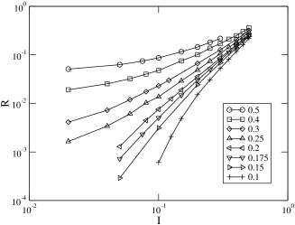
Figure 1: Log-log plots of $I-R$ curves at various temperatures.

First, we study the possible glass phase transition. The glass transition temperature was estimated to be $T_{g}\approx 0.20$ by several groupsRSJ ; Choi ; chen . So the current-voltage characteristics are measured at various temperatures ranging from $0.1$ to $0.5$, which cover the previous $T_{g}$. At each temperature, we try to probe the system at currents as low as possible. Fig.1 displays the resistivity $R=V/I$ as a function of current $I$ at various temperatures in a log-log scale. It is obvious that, at lower temperatures, $R$ tends to zero as the current decreases, suggesting that there is a true superconducting phase with zero linear resistivity. While at higher temperatures, $R$ tends to a finite value, corresponding to Ohmic resistivity in the vortex liquid. These observations reveal strong evidence of the existence of the low-temperature glass phase in the 2D gauge glass model.

Assuming that the VG transition is continuous and characterized by the divergence of the characteristic length and time scales $t\sim\xi^{z}$ ( $z$ is the dynamic exponent), Fisher, Fisher, and Huse FFH proposed the following dynamic scaling ansatz to analyze the glass transition from a vortex liquid with Ohmic resistivity to a superconducting glass state

$$TR\xi^{z+2-d}=\Psi_{\pm}(I\xi^{d-1}/T),$$ (4)

where $d$ is the dimension of the system ($d=2$ in this paper), $\xi\propto\mid T/T_{g}-1\mid^{-\nu}$ is the correlation length which diverges at the transition and $\Psi_{\pm}(x)$ are scaling functions for $T>T_{g}$ and $T<T_{g}$, respectively. Eq.(4) is often used to scale the measured current-voltage data in the VG transitions in experiments.

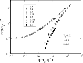
Figure 2: Dynamic scaling of $I-R$ data at various temperatures according to Eq. (4).

To extract the critical behavior from the numerical results of the current-voltage characteristics, we also perform a dynamic scaling analysis. As shown in Fig.2, with $T_{g}=0.22\pm 0.02$ , $z=2.0\pm 0.1$, and $\nu=1.8\pm 0.1$, an excellent collapse is achieved according to Eq.(4) except for the curve of $T=0.1$. The errors are estimated by tuning these critical values until the collapses become poor evidently. The curve at $T=0.1$ is obviously beyond the critical regime.

The finite-size effects are particularly significant at temperatures sufficiently close to $T_{g}$ when the correlation length exceeds the system size. For the temperatures considered here and the very large system size $L=128$, we believe that the finite-size effects are negligible in the present simulations. To confirm this point, we perform particular simulations right at $T_{g}=0.22$ obtained above for different system sizes. At $T_{g}$, the correlation length is cut off by the system size in any finite system, so the scaling form Eq.(4) becomes

$$T_{g}RL^{z}=\Psi(IL/T_{g}).$$ (5)

A good collapse is illustrated in Fig.3 with $z=2.0$. This consistency demonstrates that the results estimated from Fig.2 are reliable. Therefore new evidence of a finite-temperature glass transition is provided convincingly in the 2D gauge glass model.

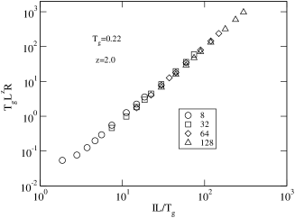
Figure 3: Dynamic scaling of $I-R$ data at $T_{g}=0.22$ according to Eq.(5).

The obtained $T_{g}$ and dynamic exponent $z$ are well consistent with those in equilibrium RSJ simulationsRSJ and Monte Carlo simulationsChoi . The value of $\nu$ estimated here is larger than those ( $1.1\sim 1.2$) obtained in several simulationsChoi ; RSJ , but still falls in the range of $1.0\sim 2.0$ usually observed at the VG transitions experimentally. Within the same RSJ dynamics, the finite-size scaling for the linear resistivity for sample sizes $L\leq 10$ gives $\nu=1.2(2)$ in Ref.RSJ . The discrepancy may originate from the different scaling method and sizes used. In a previous conference paper chen by one of the present author and collaborators, with the uses of a different simulation approach and a scaling form different from Eq. (4) slightly by removing temperature $T$, $T_{g}=0.22$ , $z=2.0$, and $\nu=1.2$ were obtained. The present simulation gives larger value of $\nu$.

Based on the analysis of data at temperatures above $T_{g}=0.22$, previous RSJ simulationsHyman ; granato with an open boundary condition in the 2D gauge glass model demonstrated a zero-temperature criticality. It has been shown that the voltage drop next to the boundary regime is particularly large and dominates the total voltage drop across the sample at low currentskim ; simkin ; Choi1 . Therefore, one should measure the voltage drop inside the sampleChoi1 ; chen1 . So the conclusion based on the total voltage drop across the system with the open boundary conditionHyman ; granato may not be reliable.

Interestingly, in experiments on Nb wire networksLiang , the critical exponents $\nu=1.7\sim 1.9$ were obtained for high filling factors $f=1/2,0.618$, and $2/5$, which are very close to the present value. It was suggested in Ref. Yun that the superconducting state and transitions in the networks become independent of $f$ in the gauge glass limit. The further work is needed to clarify the relation between the experimental observations and the present simulations.

To shed some light on the nature of this low-temperature glass phase, we will study the depinning and creep phenomena.

At zero temperature, we start from high currents with random initial phase configurations. The currents are then lowered step by step. The steady-state phase configurations obtained at higher currents are chosen to be the initial phase configurations of lower currents in the next step. It becomes more and more difficult to measure the voltage with decreasing currents. In the vicinity of the critical current, a huge amount of computer time is consumed to get accurate results. Fig.4 presents the current-voltage characteristics at $T=0$ in a log-log scale. We observe a continuous depinning transition with a unique depinning currentFisher , which can be described as $V\propto(I-I_{c})^{\beta}$ with $I_{c}=0.2165\pm 0.0005$ and $\beta=1.892\pm 0.003$. Note that the depinning exponent $\beta$ is greater than $1$, consistent with the mean field studies of charge density wave modelsFisher .

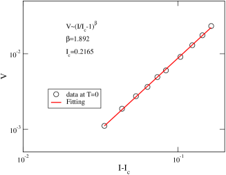
Figure 4: Log-log plot of $V$ versus $(I-I_{c})$ curve at zero temperature.

At low temperatures, the current-voltage characteristics are rounded near the zero-temperature critical current due to thermal fluctuations. An obvious crossover between the depinning and creep motion can be observed around $I_{c}$ at lower accessible temperatures. In order to address the thermal rounding of the depinning transition, FisherFisher first suggested to map this system to ferromagnets in fields where the second-order phase transitions occur. This mapping was later extended to the random-field Ising modelRoters and flux lines in type-II superconductorsluo . If the voltage is identified as the order parameter, the current and temperature are equivalent to the inverse temperature and the field in ferromagnetic systems, respectively, analogous to the second-order phase transitions, a scaling relation among the voltage, current and temperature in the present model should follow the form

$$~{}V(T,I)=T^{1/\delta}S[T^{-1/\beta\delta}(1-I_{c}/I)],$$ (6)

where $S(x)$ is a scaling function with $S(x\rightarrow 0)=$const.

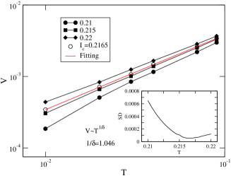
Figure 5: Log-log plots of $V-T$ curves at three currents around $I_{c}$.

It is implied in Eq.(6) that right at $I=I_{c}$ the voltage shows a power-law behavior $V(T,I=I_{c})\propto T^{1/\delta}$, providing a tool to determine the critical exponent $1/\delta$. The log-log $V-T$ curves are plotted in Fig. 5 at three currents around $I_{c}$. We can see that the critical current is between $0.21$ and $0.22$. The values of voltage at other currents within $(0.21,0.22)$ can be evaluated by quadratic interpolation. The square deviations from the power law can be calculated. The current at which the square deviation is minimum can be considered as the critical current $I_{c}=0.2165\pm 0.0005$, consistent with that obtained at zero temperature. The temperature dependence of voltage at the critical current is also exhibited in Fig.5, yielding $1/\delta=1.046\pm 0.002$.

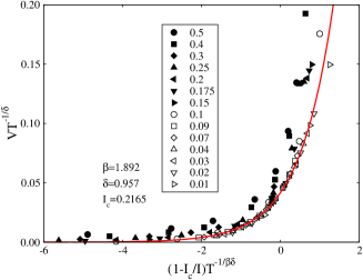
Figure 6: Scaling plot of $I-V$ data at various temperatures according to Eq.(6).

With the values of $\beta$, $\delta$ and $I_{c}$ obtained above, according to the scaling relation Eq.(6), a scaling plot of the simulated current-voltage data in a wide range of temperature is presented in Fig.6 without any adjustable parameter. A perfect collapse of the data for temperatures $T\leq 0.10$, far below $T_{g}=0.22$, to a single curve for currents less than $I_{c}$ is clearly shown. This collapse can be fitted well to an exponential function $y=0.0417$exp$(1.17x)$, which is also plotted in the Fig.6 with a solid line. Note that the product of the two exponents $\beta\delta$ describes the temperature dependence of the creep law. Interestingly, $\beta\delta\approx 1.81$ deviates from unity, demonstrating that the creep law is a non-Arrhenius type. At higher temperatures, say $T>0.1$, deviations from the scaling relation are also observed in Fig.6, which can be attributed to strong thermal fluctuations. The non-Arrhenius type creep phenomena only take place at low temperatures.

IV Summary

We have performed large-scale dynamic simulations of the 2D gauge glass model within the RSJ dynamics. The strong evidence of the low-temperature glass phase is provided in the dynamic sense. By the dynamic scaling analysis, two perfect collapses of simulated current-voltage data are achieved with $T_{g}=0.22\pm 0.02$ , $z=2.0\pm 0.1$, and $\nu=1.8\pm 0.1$. The values of $T_{g}$ and $z$ are in agreement with those in the previous equilibrium Monte Carlo simulations. While the value of $\nu$ is larger than that in literature, which is, however, closer to that in experiments in the gauge glass limit. We have also studied the depinning transition at zero temperature and creep motion at low temperatures in detail. A genuine continuous depinning transition is observed at zero temperature. With the notion of scaling and the critical exponents obtained from the simulations at zero temperature and at the critical current, a perfect collapse of the current-voltage data at low temperatures is exhibited. The value of $\beta\delta$ deviates from unity and the scaling curve is fitted well by an exponential function, suggesting a non-Arrhenius type creep motion in the glass phase of the 2D gauge glass model.

It is worthy to note that in this model the current-voltage characteristics in the whole temperature regime below $T_{g}$ can almost be described in the framework of two critical phenomena. One is the thermal rounding of the depinning transition, which is a second-order-like phase transition. The other is the celebrated VG transition. Further experimental and theoretical studies are needed to clarify the relation between the present observations and experimental findings.

V Acknowledgements

We acknowledge useful discussions with X. Hu and M. B. Luo. This work was supported by National Natural Science Foundation of China under Grant No. 10574107 and 10774128, PNCET and PCSIRT in University in China, National Basic Research Program of China (Grant No. 2006CB601003).

References

- (1) R. H. Koch, V. Foglietti, W. J. Gallagher, G. Koren, A. Gupta, and M. P. A. Fisher, Phys. Rev. Lett. 63, 1511 (1989); R. H. Koch, V. Foglietti, and M. P. A. Fisher, Phys. Rev. Lett. 64, 2586 (1990); P. Gammel, L. Schneemeyer, and D. Bishop, Phys. Rev. Lett. 66, 953 (1991); T. Klein, A. Conde-Gallardo, J. Marcus, and C. Escribe-Filippini, P. Samuely, P. Szabó, and A. G. M. Jansen, Phys. Rev. B 58, 12411(1998); A. M. Petrean, L. M. Paulius, W.-K. Kwok, J. A. Fendrich, and G. W. Crabtree, Phys. Rev. Lett. 84, 5852 (2000); U. Divakar, A. J. Drew, S. L. Lee, R. Gilardi, J. Mesot, F. Y. Ogrin, D. Charalambous, E. M. Forgan, G. I. Menon, N. Momono, M. Oda, C. D. Dewhurst, and C. Baines, Phys. Rev. Lett. 92, 237004 (2004); J. E. Villegas and J. L. Vicent, Phys. Rev. B 71, 144522(2005).
- (2) D. A. Huse and H. S. Seung, Phys. Rev. B 42, R1059 (1990).
- (3) H. G. Katzgraber, D. Würtz, and G. Blatter, Phys. Rev. B 75 214511 (2007).
- (4) A. Vestergren, J. Lidmar, and M. Wallin, Phys. Rev. Lett. 88, 117004 (2002).
- (5) P. Olsson, Phys. Rev. Lett. 91, 077002 (2003); H. Kawamura, Phys. Rev. B 68, 220502(R) (2003).
- (6) J. Lidmar, Phys. Rev. Lett. 91, 097001(2003); Rodriguez, Phys. Rev. B 69, 100503 (R) (2004).
- (7) J. M. Kosterlitz and N. Akino, Phys. Rev. Lett. 81, 4672 (1998); T. Olson and A. P. Young, Phys. Rev. B 61, 12467(2000); H. G. Katzgraber and I. A. Campbell, Phys. Rev. B 69, 094413 (2004).
- (8) C. Dekker, P. J. M. Wöltgens, R. H. Koch, B. W. Hussey, and A. Gupta, Phys. Rev. Lett. 69, 2717 (1992).
- (9) A. Sawa, H. Yamasaki, Y. Mawatari, H. Obara, M. Umeda, and S. Kosaka, Phys. Rev. B 58, 2868 (1998).
- (10) Y. J. Yun, I. C. Baek, M. Y. Choi, Europhys. Lett. 76, 271 (2006).
- (11) M. P. A. Fisher, T. A. Tokuyasu, and A. P. Young, Phys. Rev. Lett. 66, 2931 (1991); J. D. Reger and A. P. Young, J. Phys. A 26, L1067 (1993); H. Nishimori, Physica A 205, 1(1994); H. G. Katzgraber, Phys. Rev. B 67, 180402(R) (2003); M. Nikolaou and M. Wallin, Phys. Rev. B 69, 184512 (2004).
- (12) M. J. P. Gingras, Phys. Rev. B 45, 7547 (1992); J. M. Kosterlitz and M. V. Simkin, Phys. Rev. Lett. 79, 1098 (1997); N. Akino and J. M. Kosterlitz, Phys. Rev. B 66, 054536 (2002).
- (13) L. H. Tang and P. Q. Tong, Phys. Rev. Lett. 94,207204 (2005).
- (14) R. A. Hyman, M. Wallin, M. P. A. Fisher, S. M. Girvin, A. P. Young, Phys. Rev. B 51, 15304(1995)
- (15) E. Granato, Phys. Rev. B 58,11161(1998).
- (16) Y. H. Li, Phys. Rev. Lett. 69, 1819(1992).
- (17) B. J. Kim, Phys. Rev. B 62, 644 (2000).
- (18) Q. H. Chen, A. Tanaka and X. Hu, Physica B329-333, 1413(2003).
- (19) J. Um, B. J. Kim, P. Minnhagen, M. Y. Choi, and S.-I. Lee, Phys. Rev. B 74, 094516 (2006).
- (20) M. Y. Choi and S. Y. Park, Phys. Rev. B 60, 4070 (1999); P. Holme, B. J. Kim, and P. Minnhagen, Phys. Rev. B 67, 104510 (2003);
- (21) T. Nattermann, Phys. Rev. Lett. 64, 2454(1990).
- (22) P. Chauve, T. Giamarchi, and P.L.Doussal, Phys. Rev. B 62, 6241(2000).
- (23) M. Müller , D. A. Gorokhov, and G. Blatter, Phys. Rev. B 63 , 184305(2001).
- (24) L. Roters, A. Hucht, S. Lübeck, U. Nowak and K. D. Usadel, Phys. Rev. E 60, 5202(1999).
- (25) M. B. Luo and X. Hu, Phys. Rev. Lett. 98, 267002(2007).
- (26) P. Olsson, Phys. Rev. Lett. 98, 097001(2007).
- (27) B. J. Kim, P. Minnhagen and P. Olsson, Phys. Rev. B 59, 11506 (1999).
- (28) Q. H. Chen, L. H. Tang, and P. Q. Tong, Phys. Rev. Lett. 87, 067001(2001); L. H. Tang and Q. H. Chen, Phys. Rev. B 67, 024508 (2003).
- (29) Q. H. Chen and X. Hu, Phys. Rev. Lett. 90, 117005(2003); Q. H. Chen and X. Hu, Phys. Rev. B 75, 064504 (2007).
- (30) D. Fisher, M. P. A. Fisher, and D. Huse, Phys. Rev. B 43, 130 (1991).
- (31) M. V. Simkin and J. M. Kosterlitz, Phys. Rev. B 55, 11646 (1997)
- (32) M. Y. Choi, G. S. Jeon, and M. Yoon, Phys. Rev. B 62, 5357 (2000).
- (33) X. S. Ling, H. J. Lezec, M. J. Higgins, J. S. Tsai, J. Fujita, H. Numata, Y. Nakamura, Y. Ochiai, Chao Tang, P. M. Chaikin, and S. Bhattacharya, Phys. Rev. Lett. 76, 2989(1996)
- (34) D. S. Fisher, Phys. Rev. Lett. 50, 1486 (1983); Phys. Rev. B 31, 1396 (1985).