Self tuning phase separation in a model with competing interactions inspired by biological cell polarization

Abstract

We present a theoretical study of a system with competing short-range ferromagnetic attraction and a long-range anti-ferromagnetic repulsion, in the presence of a uniform external magnetic field. The interplay between these interactions, at sufficiently low temperature, leads to the self-tuning of the magnetization to a value which triggers phase coexistence, even in the presence of the external field. The investigation of this phenomenon is performed using a Ginzburg-Landau functional in the limit of an infinite number of order parameter components (large $N$ model). The scalar version of the model is expected to describe the phase separation taking place on a cell surface when this is immersed in a uniform concentration of chemical stimulant. A phase diagram is obtained as function of the external field and the intensity of the long-range repulsion. The time evolution of order parameter and of the structure factor in a relaxation process are studied in different regions of the phase diagram.

I Introduction

Several natural and social processes are governed by competing interactions. Often the interplay between opposite actions produces ordered phases and symmetry breaking events. For example, models based on competing interactions are able to explain lamellar phases in charged colloids TCpre2007 , pattern formation in magnetic films, Languimir monolayers and liquid crystals Giuliani and some market behaviors econofis . In living organisms there is an important example of these processes: the spatial orientation of eukaryotic cells alberts called eukaryotic directional sensing. Many eukaryotic cells are able to orient (polarize) for moving along directions after an external stimulation. This process is fundamental for important biological functions like morphogenesis of organs and tissues, wound healing, immune response, social behaviors of some amoeboid cells. The process of orientation takes place on the cell membrane where the pattern formation of domains of two different enzymes determines a symmetry breaking which triggers the directional sensing JMD+04 . Pattern formation occurs as a response to an external stimulation, usually a chemical signal activating specific receptors on the cell surface, enhanced by a cascade of chemical reactions leading to the cell polarization (see Ref. GCT+05 and references therein). Experimental observations PRG+04 suggest that the domain formation is a consequence of self-organization of molecular patches.

Let us briefly summarize the biological mechanism of directional sensing. It can be explained in term of the interplay between two enzymes: PTEN (phosphatase and tesin homolog) and PI3K (phosphatidylinotisol 3-kinase). This interplay is mediated by two lipids: the PIP₂ (phosphatidylinotisol bisphosphate) and the PIP₃ (phosphatidylinotisol trisphosphate). Before stimulation, the cell membrane is populated only by the PTEN enzyme with its product PIP₂ but, when the external chemoattractant is switched on, the enzyme PI3K goes from cytoplasm to the cell membrane and binds to receptors. Then, the interplay between the two enzymes takes place: the PI3K catalyzes PIP₂ in PIP₃ and PTEN catalyzes PIP₃ in PIP₂. The enzymes can bind to the respective lipid products which diffuse over the membrane. Enzymes can unbind from membrane and quickly diffuse in cytoplasm binding again in another place of the membrane. Catalysis and lipides diffusion mediate an effective short-range attraction between enzymes of the same type. The quick diffusion of enzymes in the cytoplasm mediates a long range interaction. The combination of these actions produces the phase separation of a PI3K rich zone and a PTEN rich zone.

The natural framework to treat the process, from a physical point of view, is the statistical physics of phase separation, which is useful to understand and describe in synthetic way the behavior of many complex systems that give rise to organization and pattern formation Domb ; preSagDes1994 . The spatial organization phenomena described above have the characteristic of self-organized phase separation processes, where the cell state, driven by an external field, decays into the coexistence of two chemical phases, spatially localized in different regions. It was shown recently, by Monte Carlo simulation in a lattice gas model epl+FDGC+08 , that the phenomenology of directional sensing can be obtained by using an effective free energy. A similar point of view was used in the recent papers of Gamba et al. GKL+07 ; GKLO+08 . The remarkable physical characteristic of the process is that the orientation is possible for a wide range of external chemical attractant Zig77 . Namely, the phase coexistence and separation is possible for different values of an external field. In the lattice gas model epl+FDGC+08 , a long range repulsion, derived from the interaction with a finite cytosolic reservoir of total enzymes and the interaction with an external field, modelling the action of the chemical attractant, give rise to coexistence for an interval of values of the external field. A short-range attraction between enzymes, derived from their catalytic actions on lipids and diffusion, gives rise to a coarsening process which produces phase separation. A similar mechanism operates in some econophysics models econofis based on two major conflicting interactions in economy, the tendency of a trader to follow the actions of his neighbors and the tendency to follow the actions of the minority. In the language of magnetic systems, which we will use throughout this paper, the first tendency can be modelled by a short-range ferromagnetic interaction, while the second one by an antiferromagnetic long range interaction.

Inspired by the mechanism of eukaryotic directional sensing and motivated by its wide applicability, here we present the analytical treatment of a system with competing short-range attraction and long-range repulsion, under the action of a uniform external field. This is done in the framework of the time dependent Ginzburg-Landau (TDGL) theory for the evolution of the order parameter. The analytical tractability of the dynamics is achieved considering a vector order parameter in the limit of an infinite number of components (large $N$ limit) preCRZ1994 . The equations of motion are derived in the scheme of non conserved order parameter, corresponding to the absence of local concentration of enzymes.

The large $N$ limit is a powerful method to obtain analytical results, nevertheless it is necessary to keep in mind some important differences with the nonlinear models usually employed in the description of phase ordering when the order parameter is a scalar, such as kinetic Ising models or the TDGL with $\phi^{4}$ interaction Bra95 . The basic difference is in the mechanism of equilibration after a symmetric quench below the critical point. In the nonlinear models the system responds to the dynamical instability by the formation and growth, through coarsening, of domains of the ordered phases. This leads to the development of a bimodal probability distribution for the local magnetization, which eventually ought to evolve into the symmetric mixture of the two possible broken symmetry ordered phases footnote . This we call an ordering process. In the large $N$ limit, instead, the development of a bimodal distribution, and therefore ordering, is not possible, since, as it will be clear below, the system is effectively linearized and the statistics are Gaussian. Then, the response to the dynamical instability takes place through the development of macroscopic fluctuations in the most unstable Fourier component of the order parameter, through a process which is formally identical to the one leading to the formation of the condensate in the low temperature phase of the ideal Bose gas. We refer to this equilibration mechanism as condensation of fluctuations. The differences between the two equilibration processes have been investigated in detail in Ref. CCZ ; Fusco .

The remarkable feature of the large $N$ limit, and the reason for its wide use, is that despite the considerable difference in the physical processes of equilibration, the phenomenology of the observables of interest, such as correlation functions and response functions, is the same as in the nonlinear models, apart for obvious quantitative discrepancies, like the values of exponents or the shape of scaling functions. The typical example is that of the equal time structure factor, which displays dynamical scaling and the growth of the Bragg peak in the large $N$ limit CZ , exactly as in the nonlinear models. It is, then, matter of interpretation in one case to read the growth of the Bragg peak as revealing domain coarsening and, in the other, condensation of fluctuations. There is, by now, a vast body of literature documenting the robustness of the large $N$ limit in reproducing the phenomenology of phase ordering in a large variety of models, warranting to overlook the distinction between ordering and condensation, as we shall do in this paper, when one is interested in the main qualitative features of the process.

The paper is organized as follows. In section II we carry out the large $N$ limit on the TDGL model for a vector order parameter, deriving the basic equations. In section III we study the equilibrium properties of the system, obtaining the phase diagram in the temperature and external field plane, parameterized by the strength of the long-range repulsion. This delimits the region of parameters where condensation or, equivalently, phase coexistence and separation are possible. Section IV is devoted to the study the time behavior of the average value of the order parameter (magnetization) and of the correlation function. We recall that in the scalar case the magnetization represents the concentration difference between the two species of enzymes. Concluding remarks are presented in section V.

II The model

The system is modelled by a free energy functional of the form

$${\cal H}[\vec{\phi}] = \int_{V}d\vec{x}\left\{{1\over 2}(\nabla\vec{\phi})^{2}+{r\over 2}(\vec{\phi}\cdot\vec{\phi})+{g\over 4N}(\vec{\phi}\cdot\vec{\phi})^{2}-\vec{H}(\vec{x})\cdot\vec{\phi}(\vec{x})\right\}$$ (1)

$$+ {1\over 2}{\lambda\over V}\left[\int_{V}d\vec{x}\,\vec{\phi}\right]^{2}$$

where $\vec{\phi}=(\phi_{1},...,\phi_{N})$ is an $N$ component vector order parameter. We shall take $r<0,\,g>0,\,H\sim{\cal O}(N^{1/2})$, $V$ is the volume of the system and $\lambda>0$ is an antiferromagnetic coupling. We shall consider the static and dynamic properties of the model.

As is well known from the theory of critical phenomena, the introduction of an $N$ component order parameter is a very convenient technical device to generate controlled and systematic correction about mean field behavior, using $1/N$ as an expansion parameter ZJ . We shall limit the treatment to the lowest (mean field) order by taking the large $N$ limit ($N\rightarrow\infty$).

II.1 Equation of motion

In the framework of TDGL model for the dynamics

$${\partial\vec{\phi}(\vec{x},t)\over\partial t}=-{\delta{\cal H}[\vec{\phi}]\over\delta\vec{\phi}}(\vec{x},t)+\vec{\eta}(\vec{x},t)$$ (2)

where $\vec{\eta}(\vec{x},t)$ is the white noise at temperature $T$, with zero average and correlator

$$\langle\eta_{\alpha}(\vec{x},t)\eta_{\beta}(\vec{x}^{\prime},t^{\prime})\rangle=2T\delta_{\alpha\beta}\delta(\vec{x}-\vec{x}^{\prime})\delta(t-t^{\prime})$$

the equation of motion of the order parameter is given by

$${\partial\vec{\phi}(\vec{x},t)\over\partial t} = -\left[-\nabla^{2}\vec{\phi}(\vec{x},t)+r\,\vec{\phi}(\vec{x},t)+{g\over N}(\vec{\phi}\cdot\vec{\phi})\vec{\phi}(\vec{x},t)-\vec{H}(\vec{x})\right]$$ (3)

$$- {\lambda\over V}\int_{V}d\vec{x}\,\vec{\phi}(\vec{x},t)+\vec{\eta}(\vec{x},t).$$

Since the external field breaks the rotational symmetry in the order parameter space, it is convenient to introduce the longitudinal and transverse components with respect $\vec{H}(\vec{x})$

$$\vec{\phi}=\vec{\phi}_{\parallel}+\vec{\phi}_{\perp}$$ (4)

and then to split the longitudinal component into the sum

$$\vec{\phi}_{\parallel}(\vec{x},t)=\vec{M}(\vec{x},t)+\vec{\psi}(\vec{x},t)$$ (5)

where $\vec{M}(\vec{x},t)=\langle\vec{\phi}_{\parallel}(\vec{x},t)\rangle$ is the magnetization, while the average longitudinal fluctuations vanish $\langle\vec{\psi}(\vec{x},t)\rangle\equiv 0$ by construction. The angular brackets denote the average over both the initial condition and the thermal noise. In the following we shall take a reference frame with the $1$-axis along the longitudinal direction.

Assuming, next, $M\sim{\cal O}(N^{1/2})$, $\psi\sim{\cal O}(1)$ and comparing terms of the same order of magnitude in $N$, to leading order we get the pair of equations

$${\partial m\over\partial t}=-\left[-\nabla^{2}+r+gm^{2}+gS\right]m+\big{(}h-{\lambda\over V}\int_{V}d\vec{x}\,m\big{)}$$ (6)

and

$${\partial\vec{\phi}_{\perp}\over\partial t}=-\left[\Big{(}-\nabla^{2}+r+gm^{2}+gS\Big{)}\vec{\phi}_{\perp}+{\lambda\over V}\int_{V}d\vec{x}\,\vec{\phi}_{\perp}\right]+\vec{\eta}_{\perp}$$ (7)

where $m\equiv m(x,t)$ and $h\equiv h(x,t)$ are the following rescaled quantities

$$m(\vec{x},t)=M(\vec{x},t)/N^{1/2},\;\;h(\vec{x},t)=H(\vec{x},t)/N^{1/2}.$$ (8)

In the large $N$ limit the quantity $S(\vec{x},t)$ is given by the self-averaged fluctuations

$$\lim_{N\to\infty}{1\over N}(\vec{\phi}_{\perp}\cdot\vec{\phi}_{\perp})=\langle\phi_{\alpha}\phi_{\alpha}\rangle=S(\vec{x},t)$$ (9)

of the generic transverse component $\phi_{\alpha}$. Furthermore, since in Eq. (7) the components of $\vec{\phi}_{\perp}$ are effectively decoupled, from now on we shall refer to the equation for the generic component omitting the $\alpha$ subscript.

Taking a space and time independent external field $h$ and space translation invariant initial conditions, we can assume space translation invariance to hold at all times. Hence, Fourier transforming with respect to space, and introducing the equal-time transverse structure factor

$$\langle\phi(\vec{k},t)\phi(\vec{k}^{\prime},t)\rangle=C_{\perp}(\vec{k},t)V\delta_{\vec{k}+\vec{k}^{\prime},0}$$ (10)

we obtain the closed set of equations

$${\partial m(t)\over\partial t}=-\omega(0,t)m(t)+h$$ (11)

$${\partial C_{\perp}(\vec{k},t)\over\partial t}=-2\omega(k,t)C_{\perp}(\vec{k},t)+2T$$ (12)

$$S(t)={1\over V}\sum_{\vec{k}}C_{\perp}(\vec{k},t)$$ (13)

with $m(t)\equiv m(\vec{k}=0,t)$ and $\omega(k,t)$ defined by

$$\omega(k,t)=k^{2}+\lambda\delta_{k,0}+r+g(m^{2}+S)$$ (14)

and the noise correlator in Fourier space given by

$$\langle\eta(\vec{k},t)\eta(\vec{k}^{\prime},t^{\prime})\rangle=2TV\delta_{\vec{k}+\vec{k}^{\prime},0}\delta(t-t^{\prime}).$$

With periodic boundary conditions the wave vector runs over $\vec{k}={2\pi\over L}\vec{n}$, where $\vec{n}$ is a vector with integer components and $L^{d}=V$. Furthermore, sums over $\vec{k}$ like the one in Eq. (13) are cutoff to the upper value $k_{max}=\Lambda$, where $\Lambda^{-1}$ is related to a characteristic microscopic length, for instance the lattice spacing of an underlying lattice. Finally, the longitudinal fluctuations $\psi$ have been dropped since do not give any contribution to leading order.

III Static properties and phase diagram

If equilibrium is reached, all quantities become time independent. Rewriting Eq. (14) as

$$\omega(k)=\left\{\begin{array}[]{ll}\lambda+\mu,\qquad$for$\qquad k=0\\ k^{2}+\mu,\qquad$for$\qquad k\neq 0\end{array}\right.$$ (15)

with

$$\mu=r+g(m^{2}+S)$$ (16)

and putting to zero the time derivatives, from Eqs. (11), (12) and (13) we obtain the set of equations

$$(\lambda+\mu)m=h$$ (17)

$$\omega(k)C_{\perp}(\vec{k})=T$$ (18)

$$S={1\over V}\sum_{\vec{k}}C_{\perp}(\vec{k}).$$ (19)

From Eqs. (10) and (18) follows $C_{\perp}(\vec{k})\geq 0$ and $\omega(k)\geq 0$, respectively. The latter inequality, because of Eq. (15), requires

$$\mu\geq\mu_{min}=-k^{2}_{min}$$ (20)

where $k_{min}\sim 1/L$ is the minimum allowed value of $k\neq 0$. Therefore, for a given $\lambda$ and for $V$ sufficiently large, $\lambda+\mu>0$ and Eq. (17) can be rewritten as

$$m={h\over\lambda+\mu}.$$ (21)

In the same way, from Eq. (18) we can write

$$C_{\perp}(\vec{k})=\left\{\begin{array}[]{ll}T/(\lambda+\mu),\qquad$for$\qquad k=0\\ T/(k^{2}+\mu),\qquad$for$\qquad k\geq k_{min}\end{array}\right.$$ (22)

where $C_{\perp}(\vec{k}_{min})$ diverges as $\mu$ approaches $\mu_{min}$. Notice that $\mu$ can be identified with the inverse square transverse correlation length $\xi^{-2}$.

In order to obtain the full solution, we must now determine how $\mu$ depends on the parameters of the problem $(T,h,V,\lambda)$. In principle, this can be done by inserting the above results into Eq. (16) and solving the basic self-consistency equation

$$\mu-g\left({h\over\lambda+\mu}\right)^{2}=r+{g\over V}{T\over\lambda+\mu}+{Tg\over V}\sum_{\vec{k}\neq 0}{1\over k^{2}+\mu}.$$ (23)

However, for our purposes general considerations are sufficient, without actually solving the above equation. For $V$ sufficiently large the second term in the right hand side can be neglected and the equation can be rewritten in the form

$$\mu-g\left({h\over\lambda+\mu}\right)^{2}=r+{g\over V}{T\over\mu-\mu_{min}}+{Tg\over V}\sum_{\vec{k}>\vec{k}_{min}}{1\over k^{2}+\mu}$$ (24)

where the $k_{min}$ term has been extracted from underneath the sum. Letting $\mu$ to vary from $\mu_{min}$ to $\infty$, the left hand side is a monotonously increasing function of $\mu$, while the right hand side diverges at $\mu_{min}$ and decreases monotonously with increasing $\mu$. Therefore, for any finite $V$, there exists a solution $\mu^{*}(V)>\mu_{min}$. Looking at Eqs. (21) and (22), this means that the system behaves paramagnetic all over the $(T,h)$ plane, with a finite structure factor. The difference with respect to what one would have in the purely short-range model, due to $\lambda\neq 0$, is revealed by the anomaly (22) in the structure factor at $k=0$ and by the reduction of the magnetization in Eq. (21). Rewriting the latter as $\mu^{*}(V)m=h_{eff}$ with

$$h_{eff}=h-\lambda m,$$ (25)

we see that the reduction of the magnetization comes about through a feedback mechanism, whereby the external field $h$, via the long-range interaction, is substituted by $h_{eff}$.

Let us now see what happens in the infinite volume limit. From Eq. (20) follows $\mu_{min}\rightarrow 0^{-}$ and there are two possibilities

$$\lim_{V\to\infty}\mu^{*}(V)=\left\{\begin{array}[]{ll}\mu^{*}>0\\ \mu^{*}=0.\end{array}\right.$$ (26)

In the first case, the second term in the right hand side of Eq. (24) can be neglected yielding

$$\mu-g\left({h\over\lambda+\mu}\right)^{2}=r+TgB(\mu)$$ (27)

where

$$B(\mu)=\lim_{V\to\infty}{1\over V}\sum_{\vec{k}\neq 0}{1\over k^{2}+\mu}=K_{d}\int_{0}^{\Lambda}dk\,{k^{d-1}\over k^{2}+\mu}$$ (28)

is a monotonously decreasing function of $\mu$ with the maximum value

$$B(0)=\left\{\begin{array}[]{ll}K_{d}{\Lambda^{d-2}\over d-2},\qquad$for$\qquad d>2\\ $divergent for$\qquad d\leq 2\end{array}\right.$$ (29)

with $K_{d}=[2^{d-1}\pi^{d/2}\Gamma(d/2)]^{-1}$ being the $d$-dimensional solid angle nota1 and $\Gamma(d/2)$ the Euler gamma function. Hence, Eq. (27) admits a positive solution if $T$ is greater than the $h$-dependent critical temperature

$$T_{C}(h)=-{r+gh^{2}/\lambda^{2}\over gB(0)}$$ (30)

which vanishes for $d\leq 2$ and for any $h$, while it is finite for $d>2$ reaching the maximum value $T_{C}(0)=-r/gB(0)$ for $h=0$ and decreasing to zero when $h$ reaches the limit values $\pm h_{C}$ (see Fig. 1) with

$$h_{C}=\lambda(-r/g)^{1/2}.$$ (31)

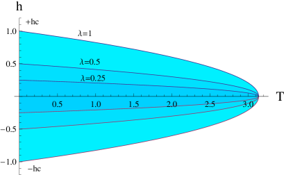
Figure 1: (Color online) Phase diagram showing the $\lambda$ dependence of the region within which condensation of the transverse fluctuation takes place. The presence of a condensate, in the blue regions, corresponds to phase separation and coexistence in the corresponding scalar model. In this and in all the other figures $g=-r=1$, $\Lambda=2\pi$ and $d=3$, yielding $T_{C}(0)=\pi$.

Conversely, if $T$ and $h$ are such that $T<T_{C}(h)$, Eq. (27) cannot be satisfied. This means that the second of the two possibilities in Eq. (26) applies, requiring to keep also the second term in the right hand side of Eq. (24), which we rewrite as

$$\mu-g\left({h\over\lambda+\mu}\right)^{2}=r+{g\over V}C_{\perp}(\vec{k}_{min})+TgB(\mu).$$ (32)

Since this is satisfied for $\mu=0$, we get

$$C_{\perp}(\vec{k}_{min})=V\left[-{r\over g}-\left({h\over\lambda}\right)^{2}\right]\left[{T_{C}(h)-T\over T_{C}(h)}\right]$$ (33)

showing that $C_{\perp}(\vec{k}_{min})$, for $T<T_{C}(h)$, diverges like the volume in order to give a finite contribution in the right hand side of Eq. (32).

Summarizing, in the infinite volume limit

$$m=\left\{\begin{array}[]{ll}h/(\lambda+\mu^{*}),\qquad$for$\qquad T>T_{C}(h)\\ h/\lambda,\qquad$for$\qquad T<T_{C}(h)\end{array}\right.$$ (34)

where $\mu^{*}>0$, and

$$C_{\perp}(\vec{k})=\left\{\begin{array}[]{ll}T/(k^{2}+\mu^{*}),\qquad$for$\qquad T>T_{C}(h)\\ T/k^{2}+{\cal M}^{2}(T)\delta(\vec{k}-0^{+}),\qquad$for$\qquad T<T_{C}(h)\end{array}\right.$$ (35)

showing that there is condensation of transverse fluctuation at $k=0^{+}$ for $T<T_{C}(h)$, with the size of the condensate given by

$${\cal M}^{2}(T)=\left[-{r\over g}-\left({h\over\lambda}\right)^{2}\right]\left[{T_{C}(h)-T\over T_{C}(h)}\right].$$ (36)

In order to understand this result, it should be recalled that in the purely short-range large $N$ model the phase transition occurs only on the $h=0$ axis, where for $T<T_{C}(0)$ the condensation of fluctuations takes place CCZ at $k=0$. Condensation of fluctuations means that $C_{\perp}(\vec{k}=0)$ becomes macroscopic in order to equilibrate the system below $T_{C}(0)$ without breaking the symmetry, through a mechanism very similar to that of the Bose-Einstein condensation, as mentioned in the Introduction. No other mechanism is available, since the large $N$ limit renders the system effectively Gaussian CCZ ; Fusco . However, condensation of fluctuations produces the onset of a Bragg peak at $\vec{k}=0$ and, therefore, a phenomenology of the structure factor which is indistinguishable from that due to the occurrence of phase separation in the nonlinear models Bra95 . When $h\neq 0$ the symmetry is broken and equilibrium can be established at any temperature through the development of a non vanishing magnetization, without any condensation.

In the system with the long-range coupling of antiferromagnetic type everything remains the same along the $h=0$ axis, since the symmetry is unbroken, the magnetization is zero and the only effect of the $\lambda$ term is to shift the Bragg peak from $\vec{k}=0$ to $\vec{k}=0^{+}$. The novelty appears outside of the $h=0$ axis, where the explicitly broken symmetry induces the development of a non vanishing magnetization which, however, through the feedback mechanism driven by the antiferromagnetic interaction produces the effective reduction (25) of the external field. So, if for a given $\lambda$, the values of $T$ and $h$ manage to make $h_{eff}=0$, at that point the value of the magnetization gets stabilized to the value (34) and the only way to equilibrate the system is through the condensation of fluctuations. The result is the phase diagram of Fig. 1, showing the expansion of the phase coexistence region outside the $h=0$ axis. The constant $\lambda$ curves delimit the regions on the $(T,h)$ plane within which the system self-tunes the final magnetization to the value $h/\lambda$ such that $h_{eff}=0$ triggering, therefore, the condensation of the $\vec{k}=0^{+}$ fluctuations.

IV Dynamical properties

In order to investigate the dynamics, we have solved numerically the coupled equations (11), (12) and (13) in a discretized three-dimensional Fourier space using fourth-order Runge-Kutta method with adaptive step size NumRec . We have used a mesh of linear size $L=1000$, taking $\lambda=1$ and the initial conditions $m(0)=-1$, $C_{\perp}(k,0)=0$.

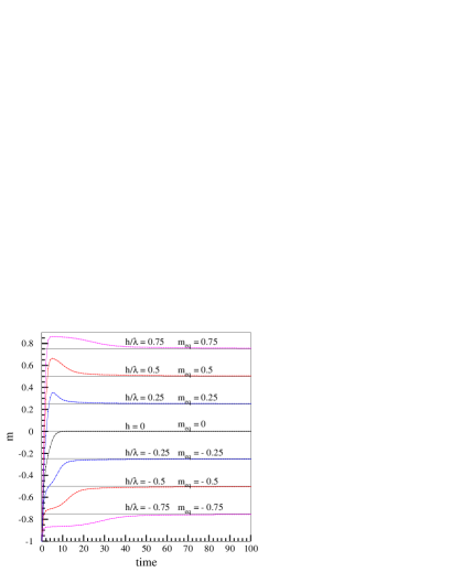
Figure 2: (Color online) Time evolution of the magnetization for different values of $h$, $\lambda=1$ and $T=0.25\,T_{C}(h)$.

Let us first consider $(T,h)$ in the region of phase separation, with $T<T_{C}(h)$. Fig. 2 and Fig. 3 illustrate quite well the considerations made at the end of the previous section. The first one displays the evolution of the magnetization for different values of $h$. After a fast transient there is saturation to the equilibrium value

$$m_{eq}={h\over\lambda}$$ (37)

taking place from above or from below for $h$ positive or negative, respectively. Apart from the details of the transient, this behavior of the magnetization agrees with the prediction and results of Ref. epl+FDGC+08 for the scalar model.

As explained above, when the magnetization gets stabilized at the value (37) by $h_{eff}=0$, the growth of the Bragg peak is inevitable in order to equilibrate the system. This is illustrated in Fig. 3. In the late time regime the structure factor is expected to obey a scaling form of the type Bra95

$$C_{\perp}(k,t)\sim L^{d}(t)F(kL(t)),$$ (38)

where $F(kL(t))$ is a scaling function and $L(t)\sim t^{1/z}$ with $z=2$, as appropriate for phase ordering processes without conservation of the order parameter, is a time dependent characteristic length nota2 . The same growth law $t^{1/2}$ was found in Ref epl+FDGC+08 for the mean cluster size. The inset of Fig. 3 shows that the height of the peak follows quite well the power law

$$C(k_{min},t)\sim t^{3/2}.$$ (39)

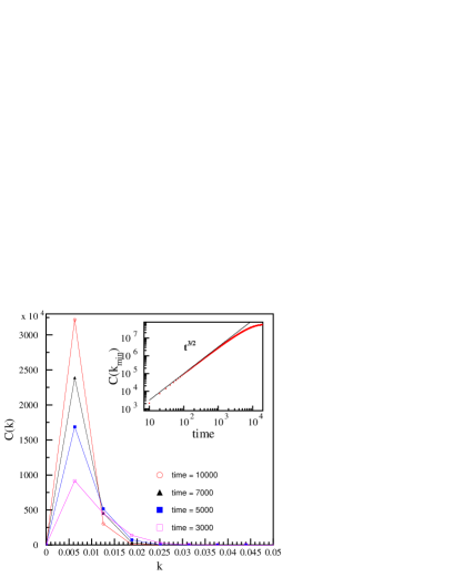
Figure 3: (Color online) Time evolution of the transverse structure factor $C_{\perp}(k,t)$ for $h=0.5$, $\lambda=1$ and $T=0.25T_{C}(h)$. Inset: time evolution of the peak height $C_{\perp}(k_{min},t)$

.

Actually, for times of order $10^{3}-10^{4}$ there appears a deviation from the power law (39). This is a finite size effect, unavoidable in the numerical computation and not to be confused with the equilibration of the magnetization, which is independent of the size of the system (notice the huge difference in the time scales). Therefore, considering the infinite system, we have the interesting instance of two observables in the same system, one of which (the magnetization) equilibrates rather quickly, while the other (the structure factor) does not reach equilibrium in any time scale.

Conversely, if $T>T_{c}(h)$ there is a solution of the self-consistency relation without growth of the condensate and both the magnetization and the structure factor reach equilibrium in the same time scale. This is illustrated in Fig. 4, displaying the saturation of the magnetization to the limit value $m_{eq}=\frac{h}{\lambda+\mu^{*}}$ with $\mu^{*}>0$, in agreement with Eq. (34), while the inset shows the saturation of the peak height to the equilibrium value

$$T/(k_{min}^{2}+\mu^{*})$$ (40)

in agreement with Eq. (35).

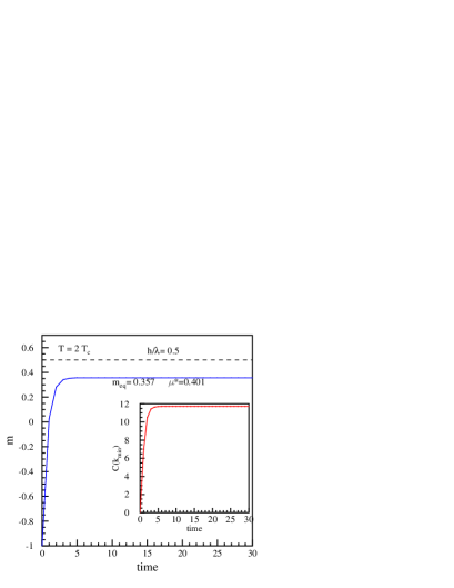
Figure 4: (Color online) Behavior of magnetization outside the coexistence region, with $h=0.5$, $\lambda=1$ and $T=2T_{C}(h)$. The dotted line represents the equilibrium value of magnetization for $T<T_{C}(h)$. Inset: time evolution of $C_{\perp}(k_{min},t)$.

The same qualitative behavior, that we have here illustrated in the $d=3$ case, is expected for any $d>2$. For $d=2$, due to the divergence in the denominator of Eq. (30), the critical temperature vanishes squeezing the coexistence region of Fig. 1 onto the vertical axis at $T=0$. Therefore, in the $d=2$ case condensation of fluctuations can be obtained only for $T=0$ and $|h|\leq h_{C}$.

V Summary

In this paper we have studied the static and dynamic properties of a system described by a free energy functional with a short-range ferromagnetic interaction and a long-range antiferromagnetic interaction, in presence of an external uniform magnetic field. The analysis has been carried out in the large $N$ limit. The scalar counterpart of this model is the lattice-gas Hamiltonian epl+FDGC+08 used to model the phenomenology of phase separation occurring in the inner part of cell surface during directional sensing. We have focussed on the phase ordering process taking place below the critical temperature, even in the in presence of the external magnetic field.

In particular, through the equations of motion for the magnetization and the transverse structure factor, we have highlighted how the competing interactions induce the self-tuning of the magnetization within the phase coexistence region. We have derived the phase diagram, which depends on the magnetic field and the strength of the antiferromagnetic coupling, showing that phase-separation is possible for a range of values of the external field. Taking the large $N$ limit it has been possible to derive analytically the dependence of the critical temperature on the magnetic field and on antiferromagnetic coupling $\lambda$. The phase diagram of Fig. 1 depicts in the $(T,h)$ plane the phase coexistence regions for different values of $\lambda$. The equilibrium value of magnetization $m_{eq}=h/\lambda$ is in agreement with the prediction and with the results obtained in the Monte Carlo simulation for a lattice gas system (Ref. epl+FDGC+08 ). The dynamics shows that the antiferromagnetic coupling combines with the magnetization to generate the effective magnetic $h_{eff}$ field, eventually vanishing within the coexistence region. While the magnetization equilibrates very quickly, the structure factor does not equilibrate on any time scale.

For $T<T_{C}(h)$ the relaxation process is characterized by the growth of a condensate in transverse structure factor at the most unstable wave vector $k=k_{min}$. The onset of condensation signals the occurrence of a phase separation and corresponds to domain coarsening in the scalar case. The late time behavior of the structure factor is characterized by dynamical scaling and power law growth of the peak, with the exponent $d/2$ characteristic of non conserved order parameter.

In conclusion, we have analyzed a model where the competition between the short-range ferromagnetic and the long-range antiferromagnetic interaction between two species leads to the phase separation for a wide range of external field and temperature. The occurrence of phase separation is a crucial intermediate step allowing for the amplification of external field gradients, leading to directional sensing as illustrated in Ref. epl+FDGC+08 .

The general property of the free energy functional (1), giving rise to phase coexistence through self-tuning, can be very useful in other contexts characterized by the balance between short range attraction, long-range repulsion and an overall external action.

Acknowledgements. MZ acknowledges financial support from MURST through the PRIN project 2007JHLPEZ Fisica Statistica dei Sistemi Fortemente Correlati all’Equilibrio e Fuori dall’Equilibrio: Risultati Esatti e Metodi di Teoria dei Campi.

References

- (1) M. Tarzia and A. Coniglio, Phys. Rev. E, 75, 011410 (2007).
- (2) A. Giuliani, J.Lebowitz and E.H.Lieb, arXiv: 0811.3078v1.
- (3) S. Bornholdt, Internal Jurnal of Modern Physics C, 12, 667 (2001).
- (4) B. Alberts, A. Jonson, J. Lewis, M. Raff, K. Roberts and P. walter, molecular Biology of the Cell, Garland Science, (2007).
- (5) C. Janetopoulos, Lan Ma, P. N. Devreotes, and P. A. Iglesias, P.N.A.S. U.S.A. 101, 8951 (2004).
- (6) A. Gamba, A. de Candia, S. Di Talia, A. Coniglio, F. Bussolino and G. Serini, P.N.A.S. U.S.A. 102, 16927 (2005).
- (7) M. Postma, J. Roelofs, J. Goedhart, H. M. Loovers, A. J. W. G. Visser and P. J. M. Van Haastert1, J. Cell. Sci. 117, 2925 (2004).
- (8) J. D. Gunton, M. San Miguel, P. S. Sahni, in Phase transition and critical phenomena, edited by C. Domb and J. L. Lebowitz, Academic London, Vol. 8, (1983).
- (9) C. Sagui and R. C. Desai, Phys. Rev. E, 49, 2225 (1994).
- (10) T. Ferraro, A. de Candia, A. Gamba and A. Coniglio, Europhysics Letters 83, 50009, (2008).
- (11) A. Gamba, I. Kolokolov, V. Lebedev and G. Ortenzi, J. Stat. Mech. P02019 (2009).
- (12) A. Gamba, I. Kolokolov, V. Lebedev and G. Ortenzi, Phys. Rev. Lett., 99, 158101 (2007).
- (13) S.H. Zigmond, J. Cell. Biol. 75, 606 (1977).
- (14) A. Coniglio, P. Ruggiero, and M. Zannetti, Phys. Rev. E, 50, 1046 (1994).
- (15) A. Bray, Adv. Phys. 45, 357 (1994).
- (16) In practice such a final state is never achieved, since an infinite system quenched below the critical point never equilibrates.
- (17) C. Castellano, F. Corberi and M. Zannetti, Phys. Rev. E, 56, 4973 (1997).
- (18) N.Fusco and M.Zannetti, Phys. Rev. E, 66, 066113 (2002).
- (19) A.Coniglio and M.Zannetti, Europhys. Lett. 10, 575 (1989).
- (20) J. Zinn-Justin, Quantum Field Theory and Critical Phenomena Chapter 30, Fourth Edition, Oxford University Press (2002).
- (21) More precisely, is the -dimensional solid angle over .
- (22) W. H. Press, B. P. Flannery, S. A. Teukolsky, W. T. Vetterling, Numerical Recipes in C: The Art of Scientific Computing, Second Edition, (1992).
- (23) In the case of non linear systems with a genuine phase ordering process is related to the size of coarsening domains.