A modified Ehrenfest formalism for efficient
large-scale ab initio molecular dynamics
Abstract
We present in detail the recently derived ab-initio molecular dynamics (AIMD) formalism [Phys. Rev. Lett. 101 096403 (2008)], which due to its numerical properties, is ideal for simulating the dynamics of systems containing thousands of atoms. A major drawback of traditional AIMD methods is the necessity to enforce the orthogonalization of the wave-functions, which can become the bottleneck for very large systems. Alternatively, one can handle the electron-ion dynamics within the Ehrenfest scheme where no explicit orthogonalization is necessary, however the time step is too small for practical applications. Here we preserve the desirable properties of Ehrenfest in a new scheme that allows for a considerable increase of the time step while keeping the system close to the Born-Oppenheimer surface. We show that the automatically enforced orthogonalization is of fundamental importance for large systems because not only it improves the scaling of the approach with the system size but it also allows for an additional very efficient parallelization level. In this work we provide the formal details of the new method, describe its implementation and present some applications to some test systems. Comparisons with the widely used Car-Parrinello molecular dynamics method are made, showing that the new approach is advantageous above a certain number of atoms in the system. The method is not tied to a particular wave-function representation, making it suitable for inclusion in any AIMD software package.
1 Introduction
In the last decades the concept of theoretical atomistic simulations of complex structures in different fields of research (from material science in general, to biology) has emerged as a third discipline between theory and experiment. Computational science is now an essential adjunct to laboratory experiments, it provides high-resolution simulations that can guide research and serve as tools for discovery. Today, computer simulations unifying electronic structure and ion dynamics have come of age, although important challenges remain to be solved. This “virtual lab” can provide valuable information about complex materials with refined resolution in space and time, allowing researchers to gain understanding about the microscopic and physical origins of materials behavior: from low-dimensional nano-structures, to geology, atmospheric science, renewable energy, (nano)electronic devices, (supra)molecular chemistry, etc. Since the numerical approaches to handle those problems require “large-scale calculations” the success of this avenue of research was only possible due to the development of high-performance computers333As stated by Dirac in 1929, “The fundamental laws necessary for the mathematical treatment of a large part of physics and the whole of chemistry are thus completely known, and the difficulties lies only in the fact that application of these laws leads to equations that are too complex to be solved”. The present work addresses our recent developments in the field of first-principles molecular dynamics simulations. Before getting into the details, we would like to frame properly the work from a historical perspective.
Molecular dynamics (MD)[1] consists of following the dynamics of a system of atoms or molecules governed by some interaction potential; in order to do so, “one could at any instant calculate the force on each particle by considering the influence of each of its neighbors. The trajectories could then be traced by allowing the particles to move under a constant force for a short-time interval and then by recalculating a new force to apply for the next short-time interval, and so on.” This description was given in 1959 by Alder and Wainwright[2] in one the first reports of such a computer-aided calculation444 Computer simulations of the dynamics of systems of interacting molecules based on the Monte Carlo methods were presented some years before[3]. Also, before the work of Alder and Wainwright, some previous ”computations” were reported that did not utilize modern computers, but rather real physical models of the system, i.e. rubber balls linked by rods[4]. The rapid improvement of digital computer machines discouraged this cumbersome, yet entertaining, methodology., though the first MD simulation was probably done by Fermi et al.[5, 6] for a one-dimensional model solid. We can still use this description to broadly define the scope of MD, although many variants and ground-breaking developments have appeared during these fifty years, addressing mainly two key issues: the limitation in the number of particles and the time ranges that can be addressed, and the accuracy of the interaction potential.
The former issue was already properly stated by Alder and Wainwright: “The essential limitations of the method are due to the relatively small number of particles that can be handled. The size of the system of molecules is limited by the memory capacity of the computing machines.” This statement is not obsolete, although the expression “small number of particles” has today of course a very different meaning – linked as it is to the exponentially growing capacities of computers.
The latter issue – the manner in which the atomic interaction potential is described – has also developed significantly over the years. Alder and Wainwright used solid impenetrable spheres in the place of atoms; nowadays, in the realm of the so-called “classical” MD one makes use of force fields: simple mathematical formulae are used to describe atomic interactions; the expressions are parameterized by fitting either to reference first-principles calculations or experimental data. These models have become extremely sophisticated and successful, although they are ultimately bound by a number of limitations. For example, it is difficult to tackle electronic polarization effects and one needs to make use of polarizable models, whose transferability is very questionable but are widely used with success in many situations. Likewise, the force field models are constructed assuming a predetermined bond arrangement, disabling the option of chemical reactions – some techniques exist that attempt to overcome this restriction[7], but they are also difficult to transfer and must be carefully adapted to each particular system.
The road towards precise, non-empirical inter-atomic potentials reached its destination when the possibility of performing ab initio MD (AIMD) was realized[8, 9]. In this approach, the potential is not modelled a priori via some parameterized expression, but rather generated “on the fly” by performing accurate first-principles electronic structure calculations. The accuracy of the calculation is therefore limited by the level of theory used to obtain the electronic structure – although one must not forget that underlying all MD simulations is the electronic-nuclear separation ansatz, and the classical limit for the nuclei. The use of very accurate first principles methods for the electrons implies very large computational times, and therefore it is not surprising that AIMD was not really born until density-functional theory (DFT) became mature – since it provides the necessary balance between accuracy and computational feasibility[10, 11, 12, 13]. Of fundamental importance was the development of gradient generalized exchange and correlation functionals, like the ones proposed by John Perdew[15, 16, 14], that can reproduce experimental results better than the local density approximation [18, 19, 17]. In fact, the whole field of AIMD was initiated by Car and Parrinello in 1985[20], in a ground-breaking work that unified DFT and MD, and introduced a very ingenious acceleration scheme based on a fake electronic dynamics. As a consequence, the term AIMD in most occasions refers exclusively to this technique proposed by Car and Parrinello. However, it can be understood in a more general sense, including more possibilities that have developed thereafter – and in the present work we will in fact discuss one of them. The new scheme proposed below will benefit from all the algorithm developments and progress being done in the CP framework.
As a matter of fact, the most obvious way to perform AIMD would be to compute the forces on the nuclei by performing electronic structure calculations on the ground-state Born-Oppenheimer potential energy surface. This we can call ground-state Born Oppenheimer MD (gsBOMD). It implies a demanding electronic minimization at each step and schemes using time-reversible integrators have been recently developed[22, 21]. The Car-Parrinello (CP) technique is a scheme that allows to propagate the Kohn-Sham (KS) orbitals with a fictitious dynamics that nevertheless mimics gsBOMD – bypassing the need for the expensive minimization. This idea has produced an enormous impact, allowing for successful applications in a surprisingly wide range of areas (see the special number in ref. 23 and references therein). Still, it implies a substantial cost, and many interesting potential applications have been frustrated due to the impossibility of attaining the necessary system size or simulation time length. There have been several efforts to refine or redefine the CP scheme in order to enhance its power: linear scaling methods[24] attempt to speed-up in general any electronic structure calculation; the use of a localized orbital representation (instead of the much more common plane-waves utilized by CP practitioners) has also been proposed[25]; recently, Kühne and coworkers[26] have proposed an approach which is based on CP, but which allows for sizable gains in efficiency. In any case, the cost associated with the orbital orthonormalization that is required in any CP-like procedure is a potential bottleneck that hinders its application to very large-scale simulations.
Another possible AIMD strategy is Ehrenfest MD, to be presented in the following section. In this case, the electron-nuclei separation ansatz and the Wentzel-Kramers-Brillouin[27, 28, 29] (WKB) classical limit are also considered; however, the electronic subsystem is not assumed to evolve on only one of the electronic adiabatic states – typically the ground-state one. Instead the electrons are allowed to evolve on an arbitrary wave-function that corresponds to a combinations of adiabatic states. As a drawback, the time-step required for a simulation in this scheme is determined by the maximum electronic frequencies, which means about three orders of magnitude less than the time step required to follow the nuclei in a BOMD.
If one wants to do Ehrenfest-MD, the traditional “ground-state” DFT is not enough, and one must rely on time-dependent density-functional theory (TDDFT)[30, 31]. Coupling TDDFT to Ehrenfest MD provides with an orthogonalization-free alternative to CP AIMD – plus it allows for excited-states AIMD. If the system is such that the gap between the ground-state and the excited states is large, Ehrenfest-MD tends to gsBOMD. The advantage provided by the lack of need of orthogonalization is unfortunately offset by the smallness of the required time-step[18, 8]. Recently, some of the authors of the present article have presented a formalism for large scale AIMD based on Ehrenfest and TDDFT, that borrows some of the ideas of CP in order to increase this time step and make TDDFT-Ehrenfest competitive with CP[32].
This article intends to provide a more detailed description of this proposed methodology: we start, in Section 2 by revisiting the mathematical route that leads from the full many-particle electronic and nuclear Schrödinger equation to the Ehrenfest MD model. Next, we clear up some confusions sometimes found in the literature related to the application of the Hellmann-Feynman theorem, and we discuss the integration of Ehrenfest dynamics in the TDDFT framework. Section 4 presents in detail the aforementioned novel formalism, along with a discussion regarding symmetries and conservation laws. Sections 5 and 6 are dedicated to the numerical technicalities, including several application examples.
2 Ehrenfest dynamics: fundaments and implications for first principles simulations
The starting point is the time-dependent Schrödinger equation (atomic units [33] are used throughout this paper) for a molecular system described by the wave-function :
| (2.1) |
where the dot indicates the time derivative, and we denote as , , and , the Euclidean coordinates and the spin of the -th electron and the -th nuclei, respectively, with , and . We also define , and , and we shall denote the whole sets , , , and , using single letters in order to simplify the expressions.
The non-relativistic molecular Hamiltonian operator is defined as
| (2.2) | |||||
where all sums must be understood as running over the whole natural set for each index, unless otherwise specified. is the mass of the -th nucleus in units of the electron mass, and is the charge of the -th nucleus in units of (minus) the electron charge. Also note that we have defined the nuclei-electrons potential and the electronic Hamiltonian operators.
Now, in order to derive the quantum-classical molecular dynamics (QCMD) known as Ehrenfest molecular dynamics from the above setup, one starts with a separation ansatz for the wave-function between the electrons and the nuclei [34, 35], leading to the so-called time-dependent self-consistent-field (TDSCF) equations [8, 36, 37]. The next step is to approximate the nuclei as classical point particles via short wave asymptotics, or WKB approximation [8, 27, 28, 29, 36, 37]. The resultant Ehrenfest MD scheme is contained in the following system of coupled differential equations [36, 37]:
| (2.4a) | ||||
| (2.4b) | ||||
where is the wave-function of the electrons, are the nuclear trajectories, and we have used to indicate integration over all spatial electronic coordinates and summation over all electronic spin degrees of freedom. Also, a semicolon has been used to separate the from the in the electronic Hamiltonian, in order to stress that only the latter are actual time-dependent degrees of freedom the system.
The initial conditions in Ehrenfest MD are given by
| (2.5a) | ||||
| (2.5b) | ||||
and we assume that vanishes at infinity .
Also note that, since in this scheme is a set of independent variables, we can rewrite eqs. (2.4b) as
| (2.6) |
a fact which is similar in form, but unrelated to the Hellmann-Feynman theorem555 Perhaps the first detailed derivation of the so-called Hellmann-Feynman theorem was given in Güttinger, P. Z. Phys. 1931, 73, 169-184. The theorem had nevertheless been used before that date.[38] The derivations of Hellmann[39] and Feynman[40], who named the theorem, came a few years afterwards.. As pointed out by Tully [41], it is likely that the confusion about whether eqs. (2.6) should be used to define the Ehrenfest MD, or the gradient must be applied to the electronic Hamiltonian inside the integral, as in (2.4b), has arisen from applications in which is expressed as a finite expansion in the set of adiabatic basis functions, , defined as the eigenfunctions666In general, may contain a discrete and a continuous part. However, in this manuscript, we will forget the continuous part in order to simplify the mathematics. of :
| (2.7) |
The use of a precise notation, such as the one introduced in this section, helps to avoid this kind of confusions. An example of a misleading notation in this context would consist in writing for the electronic wave-function [41, 42], when, as we have emphasized, there exists no explicit dependence of on the nuclear positions .
In Ehrenfest MD transitions between electronic adiabatic states are included. This can be made evident by performing the following change of coordinates from to (with ):
| (2.8a) | |||||
| (2.8b) | |||||
where are known functions given by (2.7) and, even if the transformation between the and the is trivial, we have used the prime to emphasize that there are two distinct sets of independent variables: and . This is very important if one needs to take partial derivatives, since a partial derivative with respect to a given variable is only well defined when the independent set to which that variable belongs is specified777 In the development of the classical formalism of Thermodynamics, this point is crucial.. For example, a possible mistake is to assume that, since ‘is independent of’ , and , then ‘is also independent’ of and, therefore, the unprimed partial derivative is zero. The flaw in this reasoning is that the unprimed partial derivative is defined to be performed at constant , and not at constant , since the relevant set of independent variables is . In fact, if we write the inverse transformation
| (2.9a) | |||||
| (2.9b) | |||||
we can clearly appreciate that, even if it is independent from by construction, is neither independent from , nor from 888 This mistake is made, for example, in ref. 42 when going from their expression (8) to their expression (9). Having not realized the existence of the two distinct sets of independent variables: and , they treat the as constants when taking the partial derivative with respect to (our ) at the right hand side of (8), thus arriving to (9), where the cross-terms , with , are incorrectly missing (see the correct derivation of EMD in the adiabatic basis below). . On the other hand, if we truncated the sum in (2.8a), then there would appear an explicit dependence of on and the state of affairs would be different, since would no longer be a set of independent variables. However, in the context of an exact (infinite) expansion in (2.8a), the right hand sides of eqs. (2.4b) and (2.6) are equal, as we mentioned before, and we do not have to worry about which one is more appropriate. It is in this infinite-adiabatic basis situation that we will now use eq. (2.4b) and the expansion in (2.8a) to illustrate the non-adiabatic character of Ehrenfest MD.
If we perform the change of variables described in eqs. (2.8) to the Ehrenfest MD eqs. (2.4), and we use that
| (2.10) |
we see that we will have to calculate terms of the form
| (2.11) |
which can be easily extracted from the relation
| (2.12) |
In this way, we obtain for the nuclear Ehrenfest MD equation
| (2.13) | |||||
where the non-adiabatic couplings (NACs) are defined as
| (2.14) |
To obtain the new electronic Ehrenfest MD equation, we perform the change of variables to (2.4a) and we then multiply by the resulting expression and integrate over the electronic coordinates . Proceeding in this way, we arrive to
| (2.15) |
In the nuclear eqs. (2.13), we can see that the term depending on the moduli directly couples the population of the adiabatic states to the nuclei trajectories, whereas interferences between these states are included via the contributions. Analogously, in the electronic equations above, the first term represents the typical evolution of the coefficient of an eigenstate of a Hamiltonian, but, differently from the full quantum case, in Ehrenfest MD, the second term couples the evolution of all states with each other’s through the velocity of the classical nuclei and the NACs.
Moreover, Ehrenfest MD is fully (quantum) coherent, since the complex coefficients , are the ones corresponding to the quantum superposition in the electronic wave function. A proper theory that treats realistically the electronic process of coherence and decoherence is of fundamental importance to properly interpret transition rates and to have control over processes happening at the attosecond/femtosecond time scales, such as the description of the optimal-pulse laser (in optimal control theory) that enhances a given channel in a chemical reaction, the manipulation of qbits in quantum computing devices, the generation of soft X-rays by high-harmonic generation, or the energy transfer processes in photosynthetic units [43].
At finite temperature, it is known that Ehrenfest MD cannot account for the Boltzmann equilibrium population of the quantum subsystem [44, 45, 46]. The underlying reason of this failure is the mean field approximation in eq. (2.4b) which neglects the nuclei response to the microscopic fluctuations in the electronic charge density.
In order to address this point, it is important to distinguish between two different physical situations considered in the literature for studying equilibrium within Ehrenfest: In ref. 44, a mixed quantum-classical system is coupled, only via the classical degrees of freedom, to a classical bath. The dissipative dynamics is integrated using a Nosé thermostat, while the mixed quantum-classical one is integrated using Ehrenfest. In ref. 45, 46, on the other hand, the classical degrees of freedom are the bath to which the quantum system is coupled, i.e., the thermalization of a quantum system due to its “Ehrenfest-like” coupling to a bath or solvent is discussed. Only the first of these two approaches corresponds to the physical problem we want to deal with, namely, the thermalization of a mixed quantum-classical molecule in a bath.
Once the aforementioned drawback has been recognized, some authors have proposed several patches to ensure the Boltzmann population equilibrium for the quantum subsystem: In Tully’s surface hopping (SH) method [47], the quantum degrees of freedom also follow eq. (2.4a), however, instead of the mean-field dynamics (2.4b), the classical degrees of freedom follow a stochastic-like equation describing jumps between adiabatic states. Unfortunately, this method does not give in general the desired equilibrium averages either [48], and it looses the physical meaning of time during propagation.
Another new method by Bastida and collaborators [49, 50], proposes an ad-hoc modification of the Ehrenfest equations in order to obtain the correct equilibrium distribution of a quantum system coupled to a classical bath, i.e., the classical degrees of freedom are the solvent for the quantum system. Their idea can be summarized as follows: Expressing in (2.15) the complex coefficients in polar form (), and writing the equations for the moduli, one obtains , where we have used the compact notation: , cf. eq. (2.15). Analogous equations are derived for the phases . Written like this, the equations are formally similar to balance-like equations for the diagonal elements of the density matrix of the quantum system in the adiabatic basis. These kinetic equations have been extensively studied in relaxation processes, and it is known that, to ensure equilibrium, the coefficients, , must fulfill the detailed-balance condition, i.e., , with being the energy difference between the and states[51]. The proposal by Bastida et al.[49, 50] proceeds by defining some modified transition coefficients , such that detailed balance is enforced, an thus approaching the Boltzmann equilibrium population for the quantum system.
Coming back to the situation discussed in ref. 44, i.e., where the classical subsystem is not a bath, but a part of the mixed quantum-classical system coupled to a reservoir, one can go beyond Ehrenfest and make use of the formalism developed in refs. 52, 53, 54. The description in these works is not mean-field, and the quantum-classical dynamics is treated exactly. Although its practical implementation seems cumbersome, it is a path to explore, with possible modifications, in the near future.
3 Ehrenfest-TDDFT
TDDFT offers a natural framework to implement Ehrenfest MD. In fact, starting by an extension [56] of the Runge-Gross theorem [57] to arbitrary multicomponent systems, one can develop a TDDFT [58] for the combined system of electrons and nuclei described by (2.1). Then, after imposing a classical treatment of nuclear motion, one arrives to an Ehrenfest-TDDFT dynamics. This scheme can also be generated from the following Lagrangian [58, 59, 32]:
| (3.1) | |||||
where we have denoted by , the whole set of Kohn-Sham (KS) orbitals of a closed-shell molecule, and is the KS energy:
| (3.2) | |||||
where is the exchange-correlation energy, and the time-dependent electronic density is defined as
| (3.3) |
In the following section, we introduce a modification of the Ehrenfest-TDDFT dynamics obtained from (3.1) aimed to the study of situations in which the contribution of the electronic excited states to the nuclei dynamics is negligible, i.e., situations in which one is interested in performing ground-state Born-Oppenheimer molecular dynamics (gsBOMD) [8].
4 Modified Ehrenfest-TDDFT formalism
4.1 Lagrangian and equations of motion
We now introduce the basic concepts and approximations that define the new fast Ehrenfest-TDDFT dynamics framework that some of the authors introduced in ref. 32. The new scheme can be obtained from the following Lagrangian
| (4.1) |
Note that the major modification with respect to the Ehrenfest-TDDFT Lagrangian in eq. (3.1) is the presence of a parameter that introduces a re-scaling of the electronic velocities (Ehrenfest-TDDFT is recovered when ). The equations of motion of the new Lagrangian, eq. (4.1), are:
| (4.2a) | |||||
| (4.2b) | |||||
where is the time-dependent KS effective potential. As we are interested in the adiabatic regime, we will restrict the exchange and correlation potential to depend only on the instantaneous density (in general the exchange correlation potential in TDDFT depends on the density of all previous times, although for practical calculation this same adiabatic approximation is done).
Compare with the gsBOMD Lagrangian:
| (4.3) |
and the corresponding equations of motion:
| (4.4a) | |||||
| (4.4b) | |||||
| (4.4c) | |||||
where is a Hermitian matrix of time-dependent Lagrange multipliers that ensure that the orbitals form an orthonormal set at each instant of time. The Euler-Lagrange equations corresponding to in (4.4b) are exactly these orhonormality constraints, and, together with eq. (4.4a), constitute the time-independent KS equations. Therefore, assuming no metastability issues in the optimization problem, the orbitals are completely determined999 This fact is not in contradiction with the above discussion about coordinates independence. The difference between Ehrenfest MD and gsBOMD is that in the Lagrangian for the latter, the orbitals ‘velocities’ do not appear, thus generating Eqs. (4.4a) and (4.4b), which can be regarded as constraints between the and the . by the nuclear coordinates , being in fact the BO ground state (gs), , which allows us to write the equations of motion for gsBOMD in a much more compact and familiar form:
| (4.5) |
We can also compare the dynamics introduced in eqns. (4.2) with CPMD, whose Lagrangian reads
| (4.6) | |||||
and the corresponding equations of motion are
| (4.7a) | |||||
| (4.7b) | |||||
| (4.7c) | |||||
where is again a Hermitian matrix of time-dependent Lagrange multipliers that ensure the orthonormality of the orbitals , and is a fictitious electrons ‘mass’ which plays a similar role to the parameter in our new dynamics.
Before discussing in details the main concepts of the present dynamics it is worth to state its main advantages and deficiencies (that will be the topic of discussion in the next sections). When applied to perform gsBOMD the method can gain a large speed-up over Ehrenfest MD, it preserves exactly the total energy and the wave-function orthogonality, and allows for a very efficient parallelization scheme that requires low communication. However, the speed-up comes at a cost as it increases the non-adiabatic effects. Also, the method as discussed above will not work properly for metals and small-gap systems101010We are exploring how to overcome this limitation by mapping the real Hamiltonian into another one that produces the same dynamics but not having contributions from the empty states..
4.2 Symmetries and conserved quantities
In the following we will study the conserved quantities associated to the global symmetries of the Lagrangian in eq. (4.1) and we shall compare them with those of gsBOMD and CPMD. We will also be interested in a gauge symmetry that is the key to understand the behaviour of eq. (4.1) in the limit and its relation with gsBOMD.
The first symmetry we want to discuss is the time translation invariance of (4.1). This is easily recognized as does not depend explicitly on time. Associated to this invariance there is a conserved ‘energy’. Namely, using Noether theorem we have that
| (4.8) |
is constant under the dynamics given by eq. (4.2), where indexes the Euclidean coordinates of vectors (and if needed).
Notice that does not depend on the unphysical parameter and actually coincides with the exact energy that is conserved in gsBOMD. The situation is different in CPMD. There, we also have time translation invariance but the constant of motion reads
| (4.9) |
which depends directly on the unphysical ‘mass’ of the electrons, , and its conservation implies that the physical energy varies in time. Still, this drawback has a minor effect, since it has been shown that the CP physical energy follows closely the exact gsBOMD energy curve.
The second global symmetry we want to consider is the change of orthonormal basis of the space spanned by . Namely, given a Hermitian matrix (), we define the following transformation:
| (4.10) |
The Lagrangian in (4.1) depends on only through and . Provided the matrix is Hermitian and constant in time, both expressions are left unchanged by the transformation. Hence, we can invoke again Noether theorem to obtain a new conserved quantity that reads
| (4.11) |
Observe that we have a constant of motion for any Hermitian matrix . This permits us to combine different choices of in order to obtain that
| (4.12) |
In other words, if we start with an orthonormal set of wave functions and we let evolve the system according to equations (4.2), the family of wave functions maintains its orthonormal character along time, i.e. the operator preserves the inner product of the wave-functions that define the Ehrenfest trajectory.
We would like to mention here that the above property is sometimes substantiated on a supposed unitarity of the evolution operator. [8, 59, 60]. Simply noticing that the evolution of is not linear as both (4.2a) and (4.2b) are non-linear equations, and that unitary evolution requires linearity 111111For a one to one transformation we may define unitarity as the property of preserving the scalar product, i. e. given two arbitrary vectors and we have . One can easily see that any reversible transformation that enjoys the previous property is necessarily linear: As is reversible, is an arbitrary vector, and therefore we must have Hence as the equations of motion (4.2a) and (4.2b) are clearly non linear, the evolution is non linear too and consequently it can not be a unitary transformation as defined above. If we fix the value of the density for all times, then the operator will become linear and it will be unitary., one can discard from the start the unitarity argument.
There is however a delicate point here that is worth discussing. The issue is that the limit of our dynamics should correspond to gsBOMD in eqns. (4.4) (which includes Lagrange multipliers to keep orthonormalization), but the Lagrangian in (4.1) does not contain any multipliers and in fact they are unnecessary, as our evolution preserves the orthonormalization. This may rise some doubts on the equivalence between gsBOMD and the limit of vanishing of our dynamics.
To settle the issue we introduce the additional dynamical fields , corresponding to Lagrange multipliers, in our Lagrangian in eq. (4.1), i.e.,
| (4.13) |
This modification has an important consequence: the global symmetry in (4.10) becomes a gauge one with time-dependent matrix elements. Actually one can easily verify that is invariant under
| (4.14a) | ||||
| (4.14b) | ||||
This implies that, for , the fields can be transformed to any desired value by suitably choosing the gauge parameters . Their value is therefore irrelevant and one could equally well take , as in (4.1), or (the value it has in gsBOMD) without affecting any physical observable. This solves the puzzle and shows that the limit of the dynamics of eq. (4.2) is in fact the exact gsBOMD.
Physical interpretation
If we take equation (4.2a) and write the left hand side as
| (4.15) |
the resulting equation can be seen as the standard Ehrenfest method in terms of a fictitious time . Two important properties can be obtained from this transformation.
On the one hand, it is easy to see that the effect of is to scale the TDDFT () excitation energies by a factor. So for the gap of the artificial system is decreased with respect to the real one, while for small values of , the excited states are pushed up in energy forcing the system to stay in the adiabatic regime. This gives a physical explanation to the limit shown before.
On the other hand, given the time step for standard Ehrenfest dynamics, , from (4.15) we can obtain that the time step as a function of is
| (4.16) |
so, for propagation will be times faster than Ehrenfest.
By taking into account these two results we can see that there is a trade-off in the value of : low values will give physical accuracy while large values will produce a faster propagation. The optimum value, that we will call , is the maximum value of that still keeps the system near the adiabatic regime. It is reasonable to expect that this value will be given by the ratio between the electronic gap and the highest vibrational frequency in the system. For many systems, like some molecules or insulators, this ratio is large and we can expect large improvements with respect to standard Ehrenfest MD. For other systems, like metals, this ratio is small or zero and our method will not work well without modifications (that are presently being worked on). We note that a similar problem appears in the application of CP to these systems.
4.3 Numerical properties
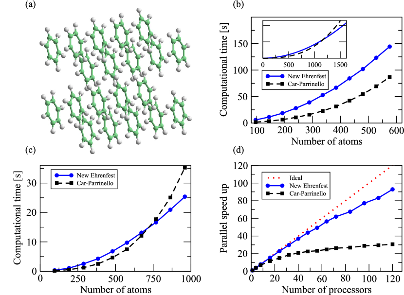
From the numerical point of view our method inherits the main advantage of Ehrenfest dynamics: since propagation preserves orthogonality of the wave-function, it needs not be imposed and the numerical cost is proportional to (with the number of orbitals and the number of grid points or basis set coefficients). For CP a re-orthogonalization has to be done each time step, so the cost is proportional to . From these scaling properties we can predict that for large enough systems our method will be less costly than CP. As we will show below this crossing can occur for around 1000 atoms for our implementation and the systems we have considered.
Due to the complex nature of the propagator, Ehrenfest dynamics has to be performed using complex wave-functions. In CP real wave-functions can be used if the system is finite (without a magnetic field) or if the system is a supercell using only the gamma point. However, with respect to CP, the actual number of degrees of freedom to be treated is the same, since CP equations are second order a second field has to be stored, either the artificial “velocity” of the wave-functions or the wave-function of the previous step.
An important point of comparison between Ehrenfest and CP is the dependency of the maximum time step with the simulation parameters: , and the cutoff energy (). While for our modified Ehrenfest scheme it will scale like
| (4.17) |
for CP dynamics we have that[8]
| (4.18) |
Since and are different quantities we cannot infer anything without knowing the effect of their value in the results, but as we will see from our calculations, even though in the new scheme the time step increases linearly with , the separation from the BO surface is also more sensitive to its value. On the other hand, the dependence with the cutoff energy is one of the major drawbacks of Ehrenfest dynamics, and probably it can explain why, as we will see, it is slower than CP for small systems. However in most cases this cutoff energy is independent from the size of the system and will only represent a difference in the prefactor in the scaling of both methods, so its effect should be compensated for large systems.
5 Methods
The scheme described above was implemented in the Octopus code[61, 62]. Octopus is general purpose code to handle equilibrium and non-equilibrium phenomena using (TD)DFT. It can be used to simulate atoms, molecules, low dimensional systems, and periodic structures under the presence of arbitrary electromagnetic fields. The code is distributed under a free software license and many new features are incorporated regularly. Octopus uses a real-space grid representation combined with the finite differences approximation for the calculation of derivatives[63, 64]. The nuclei-electron interaction is replaced by norm-conserving Troullier Martins pseudo-potentials. Unless stated otherwise the Perdew-Zunger[65] parametrization of the Local Density Approximation (LDA) is used for the exchange and correlation functional. The Poisson equation is solved using the interpolating scaling functions method[66].
5.1 Time-propagation
Given an initial condition and , we want to calculate and for a time from (4.2). For the ionic part, eq. (4.2b), once the forces are computed121212In principle the forces acting over the ions are given by eq. (4.2b), however, due to the derivatives of the ionic potential (that can have very high Fourier components), this expression is difficult to calculate accurately on real-space grids. Fortunately an alternative expression in terms of the gradient of the wave-functions can be obtained for both the local and non-local parts of the pseudo-potential[64]., the Newton equations can be handled easily by the standard velocity Verlet algorithm.
For the electronic part, eq. (4.2a), the transformation in eq. (4.15) allows us to use the standard Ehrenfest propagation methods, making our scheme trivial to implement in an existing real-time Ehrenfest code. The key part for the real-time solution of equation (4.2a) is to approximate the propagation operator
| (5.1) |
in an efficient and stable way. From the several methods available (see ref. 67 for a review), in this work we have chosen the approximated enforced time-reversal symmetry (AETRS) method. For a Hamiltonian , in AETRS the propagator is approximated by the explicitly time-reversible expression
| (5.2) |
with obtained from an interpolation from previous steps. For the calculation of the exponential in eq. (5.2) a simple fourth order Taylor expansion is used. Note that the truncation to any order of the Taylor expansion for the exponential operator implies that the norm of the vector is no longer conserved. This theoretical error must be kept below an acceptable threshold in order to ensure the preservation of the orthonormality of the orbitals. In any case, a small inevitable error will always lead to a slight change in the norm. If the norm is reduced, the method is said to be “contractive” – this property is desirable since it leads to stable propagations, as opposed to the case in which the norm increases: in this latter case the propagation becomes unstable. The choice for a fourth order truncation is advantageous because it is, for a very wide range of time-steps, a contractive approximation to the exponential.
Moreover, the careful preservation of time reversibility is crucial to avoid unphysical drifts in the total energy. We have found (for the cases presented in this work and for our particular numerical implementation) the combination of the AETRS approximation to the propagator together with the Taylor expansion representation of the exponential, to be the most efficient approach. Our tests show that numerically the error in orthonormality, measured as the dot product between orbitals, has an oscillatory behaviour and it is typically of the order of but for some pairs of orbitals it can increase to .
We also implemented the Car-Parrinello scheme to compare it with our approach. In this case the electronic part is integrated by the RATTLE/Velocity Verlet algorithm as described in ref. 68.
5.2 Parallelization strategy
The challenge of AIMD of going towards very large systems and large simulation times is clearly linked to implementations that run efficiently in parallel architectures. This is the case of CP methods, that are known to perform very well in this kind of systems[69, 70], the parallelization is usually based on domain decomposition (known as parallelization over Fourier coefficients in plane-wave codes) and K-points. However, good scalability can only be obtained if the system is large enough to have favorable computation-communication ratio with respect to the latency of the interconnection.
This type of parallelization is also applicable to the present Ehrenfest dynamics and, on top of that, the new scheme can add a different level of parallelization: since the propagation step is independent for each orbital, it is natural to parallelize the problem by distributing the Kohn-Sham states among processors. Communication is only required once per time-step to calculate quantities that depend on a sum over states: the time dependent densities and the forces over the ions. This type of sum of a quantity over several nodes is known as a reduction and the communication cost grows logarithmically with the number of nodes.
The main limitation to the parallel scalability in our real space implementation was observed to come from the parts of the code that do not depend on the states (global quantities), mainly the re-generation of the ionic potential
| (5.3) |
and the calculation of the forces due to the local part of the ionic potential
| (5.4) |
As these expressions depend on the atoms index a complementary parallelization in atoms is used to speed-up these code sections. For example, to generate the ionic potential, each processor generates the potential for a subset of the atoms and then a reduction operation is performed to obtain the total ionic potential.
Once this auxiliary parallelization over atoms is taken into account, it results in a very efficient scheme, similar to K-point parallelization for periodic systems, where, as long as there are enough states to distribute, the scaling is linear even with slow interconnections (as a rule of thumb, for our implementation 10-15 orbitals per processor are required for a good efficiency). In the case of CP, due to orthogonalization between states the evolution is not independent, so this parallelization scheme is more complex to implement and requires more communication, making it much less practical.
In our implementation we have combined this parallelization over states with real space domain decomposition (see ref. 62 for details). This dual parallelization strategy also has the advantage that allows us to decompose the two levels of complexity, the size of the region of space simulated and the number of orbitals, that increase when we move to study larger systems.
Below we address the relative gain in performance of the code once this second level of parallelization is used. To avoid as much as possible issues related to different software packages we decided to implement the two schemes, CP and Ehrenfest, in the same code. Although this might not be the the best parallel implementation of CP that is available in the community, it allows a direct assessment of the impact of this extra level of parallelization. Given the simplicity and the high level nature of parallelization over states, it is expected that this gain will be transferable to other implementations.
6 Applications: model and realistic systems
6.1 Two band model
To illustrate the properties of the new scheme, and also to compare it to CP in a complementary manner to the calculations in the rest of the manuscript, we apply it to a model system. The simple toy model we use is based on the one used in the work by Pastore et al. to test CP [71]. Its equations of motion are produced by the Lagrangian
| (6.1) | |||||
where and correspond to electronic degrees of freedom, to the nuclear motion and mimicks the gap. The parameters , , and have been taken from the experimental values for the N2 molecule (interpreting as the length of the N–N bond).
The dynamics produced by (6.1) has been then compared to the analogous CP one [obtained by simply changing the -kinetic energy by ], and to the gsBO reference [defined by setting , and and to the values that minimize the potential energy in (6.1), ]. In all simulations, the initial conditions of and have been increased a 10% from their equilibrium values and , we have set , and the initial electronic coordinates have been placed at the gsBO minimum (for CP, ).
To compare the approximate nuclear trajectory to the gsBO one , we define , where is the maximum variation of in the gsBO case. In 6.1a, we show that this distance smoothly decreases to zero as for our model. In 6.1b, in turn, we compare the gsBO force on to the one obtained from the new method averaging over a intermediate time between those associated to the electronic and nuclear motions. The distance between these forces (defined analogously to ), also goes to zero when .
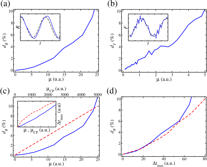
Now, we estimate the relation between the maximum time step allowed by the fourth order Runge-Kutta numerical integration of the equations of motion and the error, given by . The first, denoted by , has been defined as the largest time step that produced trajectories for all the dynamical variables of the system with a distance less than 0.1% to the ‘exact’ trajectories. In 6.1c, we can see that, although grows more slowly in our method than in CP (as expected from the discussion in section 4.3), the behaviour of the error () is better for the new dynamics introduced here. These two effects approximately balance each other yielding the error/time step relations depicted in 6.1d, where the new scheme is shown to behave similarly to CPMD for a significant range of values of . We stress however that, to actually compare the relative performance of both methods the numerical work required in each time step would have to be considered. In this sense, the more realistic simulations in the next sections are more representative.
6.2 Nitrogen molecule
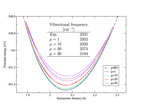
For the Nitrogen molecule (N2), we calculate the trajectories for different values of , using the same initial conditions as in the toy model. A time step of [fs] is used and the system is propagated by [fs]. In 6.2 we plot the potential energy as a function of the interatomic distance during the trajectory for each run, in the inset we also give the vibrational frequency for the different values of , obtained as the position of the peak in the Fourier transform of the velocity auto-correlation function. It is possible to see that for the simulation remains steadily close to the BO potential energy surface and there is only a deviation of the vibrational frequency. For the system starts to strongly separate from the gsBO surface as we start to get strong mixing of the ground state BO surfaces with higher energy BO surfaces. This behaviour is consistent with the physical interpretation given in section 4.2 as for this system .
6.3 Benzene
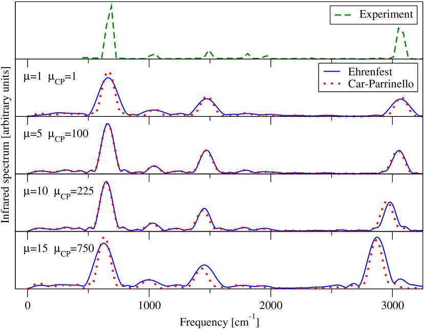
Next, we applied the method to the Benzene molecule. We set-up the atoms in the equilibrium geometry with a random Maxwell-Boltzmann distribution for . Each run was propagated for a period of time of [fs] with a time step of [fs] (that provide a reasonable convergence in the spectra). Vibrational frequencies were obtained from the Fourier transform of the velocity auto-correlation function. In table 1, we show some low, medium and high frequencies of Benzene as a function of . The general trend is a red-shift of the frequencies with a maximum deviation of 7 for . Still, to make a direct comparison with experiment, we computed the infrared spectra as the Fourier transform of the electronic dipole operator. In 6.3, we show how the spectra changes with . For large , besides the red-shift, spurious peaks appear above the higher vibrational frequency (not shown), this is probably due to non-adiabatic effect as is we consider the first virtual TDDFT excitation energy. We performed equivalent CP calculations for different values of , and found that, as shown in 6.3, it is possible to relate the physical error induced in both methods and establish and a relation between and .
| 398 | 961 | 1209 | 1623 | 3058 | |
| 396 | 958 | 1204 | 1620 | 3040 | |
| 391 | 928 | 1185 | 1611 | 2969 | |
| 381 | 938 | 1181 | 1597 | 2862 |
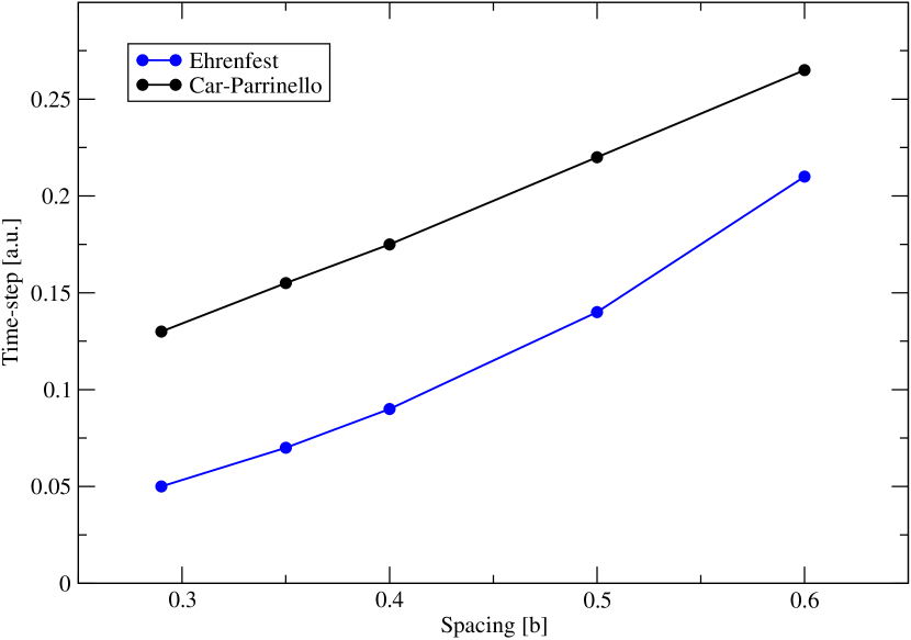
Having established the link between and we address the numerical performance of our new method compared to CP. As explained in section 4.3 the maximum time step has a different behaviour with the cutoff energy or equivalently, in this case, the grid spacing (the spacing is proportional to ). This can be seen in 6.4, where we plot the maximum time step both Ehrenfest and CP as a function of the grid spacing. This is important since, in order to be able to do a comparison for large number of atoms we use a larger spacing (0.6 [b] or 14 [Ha]) than the required for the converged results previously shown (0.35 [b] or 40 [Ha]). So for the small spacing case Ehrenfest results should be scaled by a 1.7 factor, these two values gives us a range of comparison, since most calculations are performed in this range of precision (14 [Ha] to 80 [Ha]).
To compare in terms of system size, we simulated several Benzene molecules in a cell. For the new scheme, a value of is used while for CP , (values that yield a similar deviation from the BO surface, according to 6.3). The time steps used are [a.u] and [a.u.] respectively. The computational cost is measured as the simulation time required to propagate one atomic unit of time, this is an objective measure to compare different MD schemes. We performed the comparison both for serial and parallel calculations; the results are shown in 6.5. In the serial case, CP is 3.5 times faster for the smaller system, but the difference reduces to only 1.7 times faster for the larger one. Extrapolating the results we predict that the new dynamics will become less demanding than CP for around 1100 atoms, if we consider the small spacing the crossover point moves to 2000 atoms. In the parallel case, the performance difference is reduced, being CP only 2 times faster than our method for small systems, and with a crossing point below 750 atoms (1150 atoms with the smaller spacing). This is due to the better scalability of the Ehrenfest approach, as seen on 6.5c. Moreover, in our implementation memory requirements as for our approach are lower than for CP: in the case of 480 atoms the ground state calculation requires a maximum of 3.5 Gb whereas in the molecular dynamics, Ehrenfest requires Gb while CP Gb. The scaling of the memory requirements is the same for both methods and we expect this differences to remain proportional for all system sizes.
6.4 Fullerene molecule: C60
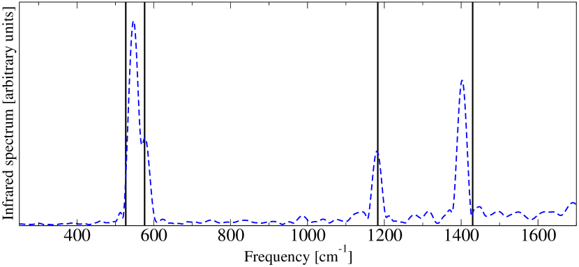
To end the computational assessment of the new formalism, we illustrate out method for the calculation of the infrared spectrum of a prototype molecule, C60. This time we switch to the PBE[14] exchange and correlation functional since it should give slightly better vibrational properties than LDA[17]. For the simulation shown below we use a value of that provides a reasonable convergence in the spectra. The calculated IR spectra is in very good agreement with the experiment (see 6.6) for low and high energy peaks (the ones more sensitive to the values of as seen in 6.3). The result is robust and independent of the initial condition of the simulation. The low energy splitting of IR spectrum starts to be resolved for simulations longer than 2 [ps].
7 Conclusions
First principles molecular dynamics is usually performed in the framework of ground-state Born-Oppenheimer calculations or Car-Parrinello schemes. A major drawback of both methods is the necessity to enforce the orthogonalization of the wave functions, which can become the bottleneck for very large systems. Alternatively, one can handle the electron-ion dynamics within the Ehrenfest scheme where no explicit orthogonalization is necessary. However, in Ehrenfest the time step needs to be much smaller than in both the Born-Oppenheimer and the Car-Parrinello scheme. In this work we have presented a new approach to AIMD based on a generalization of Ehrenfest-TDDFT dynamics. This approach, we recall, relies on the electron-nuclei separation ansatz, plus the classical limit for the nuclei taken through short-wave asymptotics. Then, the electronic subsystem is handled with time-dependent density-functional theory. The resulting model consists of two coupled sets of equations: the time-dependent Kohn-Sham equations for the electrons, and a set of Newtonian equation for the nuclei, in which the expression for the forces resembles, but is in fact unrelated to the Güttinger-Hellmann-Feynman form. We have stressed the relevance of notational precision, in order to avoid this and other possible common misunderstandings.
We shown how the new scheme preserves the desirable properties of Ehrenfest allowing for a considerable increase of the time step while keeping the system close to the Born-Oppenheimer surface. The automatically enforced orthogonalization is of fundamental importance for large systems because it reduces the scaling of the numerical cost with the number of particles and, in addition, allows for a very efficient parallelization, hence giving the method tremendous potential for applications in computational science. Specially if the method is integrated into codes that have other levels of parallelization, enabling them to scale to even more processors or to keeping the same level of parallel performance while treating smaller systems.
Our approach introduces a parameter that for particular values recovers either Ehrenfest dynamics or Born-Oppenheimer dynamics. In general controls the trade-off between the closeness of the simulation to the BO surface and the numerical cost of the calculation (analogously to the role of the fictitious electronic mass in CP). We have shown that for a certain range of values of the dynamics of the fictitious system is close enough to the Born-Oppenheimer surface while allowing for a good numerical performance. We have made direct comparisons of the numerical performance with CP, and, while quantitatively our results are system- and implementation-dependent, they prove that our method can outperform CP for some relevant systems. Namely, large scale systems that are of interest in several research areas and that can only be studied from first principles MD in massively parallel computers. To increase its applicability it would be important to study if the improvements developed to optimize CP can be combined with our approach [75], in particular techniques to treat small gap or metallic systems [76].
Note that the introduction of the parameter comes at a cost, as we change the time scale of the movements of the electrons with respect to the Ehrenfest case, which implies a shift in the electronic excitation energies. This must be taken into account to extend the applicability of our method for non-adiabatic MD and MD under electromagnetic fields, in particular for the case of Raman spectroscopy, general resonant vibrational spectroscopy as well as laser induced molecular bond rearrangement. In this respect, we stress that in the examples presented in this work, we have utilized the new model to perform Ehrenfest dynamics in the limit where this model tends to ground state, adiabatic MD. In this case, as it became clear with these examples, the attempt to gain computational performance by enlarging the value of the parameter must be done carefully, since the non-adiabatic influence of the higher lying electronic states states increases with increasing . We believe, however, that there are a number of avenues to be explored that could reduce this undesired effect; we are currently exploring the manner in which the ”acceleration” parameter can be introduced while keeping the electronic system more isolated from the excited states.
Nevertheless, Ehrenfest dynamics incorporates in principle the possibility of electronic excitations, and non-adiabaticity. The proper incorporation of the electronic response is crucial for describing a host of dynamical processes, including laser-induced chemistry, dynamics at metal or semiconductor surfaces, or electron transfer in molecular, biological, interfacial, or electrochemical systems. The two most widely used approaches to account for non-adiabatic effects are the surface-hopping method and the Ehrenfest method implemented here. The surface-hopping approach extends the Born-Oppenheimer framework to the non-adiabatic regime by allowing stochastic transitions subject to a time- and momenta-dependent hopping probability. On the other hand Ehrenfest successfully adds some non-adiabatic features to molecular dynamics but is rather incomplete. This approximation can fail either when the nuclei have to be treated as quantum particles (e.g. tunnelling) or when the nuclei respond to the microscopic fluctuations in the electron charge density (heating)[77] not reproducing the correct thermal equilibrium between electrons and nuclei (which constitutes a fundamental failure when simulating the vibrational relaxation of biomolecules in solution). We have briefly addressed these issues in section 2; as mentioned there, there have been some proposals in the literature to modify Ehrenfest in order to fulfill Boltzmann equilibrium[49, 50, 47]. Currently we are also investigating related extensions to Ehrenfest to obtain the correct equilibrium in our simulations.
Acknowledgements
We would like to thank A. Bastida, G. Ciccotti and E.K.U. Gross for illuminating discussions.
This work has been supported by the research projects DGA (Aragón Government, Spain) E24/3 and MEC (Spain) FIS2006-12781-C02-01. P. Echenique is supported by a MEC/MICINN (Spain) postdoctoral contract. X.A and A.R. acknowledge funding by the Spanish MEC (FIS2007-65702-C02-01), ”Grupos Consolidados UPV/EHU del Gobierno Vasco” (IT-319-07), and the European Community through NoE Nanoquanta (NMP4-CT-2004-500198), e-I3 ETSF (INFRA-2007-1.2.2: Grant Agreement Number 211956), NANO-ERA Chemistry, DNA-NANODEVICES (IST-2006-029192) and SANES (NMP4-CT-2006-017310) projects. Computational resources were provided by the Barcelona Supercomputing Center, the Basque Country University UPV/EHU (SGIker Arina) and ETSF.
References
- [1] G. Ciccotti, D. Frenkel, and I. McDonald, Simulations of liquids and solids: molecular dynamics and montecarlo methods in statistical mechanics, North-Holand, Amsterdam, 1987.
- [2] B. J. Alder and T. E. Wainwright, Studies in Molecular Dynamics. I. General Method, J. Chem. Phys. 31 (1959) 459–466.
- [3] N. Metropolis, A. W. Rosenbluth, M. N. Rosenbluth, A. H. Teller, and E. Teller, Equation of State Calculations by Fast Computing Machines, J. Chem. Phys. 21 (1953) 1087–1092.
- [4] J. D. Bernal, A Geometrical Approach to the Structure Of Liquids, Nature 183 (1959) 141–147.
- [5] E. Fermi, J. Pasta, S. Ulam, and M. Tsingou, Studies of nonlinear problems I, Los Alamos Scientific Laboratory Report #LA-1940, 1955, as discussed by.
- [6] J. Ford, The Fermi-Pasta-Ulam problem: Paradox turns discovery, Phys. Rep. 213 (1992) 271–310.
- [7] A. Warshel and W. R. M., An Empirical Valence Bond Approach for Comparing Reactions in Solutions and in Enzymes, J. Chem. Phys. 102 (1980) 6218–6226.
- [8] D. Marx and J. Hutter, Ab initio molecular dynamics: Theory and implementation, in Modern Methods and Algorithms of Quantum Chemistry, edited by J. Grotendorst, volume 1, pp. 329–477, Jülich, 2000, John von Neumann Institute for Computing.
- [9] M. E. Tuckerman, Ab initio molecular dynamics: basic concepts, current trends and novel applications, J. Phys.: Condens. Matter 14 (2002) R1297–R1355.
- [10] C. Fiolhais, F. Nogueira, and M. Marques, editors, A Primer in Density Functional Theory, Lecture Notes in Physics, Springer-Verlag, Berlin, Heidelberg, 2003.
- [11] P. Hohenberg and W. Kohn, Inhomogeneous Electron Gas, Phys. Rev. 136 (1964) B864–B871.
- [12] W. Kohn and L. J. Sham, Self-Consistent Equations Including Exchange and Correlation Effects, Phys. Rev. 140 (1965) A1133–A1138.
- [13] W. Kohn, Nobel Lecture: Electronic structure of matter¯wave functions and density functionals, Rev. Mod. Phys. 71 (1999) 1253–1266.
- [14] J. P. Perdew, K. Burke, and M. Ernzerhof, Generalized Gradient Approximation Made Simple, Phys. Rev. Lett. 77 (1996) 3865–3868.
- [15] J. P. Perdew and Y. Wang, Accurate and simple density functional for the electronic exchange energy: Generalized gradient approximation, Phys. Rev. B 33 (1986) 8800–8802.
- [16] J. P. Perdew, Density-functional approximation for the correlation energy of the inhomogeneous electron gas, Phys. Rev. B 33 (1986) 8822–8824.
- [17] F. Favot and A. Dal Corso, Phonon dispersions: Performance of the generalized gradient approximation, Phys. Rev. B 60 (1999) 11427–11431.
- [18] R. Car, Monte Carlo and Molecular Dynamics of Condensed Matter Systems, chapter 23, Italian Phyisical Society SIF, Bologna, 1996.
- [19] K. Laasonen, M. Sprik, M. Parrinello, and R. Car, “Ab initio” liquid water, J. Chem. Phys. 99 (1993) 9080–9089.
- [20] R. Car and M. Parrinello, Unified approach for molecular dynamics and density-functional theory, Phys. Rev. Lett. 55 (1985) 2471–2474.
- [21] A. M. N. Niklasson, C. J. Tymczak, and M. Challacombe, Time-reversible Born-Oppenheimer molecular dynamics, Phys. Rev. Lett. 97 (2006) 123001.
- [22] A. M. N. Niklasson, Extended Born-Oppenheimer Molecular Dynamics, Phys. Rev. Lett. 100 (2008) 123004.
- [23] W. Andreoni, D. Marx, and M. Sprik, A tribute to Michelle Parrinello: From Physics via Chemistry to Biology, ChemPhysChem 6 (2005) 1671–1676, and references therein.
- [24] S. Goedecker, Linear scaling electronic structure methods, Rev. Mod. Phys. 71 (1999) 1085–1123.
- [25] H. B. Schlegel, J. M. Millam, S. S. Iyengar, G. A. Voth, A. D. Daniels, G. E. Scuseria, and M. J. Frisch, Ab initio molecular dynamics: Propagating the density matrix with Gaussian orbitals, J. Chem. Phys. 114 (2001) 9758-9763.
- [26] T. D. Kühne, M. Krack, F. R. Mohamed, and M. Parrinello, Efficient and Accurate Car-Parrinello-like Approach to Born-Oppenheimer Molecular Dymamics, Phys. Rev. Lett. 98 (2007) 066401.
- [27] G. Wentzel, Z. Phys. 38 (1926) 518.
- [28] H. A. Kramers, Z. Phys. 39 (1926) 828.
- [29] L. Brillouin, Chem. Rev. 183 (1926) 24.
- [30] M. A. L. Marques, C. A. Ullrich, F. Nogueira, A. Rubio, K. Burke, and E. K. U. Gross, editors, Lecture Notes in Physics, volume 706, Springer-Verlag, Berlin, Heidelberg, 2006.
- [31] E. Runge and E. K. U. Gross, Density-functional theory for time-dependent systems, Phys. Rev. Lett. 706 (1984) 997–1000.
- [32] J. L. Alonso, X. Andrade, P. Echenique, F. Falceto, D. Prada-Gracia, and A. Rubio, Efficient formalism for large-scale ab initio molecular dynamics based on time-dependent density functional theory, Phys. Rev. Lett. 101 (2008) 096403.
- [33] P. Echenique and J. L. Alonso, A mathematical and computational review of Hartree-Fock SCF methods in Quantum Chemistry, Mol. Phys. 105 (2007) 3057–3098.
- [34] R. B. Gerber, V. Buch, and M. A. Ratner, Time-dependent self-consistent field approximation for intramolecular energy transfer. I. Formulation and application to dissociation of van der Waals molecules, J. Chem. Phys. 77 (1982) 3022–3030.
- [35] R. B. Gerber and M. A. Ratner, Self-consistent-field methods for vibrational excitations in polyatomic systems, Adv. Chem. Phys. 70 (1988) 97–132.
- [36] F. A. Bornemann, P. Nettesheim, and C. Schütte, Quantum-classical molecular dynamics as an approximation to full quantum dynamics, J. Chem. Phys. 105 (1996) 1074–1085.
- [37] F. A. Bornemann, P. Nettesheim, and C. Schütte, Quantum-classical molecular dynamics as an approximation to full quantum dynamics, Preprint SC 95-26, Konrad-Zuse-Zentrum für Informationstechnik Berlin, 1995.
- [38] D. B. Wallace, An introduction to the hellmann-feynman theory, Master’s thesis, University of Central Florida, Orlando, Florida, 2005.
- [39] H. Hellmann, Einführung in die Quantenchemie, Leipzig, Frank Deuticke, p. 285, 1937.
- [40] R. P. Feynman, Forces in molecules, Phys. Rev. 56 (1939) 340–343.
- [41] J. L. Tully, Mixed quantum-classical dynamics: Mean-field and surface-hopping, in Classical and Quantum Dynamics in Condensed Phase Simulation, edited by B. J. Berne, G. Ciccotti, and D. F. Coker, pp. 489–515, World Scientific, Singapore, 1998.
- [42] P. Grochowski and B. Lesyng, Extended Hellmann-Feynman forces, canonical representations and exponential propagators in the mixed quantum-classical molecular dynamics, J. Chem. Phys. 119 (2003) 11541–11555.
- [43] H. Lee, Y.-C. Cheng, and G. R. Fleming, Coherence Dynamics in Photosynthesis: Protein Protection of Excitonic Coherence, Science 316 (2007) 1462–1465.
- [44] F. Mauri, R. Car, and E. Tosatti, Canonical statistical averages of coupled quantum-classical systems, Europhys. Lett. 24 (1993) 431.
- [45] G. Käb, Statistical mechanics of mean field Ehrenfest Quantum/Classical Molecular dynamics: The damped harmonic oscillator, J. Chem. Phys. 108 (2004) 8866.
- [46] P. V. Parandekar and J. C. Tully, Mixed quantum-classical equilibrium, J. Chem. Phys. 122 (2005) 094102.
- [47] J. Tully, J. Chem. Phys. 93 (1990) 1061.
- [48] J. R. Schmidt, P. V. Parandekar, and J. C. Tully, Mixed quantum-classical equilibrium: Surface hopping, J. Chem. Phys. 129 (2008) 044104.
- [49] A. Bastida, C. Cruz, J. Zúñiga, A. Requena, and B. Miguel, A modified Ehrenfest method that achieves Boltzmann quantum state populations, Chem. Phys. Lett. 417 (2006) 53–57.
- [50] A. Bastida, C. Cruz, J. Zúñiga, A. Requena, and B. Miguel, The Ehrenfest method with quantum corrections to simulate the relaxation of molecules in solution: Equilibrium and dynamics, J. Chem. Phys. 126 (2007) 014503.
- [51] K. Blum, Density Matrix Theory and Applications, Springer, 2nd edition, 1996.
- [52] R. Kapral and G. Ciccotti, Mixed quantum-classical dynamics, J. Chem. Phys. 110 (1999) 8919–8929.
- [53] S. Nielsen, R. Kapral, and G. Ciccotti, Statistical mechanics of quantum-classical systems, J. Chem. Phys. 115 (2001) 5805–5815.
- [54] R. Kapral, Progress in the theory of mixed quantum-classical systems, Annu. Phys. Chem 57 (2006) 129.
- [55] O. V. Prezhdo, Mean field approximation for the stochastic Schrödinger equation, J. Chem. Phys. 111 (1999) 8366–8377.
- [56] T.-C. Li and P. Tong, Time-dependent density-functional theory for multicomponent systems, Phys. Rev. A 34 (1986) 529–532.
- [57] E. Runge and E. K. U. Gross, Density-functional theory for time-dependent systems, Phys. Rev. Lett. 52 (1984) 997–1000.
- [58] E. K. U. Gross, J. F. Dobson, and M. Petersilka, Density-functional theory of time-dependent phenomena, in Density Functional Theory, edited by Nalewajski, volume 181 of Topics in Current Chemistry, pp. 81–172, Springer-Verlag, Berlin, Heidelberg, 1996.
- [59] J. Theilhaber, Ab initio simulations of sodium using time-dependent density-functional theory, Phys. Rev. B 46 (1992) 12990–13003.
- [60] R. K. Kalia, P. Vashishta, L. H. Yang, F. W. Dech, and J. Rowlan, Quantum molecular dynamics: A new algorithm for linear and nonlinear electron transport in disordered materials, Intl. J. Supercomp. Appl. 4 (1990) 22–33.
- [61] M. A. L. Marques, A. Castro, G. F. Bertsch, and A. Rubio, octopus: a first-principles tool for excited electron-ion dynamics, Comput. Phys. Commun. 151 (2003) 60–78.
- [62] A. Castro, M. A. L. Marques, H. Appel, M. Oliveira, C. A. Rozzi, X. Andrade, F. Lorenzen, E. K. U. Gross, and A. Rubio, Octopus: A tool for the application of time-dependent density functional theory, Phys. Status Solidi B 243 (2006) 2465–2488.
- [63] J. R. Chelikowsky, N. Troullier, and Y. Saad, Finite-difference-pseudopotential method: Electronic structure calculations without a basis, Phys. Rev. Lett. 72 (1994) 1240–1243.
- [64] K. Hirose, T. Ono, Y. Fujimoto, and S. Tsukamoto, First-Principles Calculations in Real-Space formalism, Imperial College Press, London, 2005.
- [65] J. P. Perdew and A. Zunger, Self-interaction correction to density-functional approximations for many-electron systems, Phys. Rev. B 23 (1981) 5048–5079.
- [66] L. Genovese, T. Deutsch, A. Neelov, S. Goedecker, and G. Beylkin, Efficient solution of Poisson’s equation with free boundary conditions, J. Chem. Phys. 125 (2006) 074105.
- [67] A. Castro, M. A. L. Marques, and A. Rubio, Propagators for the time-dependent Kohn-Sham equations, J. Chem. Phys. 121 (2004) 3425–3433.
- [68] M. E. Tuckerman and M. Parrinello, Integrating the Car–Parrinello equations. II. Multiple time scale techniques, J. Chem. Phys. 101 (1994) 1316–1329.
- [69] J. Hutter and A. Curioni, Dual-level parallelism for ab initio molecular dynamics: Reaching teraflop performance with the CPMD code, Parallel Comput. 31 (2005) 1–17.
- [70] C. Cavazzoni and G. L. Chiarotti, A parallel and modular deformable cell Car-Parrinello code, Computer Physics Communications 123 (1999) 56–76.
- [71] G. Pastore, E. Smargiassi, and F. Buda, Theory of ab initio molecular-dynamics calculations, Phys. Rev. A 44 (1991) 6334–6347.
- [72] M. F. Crawford, H. L. Welsh, and J. L. Locke, Infra-red absorption of oxygen and nitrogen induced by intermolecular forces, Phys. Rev. 75 (1949) 1607.
- [73] S. S. director NIST Mass Spec Data Center, NIST Chemistry WebBook, NIST Standard Reference Database Number 69, chapter Mass Spectra, National Institute of Standards and Technology, Gaithersburg MD, 20899, USA, 2005.
- [74] T. Cabioc’h, A. Kharbach, A. Le Roy, and J. P. Riviere, Fourier transform infra-red characterization of carbon onions produced by carbon-ion implantation, Chem. Phys. Lett. 285 (1998) 216–220.
- [75] T. D. Kuhne, M. Krack, F. R. Mohamed, and M. Parrinello, Efficient and Accurate Car-Parrinello-like Approach to Born-Oppenheimer Molecular Dynamics, Phys. Rev. Lett. 98 (2007) 066401.
- [76] N. Marzari, D. Vanderbilt, and M. C. Payne, Ensemble Density-Functional Theory for Ab Initio Molecular Dynamics of Metals and Finite-Temperature Insulators, Phys. Rev. Lett. 79 (1997) 1337–1340.
- [77] A. P. Horsfield, D. R. Bowler, H. Ness, C. G. Sánchez, T. N. Todorov, and A. J. Fisher, The transfer of energy between electrons and ions in solids, Rep. Prog. Phys. 69 (2006) 1195–1234.