A freely relaxing polymer remembers how it was straightened

Abstract

The relaxation of initially straight semiflexible polymers has been discussed mainly with respect to the longest relaxation time. The biologically relevant non-equilibrium dynamics on shorter times is comparatively poorly understood, partly because “initially straight” can be realized in manifold ways. Combining Brownian dynamics simulations and systematic theory, we demonstrate how different experimental preparations give rise to specific short-time and universal long-time dynamics. We also discuss boundary effects and the onset of the stretch–coil transition.

The mechanical properties of semiflexible polymers, which form an integral part of the cell structure, are of high relevance to the understanding of cell elasticity and motility bausch-kroy:06 ; maher:07 . External stress not only remarkably changes static and dynamic features gardel-etal:06 ; fernandez-pullarkat-ott:06 ; semmrich-etal:07 , but has also important biological implications, e.g., for enzyme activity on DNA wuite-etal:00 ; goel-astumian-herschbach:03 ; vdbroek-noom-wuite:05 . Particularly intruiging aspects of stress-controlled behavior can be observed for the relaxation of semiflexible filaments from initially nearly straight (i.e., highly stressed) conformations. In recent years, many experimental and theoretical studies have addressed this paradigmatic problem of polymer rheology (see, e.g., Refs. perkins-quake-smith-chu:94 ; brochard:95 ; manneville-etal:96 ; sheng-lai-tsao:97 ; bakajin-etal:98 ; brochard-buguin-degennes:99 ; hatfield-quake:99 ; ladoux-doyle:00 ; maier-seifert-raedler:02 ; turner-cabodi-craighead:02 ; schroeder-babcock-shaqfeh-chu:03 ; bohbot_raviv-etal:04 ; dimitrakopoulos:04 ; schroeder-shaqfeh-chu:04 ; reccius-etal:05 ; shaqfeh:05 ; wang-gao:05 ; goshen-etal:05 ; crut-etal:07 ; hoffmann-shaqfeh:07 ), often primarily focused on the influence of hydrodynamic interactions on the longest relaxation time $t_{\mathrm{R}}$, which is a key identifier of the stretch–coil transition. However, on much shorter times the polymer dynamics is predominantly controlled by the highly nontrivial internal conformational relaxation frey-etal:97 ; legoff-hallatschek-frey-amblard:02 , which plays a relevant role in many biological situations ranging from the viscoelastic response of polymer networks morse:98c to molecular motor kinetics legoff-amblard-furst:02 and DNA supercoiling dynamics crut-etal:07 ; koster-etal:07 . This aspect of the relaxation is still poorly understood, the more so as standard analytical techniques based on linearized equations of motion fail due to inherent nonlinearities initiated by strong perturbations seifert-wintz-nelson:96 ; hallatschek-frey-kroy:05 . Further, because a completely straightened polymer conformation can in practice not be realized in the presence of thermal noise from the environment, the short-time dynamics of an initially “nearly” straight filament will reflect the way it was straightened: filaments can be stretched by optical tweezers bohbot_raviv-etal:04 ; goshen-etal:05 , by electric fields bakajin-etal:98 ; maier-seifert-raedler:02 ; turner-cabodi-craighead:02 ; reccius-etal:05 ; balducci-hsieh-doyle:07 , or by flows of different geometry perkins-quake-smith-chu:94 ; manneville-etal:96 ; perkins-smith-chu:97 ; bakajin-etal:98 ; ladoux-doyle:00 ; schroeder-babcock-shaqfeh-chu:03 ; schroeder-shaqfeh-chu:04 ; hoffmann-shaqfeh:07 , but a straightened contour can also result from low initial temperatures. In any case the relaxation dynamics is driven exclusively by stochastic forces. This raises the question how results obtained with different setups should be compared and when the dependence on initial conditions fades out.

In the following, we present results from computer simulations combined with a thorough and exhaustive theoretical analysis to explain how fundamental differences in the short-time relaxation emerge from different experimental preparation methods but give way to universal long-time relaxation. Four idealized initial conditions (see the cartoons in Fig. 1) are shown to lead to qualitatively distinct behavior despite superficial similarities. “Force” refers to mechanical stretching, i.e., a strong external stretching force $f_{\mathrm{pre}}$ that is suddenly removed on both ends, for instance in a setup using $\lambda$-DNA, optical tweezers, and restriction enzymes vdbroek-noom-wuite:05 . Secondly, the term “field” is used for experiments employing an electric field maier-seifert-raedler:02 of strength $E$ for stretching, where one end is always kept fixed. Once switched off, such fields give rise to relaxation dynamics similar to the one in setups using homogeneous elongational flows perkins-quake-smith-chu:94 of velocity $v$. Further, we denote by “shear” the stretching by planar extensional shear flows of shear rate $\dot{\gamma}$ in a symmetric geometry schroeder-babcock-shaqfeh-chu:03 ; schroeder-shaqfeh-chu:04 , see Fig. 1(c). Finally, “quench” refers to a scenario where the temperature is suddenly increased by a large factor $\theta$ from a small value $T/\theta$ near zero to its final value $T$. This setup is more feasible for computer simulations, but the equivalent sudden drop in persistence length $\ell_{\mathrm{p}}$ might be experimentally realizable by chemical reactions.

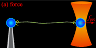
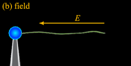
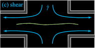
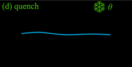
Figure 1: (color online) In the “force” scenario (a), a stretching force $f_{\mathrm{pre}}$ is suddenly removed at both ends. In the “field” setup (b), one end is held fixed and the electric field of strength $E$ (or homogeneous elongational flow of velocity $v$) is switched off, similar to the “shear” case (c) with a symmetric extensional shear flow of shear rate $\dot{\gamma}$. In the “quench” experiment (d), the temperature is suddenly increased by a large factor $\theta$ from an initially small value.

The paper is organized as follows. In the first section, we present results from Brownian dynamics simulations for each of the four different setups. The next section presents a qualitative discussion of the underlying theoretical model resulting in scaling laws for pertinent observables, which readily suggest intuitive explanations for the qualitative differences between the scenarios and their universal long-time asymptote. A detailed and somewhat technical derivation of these asymptotic scaling laws is contained in the third section, where we also analyze the effect of different boundary conditions. In the fourth section, we present a quantitative comparison between simulation results and theory. At the end of the paper, we discuss experimental implications including quantitative estimates of control parameters in typical realizations, the onset of the stretch–coil transition and the influence of hydrodynamic interactions.

I Simulation results

In the Brownian dynamics simulation, we employ the standard free-draining bead-spring algorithm for wormlike chains, were different environmental conditions during equilibration of the chains correspond to the four scenarios introduced above. The equations of motion for a chain of total length $L=Nb$ with $N+1$ beads of size $b$ and mobility $\mu$ are given by

$$\partial_{t}\bm{r}_{i}-\bm{v}_{i}=-\mu\bm{\nabla}_{i}U+\bm{\eta}_{i}(t),$$ (1)

where the potential $U=U_{\text{s}}+U_{\text{b}}+U_{\text{f}}$ contains a stretching part

$$U_{\text{s}}=\frac{k_{\mathrm{B}}T\gamma_{\text{s}}}{2b}\sum_{i}(\left|\bm{r}_{i+1}-\bm{r}_{i}\right|-b)^{2},$$ (2)

a bending part

$$U_{\text{b}}=\frac{k_{\mathrm{B}}T\ell_{\mathrm{p}}}{b}\sum_{i}(1-\bm{t}_{i+1}\cdot\bm{t}_{i}),$$ (3)

and an external potential $U_{\mathrm{f}}$. Here, $\ell_{\mathrm{p}}$ is the persistence length, $\gamma_{\text{s}}$ is the stretching elastic constant, and $\bm{t}_{i}=\frac{\bm{r}_{i}-\bm{r}_{i-1}}{\left|\bm{r}_{i}-\bm{r}_{i-1}\right|}$ is a normalized tangent vector. We use Gaussian noise with strength $\left\langle\bm{\eta}_{i}(t)\bm{\eta}_{j}(t^{\prime})\right\rangle=6\mu k_{\mathrm{B}}T\delta_{ij}\delta(t-t^{\prime})$. The time step is $10^{-5}\tau_{0}$, where $\tau_{0}=b^{2}/(k_{\mathrm{B}}T\mu)$ is the self-diffusion time of the beads. The chains are equilibrated along the $x$-axis symmetrically to the origin under the respective stretching mechanism. In the “force” case, $U_{\mathrm{f}}=-f_{\mathrm{pre}}(x_{N}-x_{0})$ and $\bm{v}_{i}=0$, while $U_{\mathrm{f}}=0$ and $\bm{v}_{i}=(v,0,0)^{T}$ for “field” setups. For “shear”, we take $\bm{v}_{i}=\dot{\gamma}\,(x_{i},-y_{i},-z_{i})^{T}$, and in order to prevent the polymer from diffusing out of the stagnation point, an additional harmonic potential $U_{\mathrm{f}}=\frac{1}{2}\dot{\gamma}\mu^{-1}x_{\mathrm{COM}}^{2}$ drives the center-of-mass coordinate $x_{\mathrm{COM}}$ back to the origin (cf. the feedback control system in Ref. schroeder-babcock-shaqfeh-chu:03 ). In these scenarios, we equilibrate for $10^{4}$ time steps, while initial conformations are generated directly using the equilibrium tangent correlations in the “quench” case. In all cases, $U_{\mathrm{f}}=0$ and $\bm{v}_{i}=0$ upon release. Ensemble averages were taken over 150 realizations

To characterize the relaxation dynamics, we concentrate on two observables. One is the time dependent change $\delta R_{\parallel}(t)=R_{\parallel}(0)-R_{\parallel}(t)$ in the ensemble average of the filament’s end-to-end distance $R_{\parallel}$, projected onto the initial longitudinal axis. Note that with this definition, $\delta R_{\parallel}$ is positive and increasing, while the actual end-to-end distance shrinks during relaxation. The second observable is the mean tension $\bar{f}_{\mathrm{b}}(t)$ in the filament, proportional to the bulk stress $\sigma(t)$ in a polymer solution. Fig. 2 shows simulation results for $\delta R_{\parallel}(t)$, measured from the projection on the initial longitudinal axis, and for $\bar{f}_{\mathrm{b}}(t)$ (proportional to the sum of the spring displacements from their equilibrium position). Parameters were chosen such that the initial extension is close to full stretching ($R_{\parallel}(0)\approx 0.97L$ in all cases). While the universal scaling for longer times is evident (the apparent systematic offset in the “field” case arises simply because there is only one free end), substantial differences between the scenarios for shorter times are clearly observable as well.

\psfrag{X1}{$\tau/\tau_{0}$}\psfrag{X2}{$\tau/\tau_{0}$}\psfrag{Y1}{$\delta R_{\parallel}(t)/L$}\psfrag{Y2}{$\bar{f}_{\mathrm{b}}(t)/(k_{\mathrm{B}}T/b)$}\includegraphics[angle={270},width=208.13574pt]{results-plot-notheory}

Figure 2: (color online) Quantitative results: change in projected length $\delta R_{\parallel}(t)$ and mean bulk tension $\bar{f}_{\mathrm{b}}(t)$ (inset) for computer simulations of a “force” (squares), “field” (triangles), “shear” (circles) and “quench” (diamonds) scenario, respectively. Simulation parameters were $L=200b$, $\ell_{\mathrm{p}}=40b$, $\gamma_{\text{s}}=6000/b$, $f_{\mathrm{pre}}=10\ k_{\mathrm{B}}T/b$, $v=0.18\ b/\tau_{0}$, $\dot{\gamma}=0.0046/\tau_{0}$ and $\theta=35.7$, such that $R_{\parallel}(0)\approx 0.97L$ in all cases.

II Qualitative theoretical results

From Fig. 2 it is obvious that the time evolution of $\delta R_{\parallel}(t)$ and $\bar{f}_{\mathrm{b}}(t)$ does not obey simple power law scaling. Simplifying approaches based on scaling arguments brochard:95 ; maier-seifert-raedler:02 , elastic dumbbell models ladoux-doyle:00 ; schroeder-shaqfeh-chu:04 , or quasi-equilibrium approximations brochard-buguin-degennes:99 ; crut-etal:07 have sometimes been used successfully for specific situations and parameter ranges. In contrast, we employ a systematic formalism hallatschek-frey-kroy:05 based on the wormlike chain model, which allows to generally account for the complex dynamics resulting from different environmental perturbations. Here, we first present qualitative results for all four scenarios in order to illustrate their differences, and discuss exact analytical and numerical results in the next section.

In the wormlike chain model saito-takahashi-yunoki:67 , semiflexible polymers are represented as inextensible smooth spacecurves $\bm{r}(s,t)$ of length $L$. Bending energy is proportional to the squared local curvature $(\partial_{s}^{2}\bm{r})^{2}$, such that in equilibrium, tangent orientations are correlated over the persistence length $\ell_{\mathrm{p}}=\kappa/k_{\mathrm{B}}T$, where $\kappa$ is the bending rigidity. The initially straight polymer is supposed to be equilibrated at times $t<0$ and released at $t=0$. After that, the longitudinal contraction is driven energetically uphill via the creation of contour undulations by entropic forces. Considering the conservation of contour length due to the (near) inextensibility of the backbone bonds, these transverse wrinkles are conveniently referred to in terms of their excess contour length, or stored length, with an associated line density $\varrho$. Mathematically, the inextensibility is enforced by the backbone tension $f$ which counteracts stretching, and the creation of stored length is accompanied by the relaxation of tension. The theory of Refs. hallatschek-frey-kroy:05 ; hallatschek-frey-kroy:07a relates the tension $f(s,t)$ to the stored length density $\varrho(s,t)$, based on the weakly-bending limit of small contour deviations from a straight line. In practice, this can easily be realized by choosing the control parameters $f_{\mathrm{pre}}$, $E$ or $v$, or $\dot{\gamma}$ sufficiently strong (as in typical experiments, see Table 3 below), or the quenching factor $\theta$ sufficiently large. It also justifies the free-draining approximation, where hydrodynamic effects are captured by anisotropic local friction coefficients $\zeta_{\perp,\parallel}$ (per length) for transverse/longitudinal friction, respectively doi-edwards:86 . However, ordinary perturbation theory is applicable only for late times $t\gg t_{\star}\simeq\zeta_{\parallel}L^{8}/(k_{\mathrm{B}}T\ell_{\mathrm{p}}^{5})$ hallatschek-frey-kroy:05 , because to lowest order it allows only a linear spatial dependence of $\varrho$ and $f$ and neglects longitudinal friction forces seifert-wintz-nelson:96 . Further, except for quite stiff filaments with $\ell_{\mathrm{p}}\gtrsim L$, the time $t_{\star}$ is usually larger than the filament’s longest relaxation time $t_{\mathrm{R}}\simeq\zeta_{\parallel}\ell_{\mathrm{p}}L^{2}/k_{\mathrm{B}}T$ hallatschek-frey-kroy:07b , which within our approximations is given by the Rouse time of a polymer with Kuhn length $2\ell_{\mathrm{p}}$. Nevertheless, with an improved formalism hallatschek-frey-kroy:05 ; hallatschek-frey-kroy:07a including nontrivial spatial variations in $f$ and $\varrho$, the conformational relaxation at times $t\ll t_{\mathrm{R}}$ can be analyzed even for quite flexible polymers. This leads to the remarkable insight that weakly-bending polymers constitute self-averaging systems: the small stochastic fluctuations average out along the contour and the coarse-grained tension dynamics follows from the deterministic relation

$$\partial_{s}^{2}\bar{f}=-\zeta_{\parallel}\partial_{t}\left\langle\bar{\varrho}\right\rangle,$$ (4)

where the overbar denotes a (local) spatial average that produces effectively an ensemble average (denoted by $\left\langle\ .\ \right\rangle$) hallatschek-frey-kroy:07a . Driven by tension gradients, stored length propagates subdiffusively from the filament’s ends into the bulk—limited to boundary layers of size $\ell_{\parallel}(t)$ by longitudinal solvent friction. In more intuitive terms, the filament starts to “coil up” first at the boundaries, and only later in the bulk, see also Fig. 3.

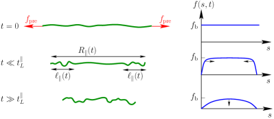
Figure 3: (Color online) Schematic representation of conformational (left) and tension relaxation (right) in a “force” setup. For $t=0$, the filament is equilibrated under the force $f_{\mathrm{pre}}$. As the ends are released, the contour coils up in two growing boundary layers of size $\ell_{\parallel}(t)$ where the tension relaxes. At $t=t_{L}^{\parallel}$, the dynamics crosses over from the propagation to the relaxation regime and the tension relaxes to zero.

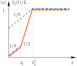
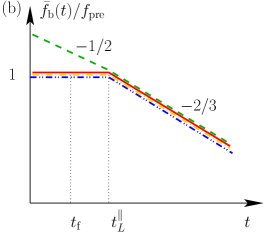
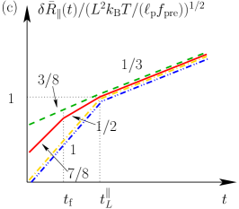
Figure 4: (color online) Qualitative results. Asymptotic scaling laws for the boundary layer size $\ell_{\mathrm{p}}(t)$ (a), the mean bulk tension $\bar{f}_{\mathrm{b}}(t)$ or the bulk stress (b), and for the change in projected length $\delta\bar{R}_{\parallel}(t)$ (c) in “force” (solid), “field” (dot-dashed), “shear” (dot-dot-dashed), or “quench” (dashed) setups, respectively.

In general, $\left\langle\bar{\varrho}\right\rangle$ is a nonlinear functional of $\bar{f}$, see Eq. (10) below for a detailed expression. Exact analytical results for the boundary layer size $\ell_{\parallel}(t)$, the bulk tension $\bar{f}_{\mathrm{b}}(t)$, and the change in projected length $\delta R_{\parallel}(t)$ will be obtained as leading-order results of a systematic asymptotic expansion of Eq. (4) in the next section. However, the scaling of the dominant part $\delta\bar{R}_{\parallel}(t)$ of $\delta R_{\parallel}(t)$, which is independent of boundary conditions and an effectively deterministic quantity, can be found from a simple dimensional argument: the change in end-to-end distance equals the amount of stored length $\varrho\ell_{\parallel}$ that has been created in the boundary layer. On the scaling level, Eq. (4) reads $\bar{f}_{\mathrm{b}}/\ell_{\parallel}^{2}\simeq\zeta_{\parallel}\varrho/t$, and we obtain

$$\delta\bar{R}_{\parallel}\simeq\frac{t\bar{f}_{\mathrm{b}}}{\zeta_{\parallel}\ell_{\parallel}}.$$ (5)

Note that the change $\delta R_{G}(t)$ in the gyration tensor’s largest eigenvalue, which is frequently identified with $\delta R_{\parallel}$ nam-lee:07 ; dimitrakopoulos:04 , obeys a different scaling law $\delta R_{G}\simeq t\bar{f}_{\mathrm{b}}/(\zeta_{\parallel}L)$ for short times $t\ll t_{L}^{\parallel}$ hallatschek-frey-kroy:04 . Additional subdominant contributions to $\delta R_{\parallel}(t)$ from end fluctuations will be analyzed in section III.

Fig. 4 summarizes the scaling results of section III for $\ell_{\parallel}(t)$, $\bar{f}_{\mathrm{b}}(t)$, and $\bar{\delta}R_{\parallel}(t)$ in various intermediate asymptotic regimes, which are separated by different crossover times that have been matched by an appropriate choice of the respective control parameters for better comparison. Clearly, the time $t_{L}^{\parallel}=\zeta_{\parallel}L^{2}[k_{\mathrm{B}}T/(\ell_{\mathrm{p}}f_{\mathrm{pre}}^{3})]^{1/2}$ is of key importance since it separates scenario-specific and universal relaxation. To understand the origin of the differences for times $t\ll t_{L}^{\parallel}$, we will consider the different scenarios separately before we address the universal regime $t\gg t_{L}^{\parallel}$.

“Force” setup.

After the stretching force has been shut off, the polymer starts to build up contour undulations driven by thermal noise. These transverse undulations appear first in growing boundary layers of size $\ell_{\parallel}(t)\ll L$ near the ends: assuming an inextensible backbone, the immediate creation of undulations in the bulk would require the ends to be pulled inwards against longitudinal solvent friction with a force exceeding the actual backbone tension. This phenomenon of tension propagation ends after a time $t_{L}^{\parallel}$, defined via $\ell_{\parallel}(t_{L}^{\parallel})=L$, where the boundary layers extend over the whole polymer length, see Fig. 3. A more detailed analysis hallatschek-frey-kroy:05 shows that the longitudinal relaxation depends on whether the internal tension (initially equal to the stretching force $f_{\mathrm{pre}}$) represents a relevant perturbation to the transverse conformational dynamics. The latter undergoes a dynamic crossover from a bending-dominated regime with $\ell_{\parallel}\propto t^{1/8}$ everaers-juelicher-ajdari-maggs:99 for the shortest times $t\ll t_{\mathrm{f}}$ to a tension-driven regime with $\ell_{\parallel}\propto t^{1/2}$ brochard-buguin-degennes:99 for longer times $t\gg t_{\mathrm{f}}$, where the dynamics becomes inherently nonlinear. Here, $t_{\mathrm{f}}=\zeta_{\perp}k_{\mathrm{B}}T\ell_{\mathrm{p}}/f_{\mathrm{pre}}^{2}$ is a crossover time that obeys $t_{\mathrm{f}}\ll t_{L}^{\parallel}$ for reasonably large prestress $f_{\mathrm{pre}}$ (see Table 3 below).

“Field” and “shear” setup.

Similarly, one can define a force equivalent in “field” or “shear” experiments and corresponding expressions for $t_{\mathrm{f}}$ and $t_{L}^{\parallel}$: the hydrodynamic equivalent of $f_{\mathrm{pre}}$ is simply the total Stokes friction $\zeta_{\parallel}vL$ in a homogeneous flow, and $\zeta_{\parallel}\dot{\gamma}L^{2}$ is the longitudinal friction in an extensional shear flow. Flow conditions may straightforwardly be recast into the equivalent language of external (e.g., electrical) fields. However, complicated counterion effects long-viovy-ajdari:96a ; stigter-bustamante:98 ; heuvel-graaff-lemay-dekker:07 prevent the quantitative prediction of the equivalent electrophoretic field strength $E$ for typical experimental realizations. Although field-type perturbations induce dynamic crossovers at $t_{\mathrm{f}}$ similar to the “force” case, the change $\delta R_{\parallel}(t)$ in projected length increases always linearly with time. This can be understood by a simple change in perspective: the polymer’s ends are pulled inwards by an approximately constant bulk tension, i.e., with roughly constant velocity. This corresponds in the frame of reference of the ends to an external flow field. The resulting friction forces are properly balanced and the initial polymer conformations are already equilibrated under such a flow field in “field” and “shear” setups, in contrast to the “force” scenario. Tension propagation is therefore not a dominant effect in the former (Eq. (5) applies with $\ell_{\parallel}\equiv L$ because of the large-scale spatial variation of the tension), and the constant drag gives $\delta\bar{R}_{\parallel}\propto t$.

“Quench” setup.

Here, finally, there is no external force scale and therefore no dynamic crossover ($\ell_{\parallel}\propto t^{1/8}$ for $t\ll t_{L}^{\parallel}$), although the parameter combination $k_{\mathrm{B}}T\ell_{\mathrm{p}}^{3}\theta^{4}/L^{4}$ plays the role of $f_{\mathrm{pre}}$ in the crossover time $t_{L}^{\parallel}$. The tension in a quenched filament is produced solely by the suddenly increased thermal noise from the environment (if the external temperature increases), or by the suddenly higher “sensitivity” to this noise (if the quenching is achieved by a sudden drop in bending rigidity). Hence, its magnitude depends on the “mismatch” between the current conformation and an equilibrium conformation corresponding to the current environment. Therefore, the quenched filament can relax tension even in the bulk, by reshuffling stored length between long and short wavelength modes in a way similar to the mechanical stress relaxation in buckled rods hallatschek-frey-kroy:04 , while the bulk tension stays constant for $t\ll t_{L}^{\parallel}$ in the other setups.

Universal regime.

At long times $t\gg t_{L}^{\parallel}$, when the tension has propagated through the filament, the dynamics enters the universal regime of homogeneous tension relaxation hallatschek-frey-kroy:05 . Contrary to previous assumptions bohbot_raviv-etal:04 , longitudinal friction may not generally be neglected, but dominates the dynamics in this regime. The tension has a nontrivial spatial dependence, but it can for asymptotically large forces be treated as quasi-statically equilibrated brochard-buguin-degennes:99 ; hallatschek-frey-kroy:05 . The characteristic universality of the long-time relaxation is then simply a consequence of the right hand side of Eq. (4) being independent of initial conditions: $\bar{\varrho}\approx[k_{\mathrm{B}}T/(4\ell_{\mathrm{p}}\bar{f})]^{1/2}$, where we have used the (static) force-extension relation for wormlike chains marko-siggia:95 . This asymptote readily implies by Eq. (4) the scaling $\bar{f}\propto t^{-2/3}$ and by Eq. (5) the characteristic $t^{1/3}$-growth of $\delta\bar{R}_{\parallel}(t)$, which has indeed been observed in experiments schroeder-shaqfeh-chu:04 . As an aside, we note that $t_{\star}<t_{\mathrm{R}}$ for stiff polymers with $L\lesssim\ell_{\mathrm{p}}$; the adjoining regime of algebraic relaxation for times $t_{\star}\ll t$ shows a $t^{1/4}$-scaling in $\delta\bar{R}_{\parallel}(t)$ granek:97 ; hallatschek-frey-kroy:05 .

Let us finally comment on the joint limiting scenario: the exactly straight initial conformation (as in Ref. dimitrakopoulos:04 ). Not only it is quite artificial from a theoretical and experimental perspective, it also appears to be ambiguous, since we could let $f_{\mathrm{pre}}\to\infty$ in one of the scenarios involving external forces as well as $\theta\to\infty$ for the “quench” case. Although $t_{L}^{\parallel}\to 0$ in both cases, so that only the universal regime survives and the ambiguity is limited to $t=0$, it gives rise to observable effects as soon as one takes into account some microstructure corrections important for real experimental systems and simulation models obermayer:unpub .

After this qualitative discussion of the relaxation dynamics, we will now present a systematic derivation and analysis of Eq. (4), resulting in exact growth laws in various intermediate asymptotic regimes for the observables introduced above. While Ref. hallatschek-frey-kroy:07b only covered the “force” case, we now obtain results for the other scenarios as well, and include a quantitative analysis of different boundary conditions.

III Quantitative theoretical results

Starting point for our calculations is the wormlike-chain Hamiltonian

$$\mathcal{H}=\frac{1}{2}\int_{0}^{L}\!\mathrm{d}s\left[\kappa\bm{r}^{\prime\prime 2}+f\bm{r}^{\prime 2}\right],$$ (6)

where the backbone tension $f(s,t)$, a Lagrange multiplier function goldstein-langer:95 , takes care of the local inextensibility constraint $\bm{r}^{\prime}(s)^{2}=1$. The equations of motion for the contour result from balancing elastic forces $-\partial\mathcal{H}/\partial\bm{r}$ with stochastic noise $\bm{\xi}$ and anisotropic viscous local friction forces $\bm{\zeta}[\partial_{t}\bm{r}-\bm{u}]$ with friction matrix $\bm{\zeta}=[\zeta_{\perp}\bm{r}^{\prime}\bm{r}^{\prime}+\zeta_{\parallel}(1-\bm{r}^{\prime}\bm{r}^{\prime})]$ and a velocity field $\bm{u}$ of the solvent. The friction coefficients (per length) are $\zeta_{\parallel}=\hat{\zeta}\zeta_{\perp}$ with $\hat{\zeta}\approx 1/2$ and $\zeta_{\perp}\approx 4\pi\eta/\ln(L/a)$ doi-edwards:86 , where $a$ is the backbone thickness. In all of this section, we set $\zeta_{\perp}=\kappa\equiv 1$ for simplicity. This makes time a length⁴ and the tension a length^-2. Note that $\kappa=k_{\mathrm{B}}T\ell_{\mathrm{p}}$ is kept constant in the “quench” scenario. Our approach exploits the weakly-bending limit. Parameterizing the contour $\bm{r}=(\bm{r}_{\bot},s-r_{\parallel})^{T}$ in terms of small transverse and longitudinal displacements from the straight ground state, this means that $\bm{r}_{\bot}^{\prime 2}=\mathcal{O}(\varepsilon)\ll 1$, with $\varepsilon=f_{\mathrm{pre}}^{-1/2}/\ell_{\mathrm{p}}$ for “force” setups (and $f_{\mathrm{pre}}$ replaced by its equivalents in “field” or “shear” scenarios) and $\varepsilon=L/(\theta\ell_{\mathrm{p}})$ for “quench” setups, respectively. Up to order $\varepsilon$, the equations of motion for the contour in absence of external forces and for $\bm{u}=0$ read:

$$\partial_{t}\bm{r}_{\bot} =-\bm{r}_{\bot}^{\prime\prime\prime\prime}+(f\bm{r}_{\bot}^{\prime})^{\prime}+\bm{\xi}_{\perp}$$ (7a)

$$\hat{\zeta}\partial_{t}r_{\parallel}+(1-\hat{\zeta})\bm{r}_{\bot}^{\prime}\partial_{t}\bm{r}_{\bot} =-r_{\parallel}^{\prime\prime\prime\prime}-f^{\prime}+(fr_{\parallel}^{\prime})^{\prime}+\xi_{\parallel}$$ (7b)

Because in the weakly-bending limit the transverse contour fluctuations are correlated on much shorter length scales than the longitudinal (= tension) dynamics, we can formally introduce “fast” and “slow” arclength coordinates for the small-scale transverse and large-scale longitudinal dynamics, respectively hallatschek-frey-kroy:07a . Taking a local (with respect to $\ell_{\parallel}$) spatial average over the small-scale fluctuations (denoted by an overbar) leads to closed equations:

$$\partial_{t}\bm{r}_{\bot} =-\bm{r}_{\bot}^{\prime\prime\prime\prime}+\bar{f}\bm{r}_{\bot}^{\prime\prime}+\bm{\xi}_{\perp}$$ (8a)

$$\partial_{s}^{2}\bar{f} =-\hat{\zeta}\partial_{t}\left\langle\bar{\varrho}\right\rangle.$$ (8b)

The longitudinal part Eq. (8b), where $\varrho=\tfrac{1}{2}\bm{r}_{\bot}^{\prime 2}$ is the stored length density, follows from the self-averaging property of weakly-bending polymers: the spatial coarse-graining effectively generates an ensemble average. The transverse part Eq. (8a) contains a locally constant tension $\bar{f}$ (its slow arclength dependence obtained through Eq. (8b) is adiabatically inherited), and can be solved in terms of appropriate eigenmodes $w_{q}(s)$ with eigenvalue $-q^{2}(q^{2}+f(t))$ via the response function

$$\chi_{\perp}(q;t,t^{\prime})=\mathrm{e}^{-2q^{2}[q^{2}(t-t^{\prime})+\int_{t^{\prime}}^{t}\!\mathrm{d}\tau\bar{f}(\tau)]},$$ (9)

Using the noise correlation $\left\langle\bm{\xi}_{\perp}(k,t)\bm{\xi}_{\perp}(q,t^{\prime})\right\rangle=4\ell_{\mathrm{p}}^{-1}\delta_{k,q}\delta(t-t^{\prime})$, we evaluate the expectation value $\left\langle\tfrac{1}{2}\bm{r}_{\bot}^{\prime 2}\right\rangle$. The different preparation mechanisms discussed in the main text constrain the polymer only for $t<0$. Including the initial conditions $\bar{f}(s,t<0)=\bar{f}_{0}(s)$ and $\ell_{\mathrm{p}}(t>0)\equiv\ell_{\mathrm{p}}=\ell_{\mathrm{p}}(t<0)/\theta$ gives for the stored length density

$$\left\langle\varrho\right\rangle=\frac{1}{\ell_{\mathrm{p}}}\sum_{q}\Bigg{[}\frac{\chi_{\perp}^{2}(q;t,0)}{q^{2}\theta(q^{2}+\bar{f}_{0}(s))}\\ +2\int_{0}^{t}\!\mathrm{d}t^{\prime}\,\chi_{\perp}^{2}(q;t,t^{\prime})\Bigg{]}w_{q}^{\prime 2}(s)$$ (10)

As only the spatially averaged stored length density $\left\langle\bar{\varrho}\right\rangle$ enters Eq. (8b), we decompose $w_{q}^{\prime 2}(s)$ into a spatially constant and a fluctuating part $c_{q}(s)$ (the latter will average out upon coarse-graining):

$$w_{q}^{\prime 2}(s)=\frac{q^{2}}{L}\left[1+c_{q}(s)\right].$$ (11)

Taking the continuum limit $L\to\infty$ and integrating Eq. (8b) over time, we find that the integrated tension $\bar{F}(s,t)=\int_{0}^{t}\!\mathrm{d}t^{\prime}\bar{f}(s,t^{\prime})$ obeys the partial integro-differential equation

$$\partial_{s}^{2}\bar{F}(s,t)=\hat{\zeta}\int_{0}^{\infty}\!\frac{\mathrm{d}q}{\pi\ell_{\mathrm{p}}}\Bigg{[}\frac{1-\chi_{\perp}^{2}(q;t,0)}{\theta(q^{2}+\bar{f}_{0}(s))}\\ -2q^{2}\int_{0}^{t}\!\mathrm{d}t^{\prime}\chi_{\perp}^{2}(q;t,t^{\prime})\Bigg{]}.$$ (12)

From solutions to this equation in different intermediate asymptotic regimes presented in the next subsection, we will then infer growth laws for the two observables.

III.1 Asymptotic results for the tension

III.1.1 “Force” setup

This scenario with $\theta=1$ and the initial and boundary conditions

$$\begin{split}\bar{f}(s,t<0)=f_{\mathrm{pre}}\quad\text{ and }\\ \bar{f}(0,t>0)=0,\quad\bar{f}(L,t>0)=0,\end{split}$$ (13)

is identical to the “release”-scenario which was thoroughly analysed in Ref. hallatschek-frey-kroy:07b . We will briefly sketch this analysis in order to motivate its application to the other setups. From the response function Eq. (9), we get the asymptotic scaling for the wave number $Q$ of the mode that relaxes at time $t$:

$$Q\simeq\begin{cases}t^{-1/4},&\quad\text{if }\bar{F}^{2}/t\ll 1\quad\text{(``linear'')}\\ \bar{F}^{-1/2},&\quad\text{if }\bar{F}^{2}/t\gg 1\quad\text{(``nonlinear'')}\end{cases}$$ (14)

Examining Eq. (8a), one infers that in the first case the tension contribution $Q^{2}\bar{F}$ is small compared to the bending contribution $Q^{4}t$ and can be treated as perturbation on the linear level. Since the magnitude of the tension is determined by the prestretching force, $\bar{F}\simeq f_{\mathrm{pre}}t$, this asymptote, called “linear regime”, can also be formulated as $t\ll t_{\mathrm{f}}$ with $t_{\mathrm{f}}=f_{\mathrm{pre}}^{-2}$. In the second case $t\gg t_{\mathrm{f}}$, the bending contributions are subdominant which leads to different “nonlinear regimes”.

Linear propagation ($t\ll t_{\mathrm{f}}$).

We perform an expansion obermayer-hallatschek-frey-kroy:07 of the right hand side of Eq. (12) with respect to the integrated tension $\bar{F}$ and to the force $f_{\mathrm{pre}}$:

$$\partial_{s}^{2}\bar{F}(s,t)\approx\hat{\zeta}\int_{0}^{\infty}\!\frac{\mathrm{d}q}{\pi\ell_{\mathrm{p}}}\Bigg{[}-\frac{f_{\mathrm{pre}}}{q^{4}}\left(1-\mathrm{e}^{-2q^{4}t}\right)\\ +2\bar{F}(s,t)-4q^{4}\int_{0}^{t}\!\mathrm{d}t^{\prime}\,\bar{F}(s,t^{\prime})\mathrm{e}^{-2q^{4}(t-t^{\prime})}\Bigg{]}.$$ (15)

Using the Laplace transform $\tilde{F}(s,z)=\mathcal{L}\{\bar{F}(s,t)\}$, this reads

$$\partial_{s}^{2}\tilde{F}(s,z)=\hat{\zeta}\int_{0}^{\infty}\!\frac{\mathrm{d}q}{\pi\ell_{\mathrm{p}}}\left[-\frac{2f_{\mathrm{pre}}}{z(z+2q^{4})}+\tilde{F}(s,z)\frac{2z}{z+2q^{4}}\right],$$ (16)

which, after performing the $q$-integral, reduces to:

$$\lambda^{2}\,\partial_{s}^{2}\tilde{F}=\tilde{F}-\frac{f_{\mathrm{pre}}}{z^{2}}.$$ (17)

Here, $\lambda(z)=2^{3/8}(\ell_{\mathrm{p}}/\hat{\zeta})^{1/2}z^{-1/8}$ is a dynamic length scale denoting the size of spatial variations in $\tilde{F}(s,z)$. If $L\gg\lambda$, the solution to Eq. (17) varies only close to the boundaries, as it is characteristic for the propagation regime. Near $s=0$ (and correspondingly near $s=L$), it simplifies to

$$\tilde{F}(s,z)\approx\frac{f_{\mathrm{pre}}}{z^{2}}\left[1-\mathrm{e}^{-s/\lambda}\right],$$ (18)

which can be backtransformed hallatschek-frey-kroy:07b to

$$\bar{F}(s,t)=f_{\mathrm{pre}}\,t\left[1-\phi(s/\ell_{\parallel}(t))\right],$$ (19)

where $\phi(\xi)\approx\exp[-2^{-3/8}\xi/\mathrm{\Gamma}\left(15/8\right)]$ is a scaling function that depends only on the ratio $\xi=s/\ell_{\parallel}(t)$. The length scale $\lambda$ is directly related to the boundary layer size $\ell_{\parallel}(t)=(\ell_{\mathrm{p}}/\hat{\zeta})^{1/2}t^{1/8}$ everaers-juelicher-ajdari-maggs:99 ; hallatschek-frey-kroy:05 ; hallatschek-frey-kroy:07b , and the requirement $L\gg\lambda$ translates into $t\ll t_{L}^{\parallel}$.

Nonlinear propagation ($t_{\mathrm{f}}\ll t\ll t_{L}^{\parallel}$).

In the nonlinear regime, the $Q^{4}t$ bending contributions are small compared to the tension terms $Q^{2}\bar{F}$ if $\bar{F}^{2}/t\gg 1$. This results in $\chi_{\perp}(q;t,t^{\prime})$ being finite only near $t^{\prime}\approx t$, see Eq. (9). We can therefore linearize $\bar{F}(s,t)-\bar{F}(s,t^{\prime})\approx[\partial_{t}\bar{F}(s,t)](t-t^{\prime})$ in the exponent. The $t^{\prime}$-integral in the second term of Eq. (12) is readily performed hallatschek-frey-kroy:07b :

$$\partial_{s}^{2}\bar{F} \approx\hat{\zeta}\int_{0}^{\infty}\!\frac{\mathrm{d}q}{\pi\ell_{\mathrm{p}}}\left[\frac{1-\chi_{\perp}^{2}(q;t,0)}{q^{2}+f_{\mathrm{pre}}}-\frac{1-\chi_{\perp}^{2}(q;t,0)}{q^{2}+\partial_{t}\bar{F}}\right]$$

$$\approx\hat{\zeta}\int_{0}^{\infty}\!\frac{\mathrm{d}q}{\pi\ell_{\mathrm{p}}}\left[\frac{1}{q^{2}+f_{\mathrm{pre}}}-\frac{1}{q^{2}+\partial_{t}\bar{F}}\right]$$

$$=\frac{\hat{\zeta}}{2\ell_{\mathrm{p}}}\left[f_{\mathrm{pre}}^{-1/2}-(\partial_{t}\bar{F})^{-1/2}\right].$$ (20)

In the second line, we let $\chi_{\perp}\to 0$ because $\bar{F}^{2}/t\gg 1$. This indicates the underlying “quasi-static” approximation: the relevant modes have already decayed and the tension is quasi-statically equilibrated. Taking a time derivative gives brochard-buguin-degennes:99 ; hallatschek-frey-kroy:07b

$$\partial_{s}^{2}\bar{f}=\frac{\hat{\zeta}\partial_{t}\bar{f}}{4\ell_{\mathrm{p}}\bar{f}^{3/2}}.$$ (21)

Inspired by the result Eq. (19), we expect a scaling form $\bar{f}(s,t)=f_{\mathrm{pre}}\varphi(\xi)$ with $\xi=s/\ell_{\parallel}(t)$ for the tension. Inserting it into Eq. (21) gives $\ell_{\parallel}(t)=(\ell_{\mathrm{p}}/\hat{\zeta})^{1/2}f_{\mathrm{pre}}^{3/4}t^{1/2}$ brochard-buguin-degennes:99 ; hallatschek-frey-kroy:05 and

$$\partial_{\xi}^{2}\varphi=-\frac{1}{8}\xi\varphi^{-3/2}\partial_{\xi}\varphi,$$ (22)

with the boundary conditions $\varphi(0)=0$ and $\partial_{\xi}\varphi(\xi\to\infty)=0$, i.e., we neglect the presence of the second end, where the situation is correspondingly, and assume just a flat profile in the bulk. Numerical solutions to this equation have been shown in Refs. brochard-buguin-degennes:99 ; hallatschek-frey-kroy:07b and give $\varphi(\xi\to\infty)=1$ as expected and $\varphi^{\prime}(0)\approx 0.62$. The propagation regime ends at $t_{L}^{\parallel}=L^{2}f_{\mathrm{pre}}^{-3/2}/\ell_{\mathrm{p}}$.

Homogeneous relaxation ($t_{L}^{\parallel}\ll t\ll t_{\mathrm{R}}$).

After the tension has propagated through the filament, it is no longer constant but expected to decay. But as long as $\bar{F}^{2}/t\gg 1$ still holds, we can use Eq. (21). Hence, we try the separation ansatz $\bar{f}(s,t)=g(t)h(\xi)$ with $\xi=s/L$, which gives hallatschek-frey-kroy:07b

$$g(t)=\left(\frac{\hat{\zeta}L^{2}}{\ell_{\mathrm{p}}t}\right)^{2/3},$$ (23)

and

$$h^{\prime\prime}=-\tfrac{1}{6}h^{-1/2}\quad\text{with }h(0)=h(1)=0.$$ (24)

The almost parabolic profile $h(\xi)$ is characterized by hallatschek-frey-kroy:07b

$$h^{\prime}(0)=12^{-1/3},\quad h(1/2)=\left(\tfrac{3}{128}\right)^{2/3}.$$ (25)

Using Eq. (23), we find that the condition $\bar{F}^{2}/t\gg 1$ is violated for $t\gtrsim t_{\star}=L^{8}/\ell_{\mathrm{p}}^{4}$, which is already larger than $t_{\mathrm{R}}$ if $\ell_{\mathrm{p}}\lesssim L$. Hence, this regime lasts until the weakly-bending approximation breaks down near the ends due to the onset of the stretch–coil transition.

III.1.2 “Field” setup

For hydrodynamic and/or electrophoretic forces, we find from the longitudinal equation of motion Eq. (7b) a corresponding non-uniform initial tension profile $\bar{f}(s,t<0)=g(L-s)$ with $g=\hat{\zeta}v$ for flows or $g\propto E$ for an electric field, where the generally unknown prefactor is some combination of electrophoretic and hydrodynamic mobility. This linearly decreasing prestress would in principle lead to an additional term $\bar{f}^{\prime}\bm{r}_{\bot}^{\prime}$ in Eq. (8a), and the corresponding eigenfunctions would be very complicated. However, because large scale tension variations are irrelevant for the short wavelength transverse dynamics, we can ignore this term by consistently exploiting the scale separation which allowed the derivation of Eq. (8), and use Eq. (12) with the initial linear profile $\bar{f}_{0}(s)=g(L-s)$. The polymer is supposed to be grafted at $s=0$ and to have a free end at $s=L$, i.e., the boundary conditions are

$$\bar{f}^{\prime}(0,t>0)=0\quad\text{and}\quad\bar{f}(L,t>0)=0.$$ (26)

Identifying the force equivalent $f_{\mathrm{pre}}^{*}=gL$, we expect a linear regime for $t\ll t_{\mathrm{f}}$ with $t_{\mathrm{f}}=f_{\mathrm{pre}}^{*-2}$ and a nonlinear regime for $t\gg t_{\mathrm{f}}$, governed by the respective asymptotic differential equations from the “force” case.

Linear propagation ($t\ll t_{\mathrm{f}}$).

Linearizing Eq. (12) in $\bar{F}$ and $\bar{f}_{0}(s)$ and performing a Laplace transform as in Eqs. (15–17), we arrive at the solution

$$\bar{F}(s,t)=gt(L-s)-g\ell_{\parallel}(t)t\phi(s/\ell_{\parallel}(t)),$$ (27)

with $\ell_{\parallel}(t)=(\ell_{\mathrm{p}}/\hat{\zeta})^{1/2}t^{1/8}$ and $\phi(\xi)\approx\tfrac{2^{3/8}\exp[-\frac{\mathrm{\Gamma}\left(17/8\right)}{2^{3/8}}\xi]}{\mathrm{\Gamma}\left(17/8\right)}$. We find a boundary layer at the fixed end where the tension relaxes from its initial value $gL$ only by the small amount $g\ell_{\parallel}$. Near the free end, at $s=L$, we have $F(L,t)=0$ and $F^{\prime}(L,t)=-gt$ without any algebraic correction terms. Hence, because the tension at the free end is already very small and the contour does not further coil up, there are no boundary layer effects which would give relevant deviations from the linear drift towards the grafted end, in contrast to what has been found in Ref. maier-seifert-raedler:02 .

Nonlinear propagation ($t_{\mathrm{f}}\ll t\ll t_{L}^{\parallel}$).

The assumption $F^{2}/t\gg 1$ leads again to Eq. (21) except for very small regions near the free end where $\bar{f}_{0}(s)$ in the denominator of the first term of Eq. (12) is almost zero. Corresponding to the linear case Eq. (27), we assume that the tension deviates only near the fixed end from its initial value $\bar{f}_{0}(s)$. Hence, we insert $\bar{f}(s,t)=\bar{f}_{0}(s)-g\ell_{\parallel}(t)\varphi(\xi)$ with $\xi=s/\ell_{\parallel}(t)$ and $\ell_{\parallel}(t)=(\ell_{\mathrm{p}}/\hat{\zeta})^{1/2}(gL)^{3/4}t^{1/2}$ into Eq. (21), and expand about $\bar{f}_{0}(s\ll L)$:

$$\partial_{\xi}^{2}\varphi(\xi)\approx\frac{1}{8}\left[\varphi(\xi)-\xi\partial_{\xi}\varphi(\xi)\right]$$ (28)

with $\varphi^{\prime}(0)=-1$ and $\varphi(\xi\to\infty)=0$. The solution can be given in terms of the complementary error function:

$$\varphi(\xi)=\frac{4}{\sqrt{\pi}}\mathrm{e}^{-\xi^{2}/16}-\xi\operatorname{erfc}(\xi/4).$$ (29)

The propagation regime ends at $t_{L}^{\parallel}=L^{2}/(\ell_{\mathrm{p}}(gL)^{3/2})$.

Homogeneous relaxation ($t_{L}^{\parallel}\ll t\ll t_{\mathrm{R}}$).

The separation ansatz $\bar{f}(s,t)=g(t)h(\xi)$ with $\xi=s/L$ in Eq. (21) gives $g(t)=(\hat{\zeta}L^{2}/(\ell_{\mathrm{p}}t))^{2/3}$ as in Eq. (23) and the spatial function $h$ solves

$$h^{\prime\prime}=-\tfrac{1}{6}h^{-1/2}\quad\text{with }h^{\prime}(0)=0,\quad h(1)=0.$$ (30)

We find the following characteristics

$$h(0)=(\tfrac{3}{32})^{2/3},\quad h^{\prime}(1)=6^{-1/3}.$$ (31)

The condition $\bar{F}^{2}/t\gg 1$ holds until $t=t_{\mathrm{R}}$.

III.1.3 “Shear” setup

In this scenario, the equations of motion $\bm{\zeta}[\partial_{t}\bm{r}-\bm{u}]=-\delta\mathcal{H}/\delta\bm{r}+\bm{\xi}$ are modified in the presence of an extensional shear flow field $\bm{u}=\dot{\gamma}(-\bm{r}_{\bot},s-r_{\parallel}-L/2)^{T}$, where $\dot{\gamma}$ is the shear rate. To lowest order in $\varepsilon$, and in the stationary state, we obtain from Eq. (7b)

$$-\hat{\zeta}\dot{\gamma}\left(s-\tfrac{L}{2}\right)=\bar{f}^{\prime}.$$ (32)

As before, we treat this non-uniform tension profile only as large-scale variation and use Eq. (12) with the initial and boundary conditions

$$\begin{split}\bar{f}(s,t<0)=\tfrac{1}{2}\hat{\zeta}\dot{\gamma}s\,(L-s)\text{ and}\\ \bar{f}(0,t>0)=\bar{f}(L,t>0)=0.\end{split}$$ (33)

As in the “field” case, the time $t_{\mathrm{f}}=f_{\mathrm{pre}}^{*-2}$ with the force equivalent $f_{\mathrm{pre}}^{*}=\hat{\zeta}\dot{\gamma}L^{2}$ denotes the linear–nonlinear crossover.

Linear propagation ($t\ll t_{\mathrm{f}}$).

Here the solution to Eq. (17) reads

$$\bar{F}(s,t)=\tfrac{1}{2}\hat{\zeta}\dot{\gamma}ts(L-s)-\frac{2^{3/4}\hat{\zeta}\dot{\gamma}\ell_{\parallel}^{2}t}{\mathrm{\Gamma}\left(9/4\right)}\left[1-\phi(s/\ell_{\parallel}(t))\right],$$ (34)

with $\ell_{\parallel}=(\ell_{\mathrm{p}}/\hat{\zeta})^{1/2}t^{1/8}$ as before and $\phi(\xi)\approx\exp[-2^{-3/8}\mathrm{\Gamma}\left(9/4\right)\xi/\mathrm{\Gamma}\left(17/8\right)]$. We find two small boundary layers at the ends where the tension is slightly smaller than initially.

Nonlinear regime ($t_{\mathrm{f}}\ll t\ll t_{L}^{\parallel}$).

The nonlinear regime $t_{\mathrm{f}}\ll t\ll t_{L}^{\parallel}$ for the “shear” setup is quite peculiar: if we try (similar to the “force” and “field” case) a scaling ansatz $\bar{f}(s,t)=\frac{1}{2}\hat{\zeta}\dot{\gamma}[s(L-s)+L\ell_{\parallel}(t)\varphi(s/\ell_{\parallel}(t))]$ or similarly, we get $\ell_{\parallel}(t)\sim t^{2}$. This unusual result could be explained by the fact that the “prestress” $\bar{f}(s,t<0)\approx\frac{1}{2}\hat{\zeta}\dot{\gamma}sL$, which is responsible for the scaling of $\ell_{\parallel}$ in this regime obermayer-hallatschek-frey-kroy:07 , grows linearly with the distance from the ends. However, we dot not get any physically meaningful differential equation for $\varphi$ under the boundary conditions Eq. (33). We conclude that there is no propagation and no observable boundary layers. Looking for a solution spanning the whole arclength interval from $0$ to $L$ instead, we insert into Eq. (21) an expansion of the form

$$\bar{f}(s,t)=\tfrac{1}{2}\hat{\zeta}\dot{\gamma}L^{2}\left[\varphi_{0}(\xi)+\frac{t}{t_{L}^{\parallel}}\varphi_{1}(\xi)+\mathcal{O}\left((t/t_{L}^{\parallel})^{2}\right)\right]$$ (35)

with $\xi=s/L$ and $t_{L}^{\parallel}=\hat{\zeta}L^{2}/[\ell_{\mathrm{p}}(\hat{\zeta}\dot{\gamma}L^{2})^{3/2}]$. Solving the resulting differential equations for successive powers of $(t/t_{L}^{\parallel})$ gives the leading order terms

$$\varphi_{0}(\xi)=\xi(1-\xi),\quad\varphi_{1}(\xi)=-[2\xi(1-\xi)]^{3/2}.$$ (36)

In contrast to the propagation forms $\bar{f}(s,t)\sim\varphi(s/\ell_{\parallel}(t))$ of the other scenarios, we now get self-similar and spatially invariant tension profiles. This can probably attributed to this specific initial condition which allows for self-similar relaxation. Further, to linear order in $(t/t_{L}^{\parallel})$ we do not obtain algebraic corrections to the linear growth law of $\delta\bar{R}_{\parallel}(t)$, because $\partial_{\xi}\varphi_{1}(0)=0$. Higher-order terms in the expansion (as far as they are analytically tractable) turn out to be ill-behaved near the ends.

Homogeneous relaxation ($t_{L}^{\parallel}\ll t\ll t_{\mathrm{R}}$).

The subsequent regime of homogeneous tension relaxation is exactly equivalent to the one of the “force” case (see the respective boundary conditions Eqs. (13, 33)), and the results Eqs. (23, 25) apply here as well.

III.1.4 “Quench” setup

This scenario, with the initial and boundary conditions

$$\begin{aligned} \bar{f}(s,t<0)&=0\\ \ell_{\mathrm{p}}(t<0)&=\theta\ell_{\mathrm{p}}\end{aligned}\quad\text{and }\quad\begin{aligned} \bar{f}(0,t>0)&=\bar{f}(L,t>0)=0\\ \ell_{\mathrm{p}}(t>0)&=\ell_{\mathrm{p}}\end{aligned}$$ (37)

has been introduced as “$\ell_{\mathrm{p}}$-quench” in Ref. hallatschek-frey-kroy:05 . In contrast to the scenarios discussed above, we lack a quantity providing a force scale, and the tension attains a simple scaling form in the propagation and relaxation regimes, i.e., there is no linear–nonlinear crossover. However, this scaling form still strongly depends on the value of $\theta$. Physically the limit $\theta\to 0$ corresponds to suddenly switching off thermal forces for a thermally equilibrated filament, hence purely deterministic relaxation (see Ref. hallatschek-frey-kroy:04 ). A small quench $\theta\approx 1$ will not induce strong tension, but the limit $\theta\to\infty$ describes the scenario of a completely straight contour that equilibrates purely under the action of stochastic forces, and the resulting tension may be very large at short times. In this case, similar approximations as employed when discussing the nonlinear regime in Sec. III.1.1 can be justified. Assuming $\bar{F}^{2}/t\gg 1$, the response function $\chi_{\perp}(q;t,t^{\prime})$ from Eq. (9) is finite only near $t^{\prime}\approx t$ which suggests the linearization $\bar{F}(s,t)-\bar{F}(s,t^{\prime})\approx[\partial_{t}\bar{F}(s,t)](t-t^{\prime})$ in the exponent. Performing the $t^{\prime}$-integral in the second term of Eq. (12) yields

$$\partial_{s}^{2}\bar{F}\approx\hat{\zeta}\int_{0}^{\infty}\!\frac{\mathrm{d}q}{\pi\ell_{\mathrm{p}}}\left[\frac{1-\chi_{\perp}^{2}(q;t,0)}{\theta q^{2}}-\frac{1-\chi_{\perp}^{2}(q;t,0)}{q^{2}+\partial_{t}\bar{F}}\right].$$

In contrast to Eq. (20), we may not set $\chi_{\perp}\to 0$ in the first term, because this would produce an IR-divergence. But we can neglect the bending contribution $q^{4}t$ in the exponent of the first and set $\chi_{\perp}\to 0$ only in the second term. This gives

$$\partial_{s}^{2}\bar{F} \approx\hat{\zeta}\int_{0}^{\infty}\!\frac{\mathrm{d}q}{\pi\ell_{\mathrm{p}}}\left[\frac{1-\mathrm{e}^{-2q^{2}\bar{F}}}{\theta q^{2}}-\frac{1}{q^{2}+\partial_{t}\bar{F}}\right]$$

$$=\frac{\hat{\zeta}}{2\ell_{\mathrm{p}}}\left[\tfrac{2}{\theta}\sqrt{\tfrac{2}{\pi}\bar{F}}-(\partial_{t}\bar{F})^{-1/2}\right].$$ (38)

Propagation ($t\ll t_{L}^{\parallel}$).

Inserting the scaling ansatz $\bar{F}(s,t)=\theta t^{1/2}\phi(s/\ell_{\parallel}(t))$ with $\ell_{\parallel}(t)=(\ell_{\mathrm{p}}/\hat{\zeta})^{1/2}\theta^{3/4}t^{1/8}$ removes the parameter dependence in Eq. (38):

$$\partial_{\xi}^{2}\phi(\xi)=\sqrt{\tfrac{2}{\pi}\phi(\xi)}-\left[2\phi(\xi)-\tfrac{1}{2}\xi\partial_{\xi}\phi(\xi)\right]^{-1/2}.$$ (39)

Boundary conditions are $\phi(0)=0$ and $\partial_{\xi}\phi(\xi\to\infty)=0$. From a numerical solution we obtain $\phi(\xi\to\infty)=\sqrt{\pi}/2$ as expected from Eq. (39) and $\phi^{\prime}(0)\approx 1.44$. The assumption $\bar{F}^{2}/t\simeq\theta\gg 1$ is justified for all times $t\ll t_{L}^{\parallel}=L^{8}/(\ell_{\mathrm{p}}^{4}\theta^{6})$.

Homogeneous relaxation ($t_{L}^{\parallel}\ll t\ll t_{\mathrm{R}}$).

Because we expect universal long time relaxation in the strong quenching limit $\theta\to\infty$ similar to the “force”-case, we try the ansatz $\bar{F}(s,t)=t^{1/3}(\hat{\zeta}L^{2}/\ell_{\mathrm{p}})^{2/3}\phi(\xi)$ with $\xi=s/L$ in Eq. (38):

$$\begin{split}\partial_{\xi}^{2}\phi&=\left(\frac{\hat{\zeta}L^{2}}{\ell_{\mathrm{p}}}\right)^{2/3}\theta^{-1}t^{-1/6}\sqrt{\frac{2}{\pi}\phi}-\sqrt{\frac{3}{4\phi}}\\ &\approx-\sqrt{\frac{3}{4\phi}}\qquad\text{if }t\gg\frac{L^{8}}{\ell_{\mathrm{p}}^{4}\theta^{6}}=t_{L}^{\parallel}.\end{split}$$ (40)

Because now $\bar{f}(s,t)=\partial_{t}\bar{F}(s,t)=g(t)h(\xi)$ with $g(t)=(\hat{\zeta}L^{2}/\ell_{\mathrm{p}}t)^{2/3}$ and $h(\xi)=\phi(\xi)/3$ as in Eqs. (23, 24), this regime of homogeneous relaxation is identical to the one in the “force”-case. The condition $\bar{F}^{2}/t\gg 1$ holds until $t\simeq t_{\star}=L^{8}/\ell_{\mathrm{p}}^{4}=\theta^{6}t_{L}^{\parallel}$, which is usually already larger than $t_{\mathrm{R}}$ if $\ell_{\mathrm{p}}\ll L$.

III.2 Results for pertinent observables

The maximum bulk tension $f_{\mathrm{b}}(t)=\bar{f}(L/2,t)$ (in the “field” case, we prefer to use the grafting force $f_{\mathrm{g}}(t)=f(0,t)$) can be obtained directly from the tension profiles computed in the preceding section. The change in end-to-end distance $\delta R_{\parallel}(t)$ follows from a simple formula: With the sign convention used before, this change has to equal the total amount of stored length that has been created. Hence, we integrate the ensemble averaged change in stored length density $\partial_{t}\left\langle\varrho\right\rangle(s,t)$ over $s$ and $t$:

$$\delta R_{\parallel}(t)=\int_{0}^{L}\!\mathrm{d}s\int_{0}^{t}\!\mathrm{d}t^{\prime}\partial_{t}\left\langle\varrho\right\rangle(s,t^{\prime}).$$ (41)

Defining $\left\langle\varrho\right\rangle=\left\langle\bar{\varrho}\right\rangle+\left\langle\varrho^{\text{e}}\right\rangle$ in Eq. (10) from the decomposition Eq. (11), we obtain $\delta R_{\parallel}(t)=\delta\bar{R}_{\parallel}(t)+\delta R^{\text{e}}_{\parallel}(t)$. The first part obeys the deterministic Eq. (8b):

$$\begin{split}\delta\bar{R}_{\parallel}(t)&=-\hat{\zeta}^{-1}\int_{0}^{L}\!\mathrm{d}s\int_{0}^{t}\!\mathrm{d}t^{\prime}\partial_{s}^{2}f(s,t^{\prime})\\ &=-\hat{\zeta}^{-1}\left[\partial_{s}\bar{F}(L,t)-\partial_{s}\bar{F}(0,t)\right].\end{split}$$ (42)

It accounts only for the “slow” coarse-grained tension dynamics but neglects subdominant and stochastic contributions $\delta R^{\text{e}}_{\parallel}(t)$ from “fast” fluctuating boundary segments analyzed in the next section. Results for $\delta\bar{R}_{\parallel}(t)$ and $f_{\mathrm{b}}(t)(f_{\mathrm{g}}(t))$ are summarized in Tables 1 and 2.

$\delta\bar{R}_{\parallel}(t)$	$t\ll t_{\mathrm{f}}$	$t_{\mathrm{f}}\ll t\ll t_{L}^{\parallel}$	$t_{L}^{\parallel}\ll t$
“force”	$\frac{2^{5/8}f_{\mathrm{pre}}t^{7/8}}{\mathrm{\Gamma}\left(15/8\right)\hat{\zeta}^{1/2}\ell_{\mathrm{p}}^{1/2}}$	$2.48\frac{f_{\mathrm{pre}}^{1/4}t^{1/2}}{\hat{\zeta}^{1/2}\ell_{\mathrm{p}}^{1/2}}$	$\left(\frac{18Lt}{\hat{\zeta}\ell_{\mathrm{p}}^{2}}\right)^{1/3}$
“field”	$gt/\hat{\zeta}$		$\left(\frac{9Lt}{2\hat{\zeta}\ell_{\mathrm{p}}^{2}}\right)^{1/3}$
“shear”	$\dot{\gamma}tL\,\left[1-\mathcal{O}(\ell_{\parallel}/L)\right]$	$\dot{\gamma}tL$	$\left(\frac{18Lt}{\hat{\zeta}\ell_{\mathrm{p}}^{2}}\right)^{1/3}$
“quench”	$2.88\frac{\theta^{3/4}t^{3/8}}{\hat{\zeta}^{1/2}\ell_{\mathrm{p}}^{1/2}}$		$\left(\frac{18Lt}{\hat{\zeta}\ell_{\mathrm{p}}^{2}}\right)^{1/3}$

Table 1: Asymptotic scaling laws for the change in projected length $\delta\bar{R}_{\parallel}(t)$ from Eq. (42) for the different setups. Units have been chosen such that $\kappa\equiv\zeta_{\perp}\equiv 1$.

$f_{\mathrm{b}}(t),f_{\mathrm{g}}(t)$	$t\ll t_{\mathrm{f}}$	$t_{\mathrm{f}}\ll t\ll t_{L}^{\parallel}$	$t_{L}^{\parallel}\ll t$
“force”	$f_{\mathrm{pre}}$		$\left(\frac{3\hat{\zeta}L^{2}}{128\ell_{\mathrm{p}}t}\right)^{2/3}$
“field”	$gL[1-\mathcal{O}(\ell_{\parallel}/L)]$		$\left(\frac{3\hat{\zeta}L^{2}}{32\ell_{\mathrm{p}}t}\right)^{2/3}$
“shear”	$\frac{1}{8}\hat{\zeta}\dot{\gamma}L^{2}$	$\frac{1}{8}\hat{\zeta}\dot{\gamma}L^{2}[1-\mathcal{O}(t/t_{L}^{\parallel})]$	$\left(\frac{3\hat{\zeta}L^{2}}{128\ell_{\mathrm{p}}t}\right)^{2/3}$
“quench”	$\tfrac{1}{4}\pi^{1/2}\theta\,t^{-1/2}$		$\left(\frac{3\hat{\zeta}L^{2}}{128\ell_{\mathrm{p}}t}\right)^{2/3}$

Table 2: Asymptotic scaling laws for the maximum bulk tension $f_{\mathrm{b}}(t)=\bar{f}(L/2,t)$ (grafting force $f_{\mathrm{g}}(t)=\bar{f}(0,t)$) for different setups. Units as in Table 1.

III.3 Boundary effects

Because our theory applies to times $t\ll t_{\mathrm{R}}$ long before the relaxation of long-wavelength modes becomes relevant, because Eq. (4) results from a coarse-grained description that averages over small-scale fluctuations, and finally because projecting the end-to-end distance onto the longitudinal axis suppresses some end effects hallatschek-frey-kroy:07b , the dependence of $\delta R_{\parallel}=\delta\bar{R}_{\parallel}+\delta R^{\text{e}}_{\parallel}$ on the boundary conditions for the contour $\bm{r}(s)$ is only subdominant but still non-negligible. While the “bulk contribution” $\delta\bar{R}_{\parallel}$ is independent of boundary effects and dynamically self-averaging, this stochastic dependence is accounted for by an additional “end contribution” $\delta R^{\text{e}}_{\parallel}$, which stems from the oscillating term $c_{q}(s)$ in Eq. (11), and decays rapidly on much smaller length scales than that of tension variations hallatschek-frey-kroy:07a . We may therefore evaluate this part at the boundaries under zero tension (i.e., using $\chi_{\perp}(q;t,t^{\prime})=\mathrm{e}^{-2q^{4}(t-t^{\prime})}$ instead of Eq. (9)):

$$\delta R_{\parallel}^{\text{e}}(t)\approx-\int_{0}^{L}\!\mathrm{d}s\int_{0}^{\infty}\!\frac{\mathrm{d}q}{\pi\ell_{\mathrm{p}}}\frac{q^{2}-\theta(q^{2}+\bar{f}_{0}(s))}{q^{2}\theta(q^{2}+\bar{f}_{0}(s))}\\ \times(1-\mathrm{e}^{-2q^{4}t})c_{q}(s).$$ (43)

Consistent with this simplification, we approximate the $w_{q}(s)$ by eigenfunctions of the biharmonic operator $\partial_{s}^{4}$ (see Ref. wiggins-etal:98 ). Again exploiting the scale separation in this integral over the rapidly fluctuating term $c_{q}(s)$, we use only the spatial average $\bar{f}_{\mathrm{b}}$ of the slowly varying prestress $\bar{f}_{0}(s)$. This means $f_{\mathrm{pre}}\to\bar{f}_{\mathrm{b}}=\frac{1}{12}\hat{\zeta}\dot{\gamma}L^{2}$ for the “shear” case, and $f_{\mathrm{pre}}\to\bar{f}_{\mathrm{b}}=\frac{1}{2}gL$ for the “field” setup. Because there is only one free end in the latter, the contribution to $\delta R^{\text{e}}_{\parallel}$ is one half of the “force” result.

Free ends.

If $w_{q}^{\prime\prime}=w_{q}^{\prime\prime\prime}=0$ at $s=0,L$, we use

$$w_{q}(s)=\frac{1}{\sqrt{L}}\Big{[}\frac{\sin qL+\sinh qL}{\cos qL-\cosh qL}(\sin qs+\sinh qs)\\ +\cos qs+\cosh qs\Big{]},$$ (44)

where $q$ is a solution of $\cos qL\cosh qL=1$. For $t\ll t_{\mathrm{R}}$, the $q$-integral in Eq. (43) is dominated by short wavelength contributions, and for the relevant asymptotically large modes the $s$-integral over $c_{q}(s)$ reads

$$\int_{0}^{L}\!\mathrm{d}s\,c_{q}(s)=\frac{6}{q}+\mathcal{O}(\mathrm{e}^{-qL}).$$ (45)

Hinged ends.

For $w_{q}=w_{q}^{\prime\prime}=0$ at $s=0,L$, we obtain

$$w_{q}(s)=\sqrt{\tfrac{2}{L}}\sin qs$$ (46)

with $\sin qL=0$. In this case, $\int_{0}^{L}\!\mathrm{d}s\,c_{q}(s)=0$.

Clamped ends.

Here, $w_{q}=w_{q}^{\prime}=0$ at $s=0,L$, and we have

$$w_{q}(s)=\frac{1}{\sqrt{L}}\Big{[}\sin qs-\sinh qs+\\ \frac{\cos qL-\cosh qL}{\sin qL+\sinh qL}(\cos qs-\cosh qs)\Big{]},$$ (47)

with $\cos qL\cosh qL=1$ and $\int_{0}^{L}\!\mathrm{d}s\,c_{q}(s)\sim-2/q$. Up to a prefactor, the contributions for clamped ends is identical to the one for free ends.

Torqued ends.

If $w_{q}^{\prime}=w_{q}^{\prime\prime\prime}=0$ at $s=0,L$, the Eigenmodes are

$$w_{q}(s)=\sqrt{\tfrac{2}{L}}\cos qs$$ (48)

with $\sin qL=0$ and $\int_{0}^{L}\!\mathrm{d}s\,c_{q}(s)=0$.

Using the asymptotic limit of $\int_{0}^{L}c_{q}(s)\mathrm{d}s$, we evaluate the end contributions in the free ends situation of our setups:

“Force” setup.

Here, we obtain

$$\delta R^{\text{e}}_{\parallel}=\frac{6f_{\mathrm{pre}}t}{\pi\ell_{\mathrm{p}}}G(f_{\mathrm{pre}}t^{1/2}),$$ (49)

where

$$\begin{split}G(\phi)=&\int_{0}^{\infty}\!\mathrm{d}k\frac{1-\mathrm{e}^{-2k^{4}}}{k^{3}(k^{2}+\phi)}\\ =&-\frac{1}{4\phi^{2}}\Big{[}\mathrm{e}^{-2\phi^{2}}(\pi\operatorname{erfi}\sqrt{2\phi^{2}}-\operatorname{Ei}(2\phi^{2}))\\ &+\ln 2\phi^{2}+\gamma_{\text{E}}-\sqrt{8\pi\phi^{2}}\Big{]},\end{split}$$ (50)

with $\operatorname{erfi}$ the imaginary error function, $\operatorname{Ei}$ the exponential integral and $\gamma_{\text{E}}\approx 0.577$ Euler’s constant. The asymptotic behavior is

$$-\frac{3f_{\mathrm{pre}}t}{\pi\ell_{\mathrm{p}}}\ln 2f_{\mathrm{pre}}^{2}t, t\ll f_{\mathrm{pre}}^{-2}$$ (51a)

$$\frac{6t^{1/2}}{\sqrt{2\pi}\ell_{\mathrm{p}}}, t\gg f_{\mathrm{pre}}^{-2}.$$ (51b)

“Quench” setup.

For free ends, we obtain from Eq. (43):

$$\begin{split}\delta R_{\parallel}^{\text{e}}&=\frac{6t^{1/2}}{\pi\ell_{\mathrm{p}}}\left(1-\frac{1}{\theta}\right)\int_{0}^{\infty}\!\mathrm{d}k\frac{1-\mathrm{e}^{-2k^{4}}}{k^{3}}\\ &=\sqrt{\frac{18}{\pi}}\frac{t^{1/2}}{\ell_{\mathrm{p}}}\left(1-\frac{1}{\theta}\right).\end{split}$$ (52)

As anticipated hallatschek-frey-kroy:07b , the end contribution $\delta R^{\text{e}}_{\parallel}$ is zero for hinged and torqued ends, while it leads to an additional reduction of $R_{\parallel}$ for free ends and has a lengthening effect for clamped ends. Note that indeed $\delta R_{\parallel}^{\text{e}}\ll\delta\bar{R}_{\parallel}$ is only subdominant for $t\ll t_{\mathrm{R}}$, but the quantitative relevance of this contribution becomes evident when it is directly compared to numerical solutions of Eq. (12) and simulation data in non-asymptotic regimes.

IV Comparison to simulation data

\psfrag{X1}{$\tau/\tau_{0}$}\psfrag{X2}{$\tau/\tau_{0}$}\psfrag{Y1}{$\delta R_{\parallel}(t)/L$}\psfrag{Y2}{$\bar{f}_{\mathrm{b}}(t)/(k_{\mathrm{B}}T/b)$}\psfrag{A}{(a)}\includegraphics[angle={270},width=433.62pt]{results-plot-force}

\psfrag{X1}{$\tau/\tau_{0}$}\psfrag{X2}{$\tau/\tau_{0}$}\psfrag{Y1}{$\delta R_{\parallel}(t)/L$}\psfrag{Y2}{$\bar{f}_{\mathrm{b}}(t)/(k_{\mathrm{B}}T/b)$}\psfrag{A}{(b)}\includegraphics[angle={270},width=433.62pt]{results-plot-field}

\psfrag{X1}{$\tau/\tau_{0}$}\psfrag{X2}{$\tau/\tau_{0}$}\psfrag{Y1}{$\delta R_{\parallel}(t)/L$}\psfrag{Y2}{$\bar{f}_{\mathrm{b}}(t)/(k_{\mathrm{B}}T/b)$}\psfrag{A}{(c)}\includegraphics[angle={270},width=433.62pt]{results-plot-shear}

\psfrag{X1}{$\tau/\tau_{0}$}\psfrag{X2}{$\tau/\tau_{0}$}\psfrag{Y1}{$\delta R_{\parallel}(t)/L$}\psfrag{Y2}{$\bar{f}_{\mathrm{b}}(t)/(k_{\mathrm{B}}T/b)$}\psfrag{A}{(d)}\includegraphics[angle={270},width=433.62pt]{results-plot-quench}

Figure 5: (Color online) Comparison between theory and simulation data for a “force” (a), “field” (b), “shear” (c), and “quench” (d) scenario, respectively, for $\delta R_{\parallel}(t)$ and $\bar{f}_{\mathrm{b}}(t)$ (insets). Note that the bulk contribution $\delta\bar{R}_{\parallel}(t)$ from Eq. (42) (dashed lines) underestimates the contraction, which is corrected for by including the end contribution $\delta R^{\text{e}}_{\parallel}(t)$ from Eq. (43) (solid lines). In the simulation of the “quench” scenario, the tension follows the sudden change in temperature only with a delay related to the longitudinal propagation of backbone strain, which leads via Eq. (5) to a different scaling of $\delta R_{\parallel}$ at short times. This can be accounted for by a correction term (dotted line) including the finite backbone extensibility of the bead-spring model obermayer:unpub . Simulation data as in Fig. 2.

The asymptotic scaling laws of Fig. 4 are derived in the limit $f_{\mathrm{pre}}\to\infty$, and the difference to the numerical solutions gets smaller than 20% only for $f_{\mathrm{pre}}\gtrsim 10^{10}k_{\mathrm{B}}T\ell_{\mathrm{p}}^{3}/L^{4}$. While this can easily be realized in experiments, for instance on DNA (cf. Table 3 below), it is not possible in simulations due to the usual trade-off between computational efficiency and accuracy. For a comparison between our theoretical results and the simulation data of Fig. 2, we therefore compute the bulk part $\delta\bar{R}_{\parallel}(t)$ and $\bar{f}_{\mathrm{b}}(t)$ using numerical solutions to Eq. (12) as described previously obermayer-hallatschek-frey-kroy:07 . Fig. 5 shows simulation data and analytical results for all four scenarios, using $\mu=(\zeta_{\perp}b)^{-1}$ and $\zeta_{\perp}=\zeta_{\parallel}$ to relate the (isotropic) mobility of the beads in the simulation model to the anisotropic friction coefficients per length of the continuous wormlike chain used in our theory. The bulk contribution $\delta\bar{R}_{\parallel}(t)$ (dashed lines), while having the correct qualitative behavior, underestimates the contraction by as much as 50%. Including end fluctuations with $\delta R^{\text{e}}_{\parallel}(t)$ (solid lines) gives results for $\delta R_{\parallel}(t)$ that are slightly overestimated for longer times. This could be caused by possibly oversimplifying approximations made when evaluating Eq. (43), or by a gradual breakdown of the weakly-bending limit.

In the “quench” case, we observe a strong deviation between simulation and theory for short times, both in $\delta R_{\parallel}$ and $\bar{f}_{\mathrm{b}}$. While $\bar{f}_{\mathrm{b}}\propto t^{-1/2}$ diverges as $t\to 0$ in our theory, the actual tension in the simulations is finite. This is due to the extensible backbone of a bead-spring chain: the tension follows the sudden change in environmental conditions only with a temporal delay related to the finite propagation speed of longitudinal backbone strain. Because now $\bar{f}_{\mathrm{b}}$ is smaller than predicted, the contraction $\delta R_{\parallel}(t)$ is also reduced, see the scaling relation Eq. (5). It is, however, possible to include a finite extensibility correction in Eq. (4). Because this nontrivial extension is only marginally relevant for the present discussion, which is focused on differences in the relaxation dynamics from an initially straight conformation, we present a detailed discussion elsewhere obermayer:unpub , and merely show the corrected results for $\delta R_{\parallel}(t)$ and $\bar{f}_{\mathrm{b}}(t)$ for the “quench” case in Fig. 5(d) (dotted lines). The analysis of this correction term allowed to choose parameters such that our results are not affected by microscopic details for the other setups, but this was not possible for the “quench” case with its singular short-time behavior.

Altogether, we now obtain good quantitative agreement between computer simulation and theory for all four setups and both observables over six decades in time without adjustable parameters. Having reliable theoretical control over the relaxation dynamics, we will now present quantitative estimates for the feasible choice of control parameters in experiments and a qualitative discussion of the influence of some additional important effects.

V Experimental implications

(a) DNA actin $t_{\mathrm{f}}$ $10^{-7}\,\mathrm{s}$ $10^{-5}\,\mathrm{s}$ $t_{L}^{\parallel}$ $0.05\,\mathrm{s}$ $0.003\,\mathrm{s}$ $t_{\mathrm{R}}$ $\approx 6\,\mathrm{s}$ $\approx 10\,\mathrm{s}$

(b) DNA actin $f_{\mathrm{c}}$ $0.08\,\mathrm{pN}$ $0.2\,\mathrm{fN}$ $\vphantom{t_{L}^{\parallel}}v_{\text{c}}$ $27\,\mu\mathrm{m}/\,\mathrm{s}$ $72\,\mathrm{nm}/\,\mathrm{s}$ $\dot{\gamma}_{\text{c}}$ $6.6\,\mathrm{s}^{-1}$ $0.02\,\mathrm{s}^{-1}$

Table 3: (a) Characteristic time scales (given a force of $f_{\mathrm{pre}}=2\,\mathrm{pN}$) and (b) bounds on control parameters for typical DNA bohbot_raviv-etal:04 ($L\approx 20\,\mu\mathrm{m}$, $\ell_{\mathrm{p}}\approx 50\,\mathrm{nm}$) and actin legoff-hallatschek-frey-amblard:02 ($L\approx 20\,\mu\mathrm{m}$, $\ell_{\mathrm{p}}\approx 17\,\mu\mathrm{m}$) in solution with viscosity $\eta\approx 10^{-3}\,\mathrm{Pa}\,\,\mathrm{s}$ at room temperature.

V.1 Time and force scales

In Table 3 we have compiled numerical examples for the various time and force scales introduced above based on literature values for DNA bohbot_raviv-etal:04 and actin legoff-hallatschek-frey-amblard:02 . In order to obtain sufficiently straight initial conformations, a conservative estimate for the control parameters $f_{\mathrm{pre}}$, $v$, and $\dot{\gamma}$ requires them to be chosen by a factor 25 larger than the respective values $f_{\mathrm{c}}$, $v_{\text{c}}$, and $\dot{\gamma}_{c}$. The quenching strength $\theta$ should be significantly larger than $\theta_{\text{c}}=L/\ell_{\mathrm{p}}$. The crossover times $t_{L}^{\parallel}\propto L^{2}/f_{\mathrm{pre}}^{3/2}$ and $t_{\mathrm{f}}\propto f_{\mathrm{pre}}^{-2}$ depend strongly on the adjustable quantities $L$ and $f_{\mathrm{pre}}$; hence the time window of interest can be varied considerably between scenario-specific and universal relaxation. The algebraic relaxation ends at times near $t_{\mathrm{R}}$, for which we can give only a rough estimate as the unknown numerical prefactor is influenced by boundary conditions and hydrodynamic interactions and may substantially differ from unity legoff-hallatschek-frey-amblard:02 .

V.2 Onset of the stretch–coil transition.

Since experiments are often performed using quite flexible polymers like DNA with $\ell_{\mathrm{p}}\ll L$, the weakly-bending approximation will finally become invalid in regions near the ends, where the contour starts to (literally) coil up as the tension relaxes. Borrowing ideas from flexible polymer theory allows to derive scaling laws accounting for the onset of the stretch–coil transition. The stem–flower picture of Brochard-Wyart brochard:95 describes transient relaxation processes of flexible polymers with Kuhn length $a$ and friction coefficient $\zeta$. Entropic forces on the order of $k_{\mathrm{B}}T/a$ arising in the bulk pull the ends inwards. Balancing these forces with the associated friction gives the well-known scaling $\ell_{\ast}\simeq[k_{\mathrm{B}}Tt/\zeta a]^{1/2}$ for the growth of “flowers” leading to an additional longitudinal contraction.

In the case of strongly stretched semiflexible polymers, this correction is negligible on time scales $t\ll t_{\mathrm{R}}$. Here, the Kuhn segments are of size $\ell_{\mathrm{p}}$, and their Rouse-like relaxation after internal bending modes have equilibrated would generate flowers of size $\ell_{\ast}\simeq L(t/t_{\mathrm{R}})^{1/2}$. However, in the relevant universal regime of homogeneous tension relaxation ($t_{L}^{\parallel}\ll t\ll t_{\mathrm{R}}$), the bulk tension $f_{\mathrm{b}}\simeq k_{\mathrm{B}}T(t_{\mathrm{R}}/t)^{2/3}/\ell_{\mathrm{p}}$ (see Table 2) is much larger than $k_{\mathrm{B}}T/\ell_{\mathrm{p}}$, and the ends are pulled inwards so fast that a flower of the above size would be too large for the resulting drag. Observing that the associated roughly parabolic tension profiles hallatschek-frey-kroy:07b attain values of about $k_{\mathrm{B}}T/\ell_{\mathrm{p}}$ within distances $\ell^{\prime}_{\ast}\simeq L(t/t_{\mathrm{R}})^{2/3}$ from the ends, one easily confirms that this smaller value for the flower’s size indeed restores the friction balance. Altogether, we find that for times $t\ll t_{\mathrm{R}}$ the $(t/t_{\mathrm{R}})^{2/3}$-growth of “flower”-like end-regions, where the weakly-bending approximation breaks down, is subdominant against the $(t/t_{\mathrm{R}})^{1/3}$-contraction of the remaining weakly-bending part of the filament. Only at $t\simeq t_{\mathrm{R}}$, our assumptions finally cease to hold and more appropriate models, for conformational relaxation as well as hydrodynamic interactions, need to be employed (see, e.g., Ref. hoffmann-shaqfeh:07 ). In our simulation, we do not expect a pronounced stretch–coil transition because the number $L/\ell_{\mathrm{p}}$ is not large enough. We also checked that global rotational diffusion doi-edwards:86 , apparently reducing the longitudinal projection of the end-to-end distance, can be neglected.

V.3 Hydrodynamic interactions

Finally, we want to briefly comment on hydrodynamic interactions. Their pronounced effects for strongly coiled polymers reduce to mere logarithmic corrections for relatively straight filaments doi-edwards:86 . As suggested previously bohbot_raviv-etal:04 , we speculate that these corrections can be summarily included via a phenomenological renormalization $L\to\ell_{\text{eff}}$ in the friction coefficient $\zeta\propto\eta/\ln(L/b)$ doi-edwards:86 , where $\eta$ is the solvent’s viscosity and $b$ the monomer size. Within our model, this has almost no further consequences than slightly shifting the time unit, cf. Eqs. (4) and (8). An appropriate time rescaling compensates for changes in the friction coefficients, and could therefore easily be checked in experiments. The setups of Refs. goshen-etal:05 ; crut-etal:07 , where initially stretched DNA relaxes with one end attached to a wall and the other fixed to a bead, can easily be modeled within our theory by appropriately adjusting the boundary conditions for the tension. It turns out that spatial inhomogeneities of the tension and end fluctuations are suppressed and hydrodynamic interactions (primarily between bead and wall) are enhanced, such that a simple quasi-stationary approach describes the data very well.

VI Conclusion

We have presented a comprehensive theoretical analysis of the conformational relaxation dynamics of semiflexible polymers from an initially straight conformation. Special emphasis has been put on a systematic investigation of four fundamentally different realizations of “initially straight”. The sudden removal of the straightening constraint leads in all cases to strong spatial inhomogeneities of the filaments’ backbone tension. Analyzing two exemplary and easily accessible observables, we found that for short times, when these nontrivial spatial variations are restricted to the boundaries, the relaxation dynamics crucially depends on the actual initial conditions: polymers pre-stretched with forces display tension propagation effects, in contrast to chains straightened by fields or flows, and a quench leads to yet other effects. In the universal relaxation regime at longer times, the tension becomes quasi-statically equilibrated and independent of initial conditions, but its spatial inhomogeneity remains relevant. Additionally to the derivation of asymptotic growth laws, we extended the systematic theory of Refs. hallatschek-frey-kroy:05 ; hallatschek-frey-kroy:07a ; hallatschek-frey-kroy:07b to include the surprisingly important influence of different boundary conditions. For non-asymptotic parameter values, quantitative and parameter-free agreement between simulation data and theory could be achieved over six time decades below the filament’s longest relaxation time. In the “quench” case, short-time deviations could be attributed to the finite backbone extensibility of the bead-spring chains used in the simulations. Finally, we discussed quantitative implications for possible experimental realizations, adapted a widely used scaling argument for the onset of the stretch–coil transition for flexible polymers to the semiflexible case (dominated by bending energy), and commented on hydrodynamic interactions. We hope that our thorough discussion of the non-equilibrium dynamics of an initially straight polymer will help to design new quantitative single molecule experiments and lead to a better understanding of more complex phenomena such as force transduction and recoil of disrupted stress fibers in cells kumar-etal:06 .

References

• (1) A. R. Bausch and K. Kroy, Nat. Phys. 2, 231 (2006).
• (2) B. Maher, Nature 448, 984 (2007).
• (3) M. L. Gardel et al., Proc. Natl. Acad. Sci. USA 103, 1762 (2006).
• (4) P. Fernandez, P. A. Pullarkat, and A. Ott, Biophys. J. 90, 3796 (2006).
• (5) C. Semmrich et al., Proc. Natl. Acad. Sci. USA 104, 20199 (2007).
• (6) G. J. L. Wuite et al., Nature 404, 103 (2000).
• (7) A. Goel, R. D. Astumian, and D. Herschbach, Proc. Natl. Acad. Sci. USA 100, 9699 (2003).
• (8) B. van den Broek, M. C. Noom, and G. J. L. Wuite, Nucleic Acids Res. 33, 2676 (2005).
• (9) T. T. Perkins, S. R. Quake, D. E. Smith, and S. Chu, Science 264, 822 (1994).
• (10) F. Brochard-Wyart, Europhys. Lett. 30, 387 (1995).
• (11) S. Manneville et al., Europhys. Lett. 36, 413 (1996).
• (12) Y.-J. Sheng, P.-Y. Lai, and H.-K. Tsao, Phys. Rev. E 56, 1900 (1997).
• (13) O. B. Bakajin et al., Phys. Rev. Lett. 80, 2737 (1998).
• (14) F. Brochard-Wyart, A. Buguin, and P. G. de Gennes, Europhys. Lett. 47, 171 (1999).
• (15) J. W. Hatfield and S. R. Quake, Phys. Rev. Lett. 82, 3548 (1999).
• (16) B. Ladoux and P. S. Doyle, Europhys. Lett. 52, 511 (2000).
• (17) B. Maier, U. Seifert, and J. O. Rädler, Europhys. Lett. 60, 622 (2002).
• (18) S. W. P. Turner, M. Cabodi, and H. G. Craighead, Phys. Rev. Lett. 88, 128103 (2002).
• (19) C. M. Schroeder, H. P. Babcock, E. S. G. Shaqfeh, and S. Chu, Science 301, 1515 (2003).
• (20) Y. Bohbot-Raviv et al., Phys. Rev. Lett. 92, 098101 (2004).
• (21) P. Dimitrakopoulos, Phys. Rev. Lett. 93, 217801 (2004).
• (22) C. M. Schroeder, E. S. G. Shaqfeh, and S. Chu, Macromol. 37, 9242 (2004).
• (23) C. H. Reccius, J. T. Mannion, J. D. Cross, and H. G. Craighead, Phys. Rev. Lett. 95, 268101 (2005).
• (24) E. S. G. Shaqfeh, J. Non-Newton. Fluid 130, 1 (2005).
• (25) J. Wang and H. Gao, J. Chem. Phys. 123, 084906 (2005).
• (26) E. Goshen et al., Phys. Rev. E 71, 061920 (2005).
• (27) A. Crut et al., Proc. Natl. Acad. Sci. USA 104, 11957 (2007).
• (28) B. D. Hoffmann and E. S. G. Shaqfeh, J. Rheol. 51, 947 (2007).
• (29) E. Frey, K. Kroy, J. Wilhelm, and E. Sackmann, in Dynamical Networks in Physics and Biology, edited by B. Beysens and G. Forgacs (EDP Sciences – Springer, Berlin, 1998).
• (30) L. LeGoff, O. Hallatschek, E. Frey, and F. Amblard, Phys. Rev. Lett. 89, 258101 (2002).
• (31) D. C. Morse, Phys. Rev. E 58, R1237 (1998).
• (32) L. LeGoff, F. Amblard, and E. M. Furst, Phys. Rev. Lett. 88, 018101 (2001).
• (33) D. A. Koster et al., Nature 448, 213 (2007).
• (34) U. Seifert, W. Wintz, and P. Nelson, Phys. Rev. Lett. 77, 5389 (1996).
• (35) O. Hallatschek, E. Frey, and K. Kroy, Phys. Rev. Lett. 94, 077804 (2005).
• (36) A. Balducci, C.-C. Hsieh, and P. S. Doyle, Phys. Rev. Lett. 99, 238102 (2007).
• (37) T. T. Perkins, D. E. Smith, and S. Chu, Science 276, 2016 (1997).
• (38) N. Saitô, K. Takahashi, and Y. Yunoki, J. Phys. Soc. Jap. 22, 219 (1967).
• (39) O. Hallatschek, E. Frey, and K. Kroy, Phys. Rev. E 75, 031905 (2007).
• (40) M. Doi and S. F. Edwards, The Theory of Polymer Dynamics (Clarendon Press, Oxford, 1986).
• (41) O. Hallatschek, E. Frey, and K. Kroy, Phys. Rev. E 75, 031906 (2007).
• (42) G.-M. Nam and N.-K. Lee, J. Chem. Phys. 126, 164902 (2007).
• (43) O. Hallatschek, E. Frey, and K. Kroy, Phys. Rev. E 70, 031802 (2004).
• (44) R. Everaers, F. Jülicher, A. Ajdari, and A. C. Maggs, Phys. Rev. Lett. 82, 3717 (1999).
• (45) D. Long, J. L. Viovy, and A. Ajdari, Phys. Rev. Lett. 76, 3858 (1996).
• (46) D. Stigter and C. Bustamante, Biophys. J. 75, 1197 (1998).
• (47) M. G. L. van den Heuvel, M. P. de Graaff, S. G. Lemay, and C. Dekker, Proc. Natl. Acad. Sci. USA 104, 7770 (2007).
• (48) J. F. Marko and E. D. Siggia, Macromol. 28, 8759 (1995).
• (49) R. Granek, J. Phys. I (Paris) 7, 1761 (1997).
• (50) B. Obermayer (unpublished).
• (51) R. E. Goldstein and S. A. Langer, Phys. Rev. Lett. 75, 1094 (1995).
• (52) B. Obermayer, O. Hallatschek, E. Frey, and K. Kroy, Eur. Phys. J. E 23, 375 (2007).
• (53) C. H. Wiggins, D. Riveline, A. Ott, and R. E. Goldstein, Biophys. J. 74, 1043 (1998).
• (54) S. Kumar et al., Biophys. J. 90, 3762 (2006).