Two Mode Photon Bunching Effect as Witness of Quantum Criticality in Circuit QED

Abstract

We suggest a scheme to probe critical phenomena at a quantum phase transition (QPT) using the quantum correlation of two photonic modes simultaneously coupled to a critical system. As an experimentally accessible physical implementation, a circuit QED system is formed by a capacitively coupled Josephson junction qubit array interacting with one superconducting transmission line resonator (TLR). It realizes an Ising chain in the transverse field (ICTF) which interacts with the two magnetic modes propagating in the TLR. We demonstrate that in the vicinity of criticality the originally independent fields tend to display photon bunching effects due to their interaction with the ICTF. Thus, the occurrence of the QPT is reflected by the quantum characteristics of the photonic fields.

I Introduction

Inspired by the fast developments of quantum information Osterloh ; Gu , quantum phase transition (QPT) Sachdev has renewed much attention in different fields of physics ranging from condensed matter physics to quantum optics Emerly ; Li . It was found that Quan06 at the quantum critical point the dynamic evolution of a quantum critical system is so extremely sensitive that it can enhance the quantum decoherence of an external system coupled to it. This ultra-sensitivity is characterized by the Loschmidt echo, which is a well-known concept in quantum chaos Perese . In this sense, the quantum-classical transition from a pure state to a mixed one is induced by the quantum criticality of this surrounding system. This discovery motivated a new scheme to probe the QPT by exploring the quantum coherence in the external system and its losses Wang07 .

Moreover, this probing mechanism for quantum criticality was illustrated by a circuit QED architecture Wallraff ; Chiorescu ; You , which was formed by a superconducting Josephson junction qubit array interacting with a one-dimensional superconducting transmission line resonator (TLR) Wang07 . The superconducting qubit array was modeled as an Ising chain in the transverse field (ICTF). This investigation showed that the QPT phenomenon in the superconducting qubit array was evidently revealed by the correlation spectrum of TLR output. Though this mechanism for the circuit QED system has not been experimentally tested, an NMR simulation experiment Zhang has been carried out to demonstrate the QPT-like phenomenon (energy level crossing ) as predicted in ref.Quan06 by exploring the increased sensibility of the quantum system to perturbation when it is close to a critical point.

For the above circuit QED architecture to demonstrate the probing of the QPT, we notice that with two modes simultaneously coupled to a charge qubit, their squeezing effect was investigated theoretically Moon . Here, we consider the full application of quantum optics approach Scully in the detection of the QPT by considering the higher order quantum coherence. To this end, we consider that a Josephson junction qubit array modeled as the ICTF simultaneously couples to two modes propagating in the TLR. Since all quasi-spins homogeneously interact with the fields, we can obtain the first (second) order correlation function of the two fields. According to our calculation, the second order quantum coherence is given in terms of the decoherence factor of the ICTF. As proven in the Appendix, the norm of the decoherence factor decreases exceptionally when the ICTF is at the critical point. Therefore, the photon bunching effect occurs since the second order quantum coherence of the steady state is smaller compared with its initial value. And these results show genetic characteristics of the quantum spin chain in the vicinity of the critical point.

The paper is structured as follows. The next section describes the ICTF formed by a capacitively coupled Josephson junction qubit array is coupled to two independent fields propagating in the TLR. Then the detection scheme of the QPT and the correlation functions of two mode fields are given in Sec. III. A brief summary is concluded in Sec. IV. Furthermore, in addition to the main body of the paper, Appendix A presents details about the calculation of the decoherence factor.

II Circuit QED based Setup for Probing Quantun criticality

We consider a circuit QED system illustrated in Fig.1. $N$ Cooper pair boxes (CPBs) are capacitively coupled one by one. Formed by a superconducting island connected with two Josephson junctions, each CPB is a direct current superconducting quantum interference device (dcSQUID). Since the magnetic flux $\Phi_{x}$ threading the dcSQUID is tunable, the effective Josephson tunnelling energy can be varied. With proper bias voltage, the CPB behaves as a qubit near the degeneracy point and then Josephson junction qubit array becomes a spin chain with $N$ 1/2-spins. When the coupling capacitance $C_{m}$ between two CPBs is much smaller than the total one $C_{\Sigma}$ to each CPB, the high order terms in Hamiltonian can be neglected and only the nearest neighbor interaction is considered. Then the qubit array can be approximated as an ICTF with Wang07

$$H_{0}=B\sum\limits_{j=1}^{N}(\lambda\sigma_{j}^{x}+\sigma_{j}^{z}\sigma_{j+1}^{z})\text{,}$$ (1)

where $\sigma^{x}=-|0\rangle\langle 1|-|1\rangle\langle 0|$ and $\sigma^{z}=|0\rangle\langle 0|-|1\rangle\langle 1|$ with $|n\rangle$ being the state of $n$ extra Cooper pair on the superconducting island, $\lambda=B_{x}/B$ and $B=e^{2}C_{m}/C_{\Sigma}^{2}$, $B_{x}=E_{J}\cos(\pi\Phi_{x}/\Phi_{0})$ is the Josephson energy of each CPB with $E_{J}$ the Josephson energy of single junction, $\Phi_{0}=h/2e$ the flux quantum.

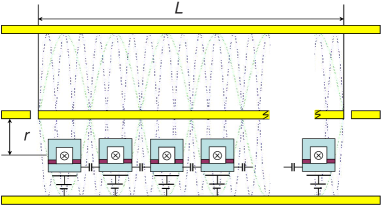
Figure 1: (color online) Schematic diagram of superconducting Ising chain interacting with two largely detuned modes ($\omega_{1}=3\omega_{2}$) individually transmitted in the TLR. Since the CPBs are located at the antinodes of both modes, i.e, $x_{j}=(j-1/2)\pi c/\omega_{2}$, they only interact with the magnetic fields.

In a one dimensional TLR, the electric current and voltage at the position $x$ are given as

$$I(x,t) =\sum_{k}\sqrt{\frac{\hbar\omega_{k}}{Ll}}(a_{k}^{\dagger}+a_{k})\sin(\frac{k\pi x}{L})\text{,}$$ (2)

$$V(x,t) =-i\sum_{k}\sqrt{\frac{\hbar\omega_{k}}{Lc}}(a_{k}^{\dagger}-a_{k})\cos(\frac{k\pi x}{L})\text{,}$$ (3)

where $a_{k}^{\dagger}$ is the creation operator with frequency $\omega_{k}$, $L$ the length of TLR, $l$ and $c$ the induction and capacitance of per unit length of TLR respectively, $k$ positive integer. Therefore, a CPB located at the antinode is only coupled to the magnetic field since the electric field vanishes. According to Ampere’s circuital law, when a dc SQUID loop is placed at a distance $r$ with respect to the center of the TLR, the quantum magnetic flux that threads it is

$$\Phi_{q}(x) =\frac{\mu_{0}IS}{2\pi r}$$

$$=\sum_{k}\frac{\mu_{0}S}{2\pi r}\sqrt{\frac{\hbar\omega_{k}}{Ll}}(a_{k}^{\dagger}+a_{k})\sin(\frac{k\pi x}{L})\text{,}$$ (4)

where $\mu_{0}$ is the vacuum magnetic permeability, $S$ the area of dc SQUID loop.

The interaction between the CPBs and the magnetic field is written as

$$H_{\Phi}=E_{J}\sum_{j}\cos(\frac{\pi\Phi_{q}(x_{j})}{\Phi_{0}})\sigma^{x}_{j}\text{.}$$ (5)

In our consideration, two independent modes with frequencies $\omega_{1}=3\omega_{2}$ are propagating in the TLR. All the CPBs are placed the antinodes of the both modes with the positions

$$x_{j}=\frac{(j-1/2)\pi v}{\omega_{2}}\text{,}$$ (6)

where

$$\omega_{2}=\frac{\pi vL}{M}\text{,}$$ (7)

$j$ and $M$ are positive integers, $v$ the velocity of the light.

Since $\Phi_{q}\ll\Phi_{0}$, under the rotating wave approximation Scully , the interaction Hamiltonian is approximated to the second order,

$$H_{\Phi}=E_{J}[(1-\frac{1}{2}\eta_{1}^{2}-\frac{1}{2}\eta_{2}^{2})-\eta_{1}^{2}a_{1}^{\dagger}a_{1}-\eta_{2}^{2}a_{2}^{\dagger}a_{2}]\sum_{j}\sigma_{j}^{x}\text{,}$$ (8)

where the coupling constants between the two modes and individual spins are

$$\eta_{k}=\frac{\pi\mu_{0}S}{2\pi r\Phi_{0}}\sqrt{\frac{\hbar\omega_{k}}{Ll}}\text{.}$$ (9)

For realistic parameters, $C_{\Sigma}=600$ aF, $C_{m}=30$ aF, $L_{0}=1$ cm, $S_{0}=10\mu m^{2}$, $r=1\mu m$, $N=500$, $E_{J}=13$ GHz, we have $B=1.6$ GHz, $\omega_{2}\approx 120$ GHz, $\eta_{1}=\sqrt{3}\eta_{2}$, and $\eta_{2}\approx 0.1$ Wang07 .

Thus, the total Hamiltonian is written as

$$H= E_{J}[(1-\frac{1}{2}\eta_{1}^{2}-\frac{1}{2}\eta_{2}^{2})-\eta_{1}^{2}a_{1}^{\dagger}a_{1}-\eta_{2}^{2}a_{2}^{\dagger}a_{2}]\sum_{j}\sigma_{j}^{x}$$

$$+\frac{e^{2}C_{m}}{C_{\Sigma}^{2}}\sum_{j}\sigma_{j}^{z}\sigma_{j+1}^{z}+\omega_{1}a_{1}^{\dagger}a_{1}+\omega_{2}a_{2}^{\dagger}a_{2}\text{.}$$ (10)

Furthermore, since there is no energy exchange between the fields and the ICTF, the total Hamiltonian can be decomposed into invariant subspaces with respect to the Fock state of the fields,

$$H=\sum_{m,n}H^{(m,n)}|m\rangle|n\rangle\langle n|\langle m|$$ (11)

where

$$H^{(m,n)}=B\sum\limits_{j=1}^{N}(\lambda_{m,n}\sigma_{j}^{x}+\sigma_{j}^{z}\sigma_{j+1}^{z})$$ (12)

with $B=e^{2}C_{m}/C_{\Sigma}^{2}$ and $\lambda_{m,n}=E_{J}[1-(m+1/2)\eta_{1}^{2}-(n+1/2)\eta_{2}^{2})]/B$.

Generally speaking, the Hamiltonian of ICTF $H_{0}$ is transformed into a quadratic fermion form with Jordan-Wigner transformation Sachdev

$$c_{j}=\exp(\pi i\sum\limits_{k=1}^{j-1}\sigma_{k}^{z})\sigma_{j}^{+}\text{.}$$ (13)

Then, by introducing quasi-particle operator Pfeuty

$$\gamma_{k}=\sum\limits_{j=1}^{N}\frac{e^{-ikj}}{\sqrt{N}}[\cos\frac{\theta_{k}}{2}c_{j}-i\sin\frac{\theta_{k}}{2}c_{j}^{\dagger}]\text{,}$$ (14)

with

$$\theta_{k}(\lambda)=\tan^{-1}\frac{\sin k}{\lambda-\cos k}\text{,}$$ (15)

$H_{0}$ is diagonalized as

$$H_{0}=\sum\limits_{k}\varepsilon_{k}(\gamma_{k}^{\dagger}\gamma_{k}-\frac{1}{2})$$ (16)

with single particle spectrum being

$$\varepsilon_{k}(\lambda)=2B\sqrt{1+\lambda^{2}-2\lambda\cos k}\text{.}$$ (17)

And the ground state $|G\rangle$ corresponds to no quasi-particle excitation at all.

III Photon Bunching Effect

Followed by a series of advances, i.e., resonance fluorescence, the Hanbury-Brown-Twiss experiment Hanbury-Brown reopen philosophical debate about photons Knight and set itself as the milestone in the development of quantum optics. All these experimental phenomena are associated with the correlation functions of the field. Here, we consider it as the method to detect the QPT since the two fields propagating in the TLR interact with the quasi-spins respectively.

First of all, we define an operator

$$A=a_{1}+ia_{2}\text{.}$$ (18)

The first order correlation function is written as $\langle A^{\dagger}(t)A\rangle$. Here, the bracket $\langle\cdots\rangle$ denotes average over the initial state, with the Ising chain in the ground state $|G\rangle$ and the two fields being in arbitrary pure states $\sum_{m}c_{m}|m\rangle$ and $\sum_{n}d_{n}|n\rangle$ respectively. Therefore,

$$\langle A^{\dagger}(t)A\rangle= \sum\limits_{m,n}|c_{m}|^{2}|d_{n}|^{2}(mr^{(m,n)}_{m-1,n}+nr^{(m,n)}_{m,n-1})$$

$$-ic_{m-1}^{*}c_{m}d_{n+1}^{*}d_{n}\sqrt{m(n+1)}r^{(m-1,n+1)}_{m-1,n}$$

$$+ic_{m+1}^{*}c_{m}d_{n-1}^{*}d_{n}\sqrt{(m+1)n}r^{(m+1,n-1)}_{m,n-1}$$ (19)

where

$$r^{(m,n)}_{m^{\prime},n^{\prime}}(t)=\langle G|e^{iH^{(m,n)}t}e^{-iH^{(m^{\prime},n^{\prime})}t}|G\rangle$$ (20)

is the decoherence factor Quan06 which measures the overlap of the ground state evolving under two different Hamiltonians. Details about its calculation is presented in Appendix A. In Ref.Wang07 , it was discovered that for the same amount of environment dissipation the first order correlation function of the single mode decreased more rapidly in the vicinity of the QPT than in the other region.

Moreover, the second order correlation function $\langle A^{\dagger}A^{\dagger}(t)A(t)A\rangle$ is analytically written as

$$\langle A^{\dagger}A^{\dagger}(t)A(t)A\rangle=$$

$$\sum\limits_{m,n} |c_{m}|^{2}|d_{n}|^{2}[(m+n)(m+n-1)+mnr^{(m-1,n)}_{m,n-1}e^{-i(\omega_{1}-\omega_{2})t}+mnr^{(m,n-1)}_{m-1,n}e^{i(\omega_{1}-\omega_{2})t}]$$

$$+ic_{m+1}^{*}c_{m}d_{n-1}^{*}d_{n}\{(m+n-1)\sqrt{(m+1)n}+[m\sqrt{(m+1)n}r^{(m,n-1)}_{m-1,n}+(n-1)\sqrt{(m+1)n}r^{(m+1,n-2)}_{m,n-1}]e^{i(\omega_{1}-\omega_{2})t}\}$$

$$-ic_{m-1}^{*}c_{m}d_{n+1}^{*}d_{n}\{(m+n-1)\sqrt{m(n+1)}+[(m-1)\sqrt{m(n+1)}r^{(m-2,n+1)}_{m-1,n}+n\sqrt{m(n+1)}r^{(m-1,n)}_{m,n-1}]e^{-i(\omega_{1}-\omega_{2})t}\}$$

$$-c_{m+2}^{*}c_{m}d_{n-2}^{*}d_{n}\sqrt{(m+2)(m+1)n(n-1)}r^{(m+1,n-2)}_{m,n-1}e^{i(\omega_{1}-\omega_{2})t}$$

$$-c_{m-2}^{*}c_{m}d_{n+2}^{*}d_{n}\sqrt{(m-1)m(n+1)(n+2)}r^{(m-2,n+1)}_{m-1,n}e^{-i(\omega_{1}-\omega_{2})t}\text{.}$$ (21)

Thus, for the fields initially in the state $(|0\rangle+|1\rangle)/\sqrt{2}$, it is straightforward to obtain

$$\langle A^{\dagger}A^{\dagger}(t)A(t)A\rangle=\frac{1}{2}[1+\text{Re}(r^{(1,0)}_{0,1}e^{i(\omega_{1}-\omega_{2})t)})]\text{,}$$ (22)

where Re$(x)$ means the real part of $x$.

As proven in Appendix A, in the vicinity of the QPT, the square of the norm of $r^{(1,0)}_{0,1}(t)$ decreases more rapidly than exponential, i.e,

$$|r^{(1,0)}_{0,1}(t)|^{2}\leq e^{-\gamma t^{2}}\text{,}$$ (23)

where $\gamma=4B^{2}(\lambda_{1,0}-\lambda_{0,1})^{2}E(k_{c})/(\lambda_{0,1}-1)^{2}$, $E(k_{c})=4\pi^{2}N_{c}(N_{c}+1)(2N_{c}+1)/6N^{2}$ with $N_{c}$ being the nearest integer to $Nk_{c}/2\pi$.

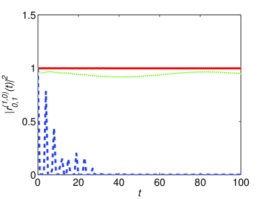
Figure 2: (color online) The decoherence factor $|r^{(1,0)}_{0,1}(t)|^{2}$ for both fields in $(|0\rangle+|1\rangle)/\sqrt{2}$ is plotted with $N=8000$. Blue dashed line for $\lambda=1$, red solid line for $\lambda=0.1$, and green dotted line for $\lambda=2$. In all figures, $t$ is in units of $1/B$.

It can be seen that there is a vanishing numerator $E(k_{c})$ as $N\rightarrow\infty$. It is doubtful that the exponential decay of $|r^{(1,0)}_{0,1}(t)|^{2}$ can truly occur since the QPT takes place in the thermodynamical limit. However, as the size of the ICTF gets larger, we can adjust the parameter $\lambda_{0,1}$ closer to the critical point to make the denominator $(\lambda_{0,1}-1)^{2}$ small enough. In that case, $\gamma$ stays as a constant and the $|r^{(1,0)}_{0,1}(t)|^{2}$ decreases exponentially with time. For a real system, $N$ is finite for the demonstration of the QPT. To test the validity of the above analysis, we resort to numerical simulation. In Fig.2, we plot the evolution of $|r^{(1,0)}_{0,1}(t)|^{2}$ according to Eq.(34). It can be seen that despite some oscillations $|r^{(1,0)}_{0,1}(t)|^{2}$ decays exceptionally at the critical point.

According to Ref.Scully , the photon bunching and anti-bunching effects are associated with the second order degree of coherence

$$g^{(2)}(t)=\frac{\langle A^{\dagger}A^{\dagger}(t)A(t)A\rangle}{\langle A^{\dagger}A\rangle\langle A^{\dagger}(t)A(t)\rangle}\text{,}$$ (24)

which is the normalized second order correlation function of the fields. For the fields both in the state $(|0\rangle+|1\rangle)/\sqrt{2}$, the second order degree of coherence is simplified as

$$g^{(2)}(t)=\frac{1}{2}\frac{1+\text{Re}(r^{(1,0)}_{0,1}e^{i(\omega_{1}-\omega_{2})t})}{1-\text{Im}(r^{(1,0)}_{0,1}e^{i(\omega_{1}-\omega_{2})t})}$$ (25)

with Im$(x)$ being the image part of $x$.

Since the norm of the decoherence factor decreases exponentially at the critical point, it is obvious that both the real and image parts of $r^{(1,0)}_{0,1}e^{i(\omega_{1}-\omega_{2})t}$ will vanish in that limit. As a consequence, we expect the second order degree of coherence to be less than unity in the steady state, i.e., $g^{(2)}(t)=1/2<g^{(2)}(0)=1$. Generally speaking, classical fields such as thermal light and coherent light, prefer to distribute themselves in bunches rather than at random. They exhibit less correlation for time longer than the correlation time. This is so called bunching effect Scully . On the contrary, in certain quantum optical systems, fewer quantum photons are detected close together than further apart. And the photon antibunching observed in fluorescent light from a two-level atom Knight is of such kind. Here, since the two fields involved are two independent modes, we expect photons to be neither bunching nor antibunching, regardless of quantum mechanical fields or classical fields. However, as shown in Fig.3, when the Ising chain is at the critical point, the two independent fields initially in $(|0\rangle+|1\rangle)/\sqrt{2}$ display the photon bunching effect. Further witness is also demonstrated in Fig.4(a-c). It can also be proven that $g^{(2)}(t)<g^{(2)}(0)$ for both fields in the coherent state $|\alpha\rangle$ which is not shown here. In Fig.4(d), we plot the time evolution of the second order of coherence for this case. Here, we remark that the two initially independent quantum fields display the classical effect due to their common interaction with the quantum critical system. As illustrated in Eq.(20), two initially identical states evolve under two slightly different Hamiltonians. Although the difference between these Hamiltonians are tiny, their evolution trajectories are quite distinct in the vicinity of the QPT. Thus, this slight difference leads to the exponential decay of their decoherence factor. It can be understood as a signature of quantum chaos Quan06 .

Furthermore, for the parameters mentioned after Eq.(9) and $N_{c}=N/10$, both the real and imaginary parts of $r^{(1,0)}_{0,1}e^{i(\omega_{1}-\omega_{2})t}$ decay with a rate of the order $\sqrt{\gamma}\simeq 2.5$ GHz. Since the dissipation rate of the first excitation mode is about $6.3$ MHz Wallraff , we can neglect the influence due to the dissipation of TLR.

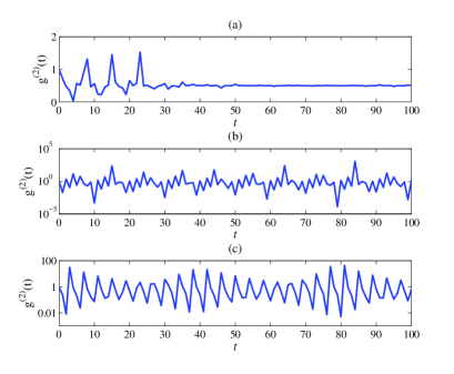
Figure 3: (color online) The second order degree of coherence $g^{(2)}(t)$ for $N=4000$ and $(|0\rangle+|1\rangle)/\sqrt{2}$ is plotted with (a) $\lambda=1$, (b) $\lambda=0.1$, (c) $\lambda=2$.

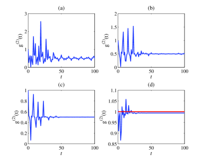
Figure 4: (color online) The second order degree of coherence $g^{(2)}(t)$ is plotted at the critical point for $(|0\rangle+|1\rangle)/\sqrt{2}$ with (a) $N=2000$, (b) $N=4000$, (c) $N=8000$. For (d), both fields are in the coherent states $|\alpha\rangle$ with $\alpha=1$ and $N=8000$. Note that at the steady state $g^{(2)}(t)$ is a little smaller than its original value $1$ as indicated by the red horizontal line.

IV Conclusion and Remark

To conclude, we have explored the possibility to probe quantum criticality in the ICTF by detecting the higher order quantum coherence of the two modes of cavity fields coupled to the spins. We suggest a physical implementation of this theoretical scheme based on a circuit QED system where the capacitively coupled CPBs are coupled to the TLR. Situated at the antinodes of both modes propagating in the TLR, CPBs are only coupled to the magnetic fields. In a heuristic way, we show the decoherence factor decays exponentially with time in the vicinity of the critical point. The second order of coherence is smaller than one at the steady state. Thus, the two initially independent modes demonstrate photon bunching effect. This can serve as a witness of the QPT.

On the other hand, we have not investigated decoherence originated from the dissipation of the CPBs. We notice that in a recent work Hoyos , the QPT in the dissipative random transverse-field Ising chain was investigated. It was discovered that the quantum critical point was ruined by the interplay between quantum fluctuations and Ohmic dissipation. Further exploration may be done when such kind of effect is considered.

Appendix A Decoherence Factor

Following the method introduced in Ref.Wang07 , the decoherence factor $r^{(m,n)}_{m^{\prime},n^{\prime}}$ can be calculated in the following way.

By introducing the spin-1 pseudospin operators Anderson

$$s_{xk} =i(\gamma_{-k}\gamma_{k}+\gamma_{-k}^{\dagger}\gamma_{k}^{\dagger})\text{,}$$

$$s_{yk} =\gamma_{-k}^{\dagger}\gamma_{k}^{\dagger}-\gamma_{-k}\gamma_{k}\text{,}$$

$$s_{zk} =\gamma_{k}^{\dagger}\gamma_{k}+\gamma_{-k}^{\dagger}\gamma_{-k}-1\text{,}$$ (26)

the Hamiltonian $H_{0}$ can also be rewritten as

$$H_{0}=\sum\limits_{k>0}\varepsilon_{k}s_{zk}\text{.}$$ (27)

Because there is no energy exchange between the two modes and the qubit array, the total Hamiltonian can be decomposed into invariant subspaces with respect to the Fock state of the fields, i.e., $H=\sum_{m,n}H^{(m,n)}|m\rangle|n\rangle\langle n|\langle m|$, where

$$H^{(m,n)}=B\sum\limits_{j=1}^{N}(\lambda_{m,n}\sigma_{j}^{x}+\sigma_{j}^{z}\sigma_{j+1}^{z})\text{.}$$ (28)

With the pseudospin operators, we can also diagonalize the Hamiltonian as

$$H^{(m,n)}=\sum\limits_{k>0}\varepsilon_{k}^{(m,n)}s^{(m,n)}_{zk}\text{,}$$ (29)

where $s^{(m,n)}_{zk}=s_{zk}\cos 2\alpha^{(m,n)}_{k}+s_{xk}\sin 2\alpha^{(m,n)}_{k}$ , with $2\alpha^{(m,n)}_{k}=\theta^{(m,n)}_{k}-\theta_{k}$, $\varepsilon^{(m,n)}_{k}=\varepsilon_{k}(\lambda_{m,n})$, $\theta^{(m,n)}_{k}=\theta_{k}(\lambda_{m,n})$.

Therefore, the ground state of $H_{0}$ is the product state of all pseudospins down $|-\rangle_{k}$,

$$|G\rangle =\prod\limits_{k>0}^{\bigotimes}|-\rangle_{k}$$

$$=\prod\limits_{k>0}^{\bigotimes}(\cos\alpha^{(m,n)}_{k}|-\rangle^{(m,n)}_{k}+\sin\alpha^{(m,n)}_{k}|+\rangle^{(m,n)}_{k})$$ (30)

with $|\pm\rangle^{(m,n)}_{k}$ being the eigen states of $s^{(m,n)}_{zk}$.

Since

$${}_{k}^{(m,n)}\langle\pm|\pm\rangle_{k^{\prime}}^{(m^{\prime},n^{\prime})} =\delta_{kk^{\prime}}\cos(\alpha_{k}^{(m,n)}-\alpha_{k}^{(m^{\prime},n^{\prime})})\text{,}$$

$${}_{k}^{(m,n)}\langle+|-\rangle_{k^{\prime}}^{(m^{\prime},n^{\prime})} =\delta_{kk^{\prime}}\sin(\alpha_{k}^{(m,n)}-\alpha_{k}^{(m^{\prime},n^{\prime})})\text{,}$$

$${}_{k}^{(m,n)}\langle-|+\rangle_{k^{\prime}}^{(m^{\prime},n^{\prime})} =\delta_{kk^{\prime}}\sin(\alpha_{k}^{(m^{\prime},n^{\prime})}-\alpha_{k}^{(m,n)})\text{,}$$ (31)

we have

$$r^{(m,n)}_{m^{\prime},n^{\prime}}(t)=\prod\limits_{k>0}\sum\limits_{a_{k},b_{k}=\pm}C_{a_{k},b_{k},k}^{(m,n,m^{\prime},n^{\prime})}e^{i(a_{k}\varepsilon_{k}^{(m,n)}+b_{k}\varepsilon_{k}^{(m^{\prime},n^{\prime})})t}$$ (32)

with

$$C_{+,+,k}^{(m,n,m^{\prime},n^{\prime})} =\sin\alpha_{k}^{(m,n)}\cos\alpha_{k}^{(m^{\prime},n^{\prime})}\sin(\alpha_{k}^{(m,n)}-\alpha_{k}^{(m^{\prime},n^{\prime})})\text{,}$$

$$C_{-,-,k}^{(m,n,m^{\prime},n^{\prime})} =\cos\alpha_{k}^{(m,n)}\sin\alpha_{k}^{(m^{\prime},n^{\prime})}\sin(\alpha_{k}^{(m^{\prime},n^{\prime})}-\alpha_{k}^{(m,n)})\text{,}$$

$$C_{+,-,k}^{(m,n,m^{\prime},n^{\prime})} =\sin\alpha_{k}^{(m,n)}\sin\alpha_{k}^{(m^{\prime},n^{\prime})}\cos(\alpha_{k}^{(m,n)}-\alpha_{k}^{(m^{\prime},n^{\prime})})\text{,}$$

$$C_{-,+,k}^{(m,n,m^{\prime},n^{\prime})} =\cos\alpha_{k}^{(m,n)}\cos\alpha_{k}^{(m^{\prime},n^{\prime})}\cos(\alpha_{k}^{(m,n)}-\alpha_{k}^{(m^{\prime},n^{\prime})})\text{.}$$

For heuristic analysis, we obtain the short time behavior of $|r^{(1,0)}_{0,1}(t)|^{2}$ at the critical point.

$$|r^{(1,0)}_{0,1}(t)|^{2}=\prod\limits_{k>0} F_{k}$$

$$=\prod\limits_{k>0} [\sin^{2}(\alpha_{k}^{(1,0)}-\alpha_{k}^{(0,1)})\cos(\varepsilon_{k}^{(1,0)}+\varepsilon_{k}^{(0,1)})t+\cos^{2}(\alpha_{k}^{(1,0)}-\alpha_{k}^{(0,1)})\cos(\varepsilon_{k}^{(1,0)}-\varepsilon_{k}^{(0,1)})t]^{2}$$

$$+[\sin(\alpha_{k}^{(1,0)}+\alpha_{k}^{(0,1)})\sin(\alpha_{k}^{(1,0)}-\alpha_{k}^{(0,1)})\cos(\varepsilon_{k}^{(1,0)}+\varepsilon_{k}^{(0,1)})t$$

$$-\cos(\alpha_{k}^{(1,0)}+\alpha_{k}^{(0,1)})\cos(\alpha_{k}^{(1,0)}-\alpha_{k}^{(0,1)})\sin(\varepsilon_{k}^{(1,0)}+\varepsilon_{k}^{(0,1)})t]^{2}$$ (34)

Since all factors $F_{k}$ of $|r^{(1,0)}_{0,1}(t)|^{2}$ have a norm less than unity, we may expect the $|r^{(1,0)}_{0,1}(t)|^{2}$ to vanish under certain conditions. Here, we set a cutoff frequency $k_{c}$ and hence we have $|r^{(1,0)}_{0,1}(t)|^{2}\leq\prod\limits_{k>0}^{k_{c}}F_{k}$. For small $k$, we have

$$\varepsilon_{k}^{(1,0)} \approx 2B|1-\lambda_{1,0}|\text{,}$$

$$\varepsilon_{k}^{(0,1)} \approx 2B|1-\lambda_{0,1}|\text{,}$$

$$\theta_{k}(\lambda) \approx\frac{k}{\lambda-1}\text{,}$$

$$\alpha_{k}^{(1,0)} \approx\frac{1}{2}(\frac{k}{\lambda_{1,0}-1}-\frac{k}{\lambda_{0,0}-1})\text{,}$$

$$\alpha_{k}^{(0,1)} \approx\frac{1}{2}(\frac{k}{\lambda_{0,1}-1}-\frac{k}{\lambda_{0,0}-1})\text{.}$$

To the second order of $\alpha_{k}^{(1,0)}\pm\alpha_{k}^{(0,1)}$, we obtain

$$|r^{(1,0)}_{0,1}(t)|^{2}$$

$$\leq\prod\limits_{k>0}^{k_{c}}[1-2(\alpha_{k}^{(1,0)}-\alpha_{k}^{(0,1)})^{2}]\cos^{2}(\varepsilon_{k}^{(1,0)}-\varepsilon_{k}^{(0,1)})t$$

$$+2(\alpha_{k}^{(1,0)}-\alpha_{k}^{(0,1)})^{2}\cos(\varepsilon_{k}^{(1,0)}+\varepsilon_{k}^{(0,1)})t\cos(\varepsilon_{k}^{(1,0)}-\varepsilon_{k}^{(0,1)})t$$

$$+[1-(\alpha_{k}^{(1,0)})^{2}-(\alpha_{k}^{(0,1)})^{2}]\sin^{2}(\varepsilon_{k}^{(1,0)}-\varepsilon_{k}^{(0,1)})t$$

$$-2[(\alpha_{k}^{(1,0)})^{2}-(\alpha_{k}^{(0,1)})^{2}]\sin(\varepsilon_{k}^{(1,0)}-\varepsilon_{k}^{(0,1)})t$$

$$\times\sin(\varepsilon_{k}^{(1,0)}+\varepsilon_{k}^{(0,1)})t\text{.}$$

Since

$$0\approx\varepsilon_{k}^{(1,0)}-\varepsilon_{k}^{(0,1)}\ll\varepsilon_{k}^{(1,0)}+\varepsilon_{k}^{(0,1)}\approx 2\varepsilon_{k}^{(1,0)}\text{,}$$

we focus on the short time behavior and therefore

$$|r^{(1,0)}_{0,1}(t)|^{2}$$

$$\leq\prod\limits_{k>0}^{k_{c}}[1-2(\alpha_{k}^{(1,0)}-\alpha_{k}^{(0,1)})^{2}]+2(\alpha_{k}^{(1,0)}-\alpha_{k}^{(0,1)})^{2}\cos(2\varepsilon_{k}^{(1,0)}t)$$

$$=\prod\limits_{k>0}^{k_{c}}1-2(\alpha_{k}^{(1,0)}-\alpha_{k}^{(0,1)})^{2}\sin^{2}(\varepsilon_{k}^{(1,0)}t)$$

$$=\prod\limits_{k>0}^{k_{c}}1-2\frac{k^{2}(\lambda_{1,0}-\lambda_{0,1})^{2}}{(\lambda_{1,0}-1)^{2}(\lambda_{0,1}-1)^{2}}\sin^{2}(2Bt|\lambda_{1,0}-1|)\text{.}$$

As $\lambda_{1,0}\rightarrow 1$, we have

$$|r^{(1,0)}_{0,1}(t)|^{2}\leq e^{-\gamma t^{2}}\text{,}$$ (35)

where $\gamma=4B^{2}(\lambda_{1,0}-\lambda_{0,1})^{2}E(k_{c})/(\lambda_{0,1}-1)^{2}$, $E(k_{c})=4\pi^{2}N_{c}(N_{c}+1)(2N_{c}+1)/6N^{2}$ with $N_{c}$ being the nearest integer to $Nk_{c}/2\pi$.

References

• (1) A. Osterloh, L. Amico, G. Falci, and R. Fazio, Nature (London) 416, 608 (2002).
• (2) Shi-Jian Gu, Shu-Sa Deng, You-Quan Li, and Hai-Qing Lin,Phys. Rev. Lett. 93, 086402 (2004).
• (3) S. Sachdev, Quantum Phase Transition, (Cambridge University Press, Cambridge, England, 1999).
• (4) C. Emary and T. Brandes, Phys. Rev. Lett. 90, 044101 (2003)
• (5) Yong Li, Z. D. Wang, and C. P. Sun,Phys. Rev. A 74, 023815 (2006).
• (6) H. T. Quan, Z. Song, X. F. Liu, P. Zanardi, and C. P. Sun, Phys. Rev. Lett. 96, 140604 (2006).
• (7) A. Peres, Quantum Theory: Concepts and Methods, (Kluwer Academic Publishers, New York, 2002).
• (8) A. Wallraff, D. I. Schuster, A. Blais, L. Frunzio, R. S. Huang, J. Majer, S. Kumar, S. M. Girvin, and R. J. Schoelkopf, Nature (London) 431, 162 (2004).
• (9) I. Chiorescu, P. Bertet, K. Semba, Y. Nakamura, C. J. P. M. Harmans, J. E. Mooij, Nature (London) 431, 159 (2004).
• (10) J. Q. You, F. Nori, Physics Today 58, 42 (2005).
• (11) K. Moon and S. M. Girvin, Phys. Rev. Lett. 95, 140504 (2005).
• (12) Y.D. Wang, F. Xue, Z. Song, and C. P. Sun, Phys. Rev. B 76, 174519 (2007).
• (13) J. F. Zhang, X. H. Peng, N. Rajendran, and D. Suter, Phys. Rev. Lett. 100, 100501 (2008).
• (14) M. O. Scully, M. S. Zubairy, Quantum Optics, (Cambridge University Press, Cambridge, England, 1997).
• (15) P. Pfeuty, Ann. Phys. (N.Y.) 57, 79 (1970).
• (16) H. Hanbury-Brown and R. Q. Twiss, Phil. Mag. 45, 663 (1954); Nature 178, 1046 (1956); Proc. Roy. Soc. A242, 300 (1957).
• (17) P. L. Knight and L. Allen, Concepts of Quantum Optics, (Pergamon Press, Oxford, 1983).
• (18) J. A. Hoyos and T. Vojta, Phys. Rev. Lett. 100, 240601 (2008).
• (19) P. W. Anderson, Phys. Rev. 112, 1900 (1958).