Scattering polarization due to light source anisotropy

Abstract

Aims. We consider the polarization arising from scattering in an envelope illuminated by a central anisotropic source. This work extends the theory introduced in a previous paper (Al-Malki et al. 1999) in which scattering polarization from a spherically symmetric envelope illuminated by an anisotropic point source was considered. Here we generalize to account for the more realistic expectation of a non-spherical envelope shape.

Methods. Spherical harmonics are used to describe both the light source anisotropy and the envelope density distribution functions of the scattering particles. This framework demonstrates how the net resultant polarization arises from a superposition of three basic “shape” functions: the distribution of source illumination, the distribution of envelope scatterers, and the phase function for dipole scattering.

Results. Specific expressions for the Stokes parameters and scattered flux are derived for the case of an ellipsoidal light source inside an ellipsoidal envelope, with principal axes that are generally not aligned. Two illustrative examples are considered: (a) axisymmetric mass loss from a rapidly rotating star, such as may apply to some Luminous Blue Variables, and (b) a Roche-lobe filling star in a binary system with a circumstellar envelope.

Conclusions. As a general conclusion, the combination of source anisotropy with distorted scattering envelopes leads to more complex polarimetric behavior such that the source characteristics should be carefully considered when interpreting polarimetric data.

1 Introduction

For many stars linear polarization is produced mainly from scattering of starlight by circumstellar matter (Kruszewski et al. 1968; Serkowski 1970; Dyck et al. 1971; Shawl 1975). This polarization can be used as a diagnostic of the geometry of the circumstellar envelope and of the light source(s) (e.g., Shakhovskoi 1965; Serkowski 1970; Brown & McLean 1977; Brown et al. 1978; Rudy & Kemp 1978; Simmons 1982, 1983; Friend & Cassinelli 1986; Clarke & McGale 1986, 1987). In many models for circumstellar scattering polarization, the illuminating sources are treated as isotropic point sources (e.g., Brown & McLean 1977; Brown et al. 1978; Rudy & Kemp 1978; Shawl 1975; Simmons 1982). The effect of the finite size of the star as a light source has been studied (Cassinelli, Nordsieck, & Murison 1987), including the effects of limb darkening (Brown et al. 1989) and stellar occultation (Brown & Fox 1989; Fox & Brown 1991; Fox 1991). Variable polarization is also revealing about a system, as evidenced in a recent study by Elias, Koch, & Pfeiffer (2008). With recent emphasis on clumped wind flows of hot stars (e.g., Hamann, Feldmeier, & Oskinova 2008), models have been developed to interpret variable polarization from hot star winds (Richardson, Brown, & Simmons 1996; Brown, Ignace, & Cassinelli 2000; Li et al. 2000; Davies et al. 2007).

Relatively little has been done to explore the anisotropy of the source illumination and its consequences for interpreting polarimetric observations. There are some exceptions, such as a study of gravity-darkening effects for the polarization from Be stars by Bjorkman & Bjorkman (1994), the influence of star spots for polarizations from pre-main sequence stars by Vink et al. (2005), and more recently calculations of source anisotropy for interpreting polarimetric behavior observed in the post-red supergiant star HD 179821 by Patel et al. (2008). In a previous paper (Al-Malki et al. 1999; hereafter Paper I), we modeled the polarization arising from Thomson and Rayleigh scattering explicitly for an arbitrary anisotropic (point) light source. As a proof of concept, the circumstellar envelope was taken as spherically symmetric to explore the polarization signals that arise solely from the properties of the source. An upper limit to the polarization of about 20% was derived in the limiting case of a disk-like star when viewed edge-on.

This paper generalizes the results of Paper I by allowing both the point light source and the particle density distribution to be functions of arbitrary angular form. As in Paper I, we restrict ourselves to optically thin envelopes and single Thomson or Rayleigh scattering mechanisms. Although the effects of a finite-sized illuminator will be important for obtaining quantitatively a more accurate polarization amplitude (e.g., Ignace, Henson, & Carson 2008), the point source approximation is certainly adequate for exploring polarization trends of generalized source and envelope geometries. In Sect. 2, we develop the theory required to evaluate the polarization, based on Paper I and the discussion of Simmons (1982). Applications to specific cases of astrophysical interest are explored in Sect. 3, with emphasis given to a treatment of the star and the circumstellar envelope as ellipsoidal. A discussion of these results and the need for ongoing modeling is given in Sect. 4.

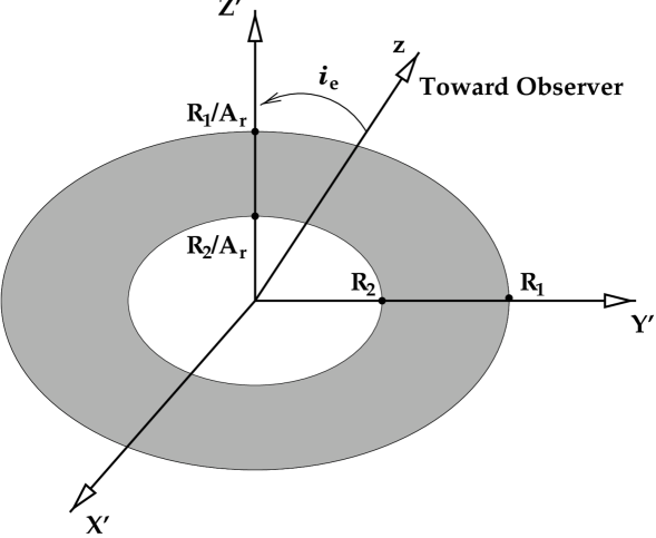
Figure 1: Illustration of the ellipsoidal envelope used in our models. The scattering envelope is shown in cross-section as shaded, with an equatorial width ranging from an inner radius of $R_{2}$ to an outer one of $R_{1}$. Along the pole, the inner and outer boundaries are scaled by the factor $A_{\rm r}$. Although the theory allows for fully triaxial ellipsoids, our specific applications are for axisymmetric ellipsoids (ranging from oblate to prolate).

2 General expression for scattered flux and polarization

As in Paper I, we neglect the effects of finite star depolarization and stellar occultation. Consequently scattering particles in the circumstellar envelope “see” a point star. However, we model the anisotropy of the illumination with a “shape” function to represent directional flux.

Under these approximations, our goal is to derive the net polarization from dipole scattering for an unresolved system that allows for an arbitrary circumstellar envelope geometry and source geometry. Our approach is to represent the different geometrical factors in terms of expansions in spherical harmonics. As a result, it is important to be clear about the different coordinate systems being employed.

Following the notation of Paper I, a description of the problem requires three coordinate systems, each centered on the star: one for the observer, one for the envelope, and one for the illumination pattern of the star itself. In general, none of these systems are collinear. The systems are defined as follows:

• For the observer reference frame we define Cartesian coordinates $(x,y,z)$ centered at the star, with spherical coordinates $(r,\theta,\phi)$, the line-of-sight being the $Oz-$axis. Thus $\hat{z}$ is a unit vector in the direction of the observer from the star and $x,y$ are observer coordinates in the plane of the sky. For a scattering point in direction $\hat{r}$, the scattering angle is given by $\cos\theta=\hat{z}\cdot\hat{r}$, as in Paper I. The angle $\phi=\tan^{-1}y/x$ is the observer’s polarization angle (orientation) for any scattering point.

• The star’s frame is $(X,Y,Z)$ with spherical coordinates $(r,\vartheta,\varphi)$, where $OZ$ is a convenient stellar axis (such as a rotation axis) that lies in the $x-z$ plane of the observer’s frame. The star system is rotated relative to the observer coordinates $(x,y,z)$ through standard Euler angles $(\alpha,\beta,\gamma)$.

• The envelope frame $(X^{\prime},Y^{\prime},Z^{\prime})$ with spherical coordinates $(r,\vartheta^{\prime},\varphi^{\prime})$, centered on the star, where $OZ^{\prime}$ is a convenient axis for the envelope.

In general the scatterer density is $n(r,\vartheta^{\prime},\varphi^{\prime})$, and the flux of radiation from the star is $F(r,\vartheta,\varphi)$. The stellar illumination is taken to be unpolarized. In fact, stellar atmospheres may show some low level of intrinsic polarization (Collins 1970); however, the polarization from the circumstellar scattering will be dominated by the Stokes-I component from the source. Following Eq. (1) from Paper I (see also Simmons 1982), the scattered flux and Stokes parameters $(F_{\rm sc},Q,U)$ of the scattered radiation at the Earth (distance $D$) are given in the form:

$$\left.\begin{array}[]{c}F_{\rm sc}\\ Z^{*}\end{array}\right\} = \frac{1}{2k^{2}\,D^{2}}\,\int\int\int\,n(r,\theta^{\prime},\phi^{\prime})\,F(r,\vartheta,\varphi)\,r^{2}\times$$ (6)

$$\left\{\begin{array}[]{l}(i_{1}+i_{2})\\ (i_{1}-i_{2})\,\exp(-2i\phi)\end{array}\right.\,dr\,\sin\theta\,d\theta\,d\phi,$$

with the same definitions as in Paper I, with $Z^{*}=Q-iU$, for $i=\sqrt{-1}$, $k=2\pi/\lambda$ the wave number, and $i_{1}$ and $i_{2}$ the scattering functions as defined by van de Hulst (1957). The circular polarization $V$ is assumed zero. For Thomson (free electrons) or Rayleigh scattering, we have

$$i_{1}\pm i_{2}=\frac{3k^{2}}{8\pi}\,\sigma\,(1\pm\cos^{2}\theta),$$ (7)

where the value of the cross section factor $\sigma$ is chosen according to whether Thomson scattering ($\sigma$ independent of $k$) or Rayleigh scattering ($\sigma\propto k^{4}$) is considered.

Provided that $F$ varies smoothly, it may be expressed in terms of spherical harmonics in the observer frame (see Paper I):

$$F(r,\theta,\phi)=\sum_{l=0}^{\infty}\,\sum_{{\rm m}=-l}^{{\rm m}=l}\,F_{l{\rm m}}(r)\,\sum_{{\rm n}=-l}^{{\rm n}=l}\,R^{l}_{\rm nm}(\alpha,\beta,\gamma)\,Y_{l{\rm n}}(\theta,\phi),$$ (8)

where

$$F_{l{\rm m}}(r)=\int^{1}_{-1}\,\int_{0}^{2\pi}\,F(r,\theta,\phi)\,Y^{*}_{l{\rm m}}(\theta,\phi)\,d(\cos\theta)\,d\phi,$$ (9)

and $R^{l}_{nm}$ represents elements of a rotational matrix (see Paper I).

Similarly, the density distribution of scatterers can also be expanded in terms of spherical harmonics, which becomes

$$n(r,\theta,\phi)=\sum_{l^{\prime}=0}^{\infty}\,\sum_{{\rm m^{\prime}}=-l^{\prime}}^{{\rm m^{\prime}}=l^{\prime}}\,n_{l^{\prime}{\rm m^{\prime}}}(r)\,Y_{l^{\prime}{\rm m^{\prime}}}(\theta,\phi),$$ (10)

where

$$n_{l^{\prime}{\rm m^{\prime}}}(r)=\int^{1}_{-1}\,\int_{0}^{2\pi}\,n(r,\theta^{\prime},\phi^{\prime})\,Y^{*}_{l^{\prime}{\rm m^{\prime}}}(\theta^{\prime},\phi^{\prime})\,d(\cos\theta^{\prime})\,d\phi^{\prime}.$$ (11)

The $Y_{l{\rm n}}(\theta,\phi)$ factors in Eqs. (8) and (10) are as defined in Paper I (c.f., Jackson 1975). For the product of two spherical harmonics, we can express the multipoles of $n(r,\theta,\phi)$ and $F(r,\theta,\phi)$ as:

$$n(r,\theta,\phi)\,F(r,\theta,\phi) = \sum_{ll^{\prime}\,{\rm mm^{\prime}}}\,n_{l^{\prime}{\rm m^{\prime}}}(r)\,F_{l{\rm m}}(r)\,\times$$ (12)

$$Y_{l^{\prime}{\rm m^{\prime}}}(\theta,\phi)\,Y_{l{\rm m}}(\theta,\phi),$$

or as

$$n(r,\theta,\phi)\,F(r,\theta,\phi)=\sum_{l{\rm m}n}\,R^{l}_{\rm nm}\,\sum_{l^{\prime}{\rm m^{\prime}}}\,C^{\rm LM}_{ll^{\prime}\,{\rm nm^{\prime}}}\,Y_{\rm LM}(\theta,\phi).$$ (13)

In this latter expression, the set of $C^{\rm LM}_{ll^{\prime}\,{\rm nm^{\prime}}}$ values are Clebsh-Gordon coefficients, arising from the products of two spherical harmonics. Only terms satisfying the following two conditions contribute to the sum in Eq. (13):

$${\rm n}+{\rm m^{\prime}}=M,$$ (14)

and,

$$|l-l^{\prime}|\leq l\leq l+l^{\prime}.$$ (15)

The coefficients are given by the relation,

$$C^{\rm LM}_{ll^{\prime}\,{\rm nm^{\prime}}} = (-1)^{\rm M}\,\sqrt{\frac{(2l+1)(2l^{\prime}+1)(2L+1)}{4\pi}}\times$$ (20)

$$\,\left(\begin{array}[]{ccc}l&l^{\prime}&L\\ 0&0&0\end{array}\right)\,\left(\begin{array}[]{ccc}l&l^{\prime}&L\\ n&m^{\prime}&M\end{array}\right)$$

(c.f., Messiah 1962 and the Appendix).

As in Paper I, the scattering factors can be expressed as

$$1+\cos^{2}\theta=\frac{4}{3}\,\left[\sqrt{4\pi}\,Y_{00}+\sqrt{\frac{\pi}{5}}\,Y_{20}(\theta)\right],$$ (21)

and

$$\sin^{2}\theta\,\exp(-2i\phi)=4\,\sqrt{\frac{2\pi}{15}}\,Y_{22}^{*}(\theta,\phi),$$ (22)

so that, upon substitution in the integrals contained in Eq. (6), together with the other expressions above, and using the properties of spherical harmonics, $F_{\rm sc}$ and $Z^{*}$ can be rewritten as:

$$F_{\rm sc} = \frac{\sigma}{4\pi\,D^{2}}\,\sum_{l{\rm mn}}\,R^{l}_{\rm nm}(\alpha,\beta,\gamma)\times$$ (23)

$$\left[\sqrt{4\pi}\,C_{ll^{\prime}nm^{\prime}}^{00}+\sqrt{\frac{\pi}{5}}\,C_{ll^{\prime}nm^{\prime}}^{20}\right]\,S_{ll^{\prime}mm^{\prime}},$$

and

$$Z^{*}=\frac{3\sigma}{4\pi\,D^{2}}\,\sqrt{\frac{2\pi}{15}}\sum_{l{\rm mn}}\,R^{l}_{\rm nm}(\alpha,\beta,\gamma)\,\sum_{l^{\prime}{\rm m^{\prime}}}C_{ll^{\prime}nm^{\prime}}^{22}\,S_{ll^{\prime}mm^{\prime}},$$ (24)

where

$$S_{ll^{\prime}mm^{\prime}}=\int^{\infty}_{0}\,F_{l{\rm m}}(r)\,n_{l^{\prime}{\rm m^{\prime}}}(r)\,r^{2}\,dr.$$ (25)

Thus, the scattered flux and the Stokes parameters can be expressed as sums of increasing order of multipole contribution. This helps to separate the effects of anisotropy in the flux $F$ and in the density distribution $n$, and to study how they can lead to the production of polarization.

If the functions are smooth, the summations will converge rapidly, so the first few terms ($l$ and $l^{\prime}\leq 2$) should provide reasonable approximations for the behavior of the polarization. Due to the conditions of Eqs. (14) and (15), the summation over $l,l^{\prime}$, m, and m’ in Eqs. (23) and (24) will be limited. For example, if the stellar flux and the circumstellar density distribution of scattering particles is symmetric about stellar and envelope polar axes respectively , the values of $S_{ll^{\prime}{\rm mm^{\prime}}}$ will be zero for odd values of $l$ and $l^{\prime}$.

For a spherical envelope with $n(r,\theta,\phi)=n(r)$ and an anisotropic light source, Eqs. (23) and (24) reduce to the forms discussed in Paper I. On the other hand, for an isotropic light source within an envelope of arbitrary shape, the expressions of Brown & McLean (1977) and Simmons (1982) are recovered.

Figure 2: Plots of $f_{l0}$ for the source flux plotted against the parameter $c$ for the anisotropy of the source. Low $c$ implies greater flux along the stellar poles, whereas large $c$ is the opposite case. The left panel shows curves for $l=0$ and $l=2$ as solid, $l=4$ as dashed, and higher $l$ values as dotted (unlabeled) against $\log c$. The right panel shows a blow up around the region of $c=1$ and explicitly labels the higher order curves. Certainly for $c<1$, $l=0$ and 2 are most important.

3 Ellipsoidal light source and ellipsoidal circumstellar envelope

As an illustration of the preceding general formulation, we will take the case of a star of uniform surface brightness, as discussed in Paper I, but now embedded within an ellipsoidally shaped circumstellar envelope. For an isotropic surface intensity $I_{*}$, the flux $F(r,\vartheta,\varphi)$ can be expressed (as seen from a distant point) in terms of the projected area $A_{\rm p}(\vartheta,\varphi)$ of the star as seen from direction $(\vartheta,\varphi)$. In other words we treat the star as an arbitrarily small unpolarized illuminator but describe its anisotropy in terms of a distorted finite shape.

Under this approximation, the flux is given by

$$F(r,\vartheta,\varphi)\approx I_{*}\,\Delta\Omega=I_{*}\,\frac{A_{\rm p}(\vartheta,\varphi)}{r^{2}},$$ (26)

where $I_{*}$ is the isotropic intensity of the stellar surface and $\Delta\Omega$ is the solid angle subtended by the scattering element located a distance $r$ from the star. As a concrete example, we follow Paper I (see their Fig. 2) by introducing star axes $(a,b,c)$ to be along $(X,Y,Z)$. From Paper I, the areal function is

$$A_{\rm p}=\pi\left|\sqrt{(bc\lambda)^{2}+(ac\mu)^{2}+(ab\nu)^{2}}\right|,$$ (27)

where $(\lambda,\mu,\nu)=(\cos\varphi\,\sin\vartheta,\sin\varphi\,\sin\vartheta,\cos\vartheta)$ are the $(X,Y,Z)$ direction cosines for the direction $(\vartheta,\varphi)$. So we obtain

$$F_{l{\rm m}}(r)=\frac{I_{*}}{r^{2}}\,\int_{0}^{\pi}\,\int_{0}^{2\pi}\,A_{\rm p}(\vartheta,\varphi)\,Y^{*}_{l{\rm m}}(\vartheta,\varphi)\,\sin\vartheta\,d\vartheta\,d\varphi.$$ (28)

For the purpose of illustrative calculations, we now adopt simplifications for the description of the illumination pattern and envelope density profile. Following Simmons (1982), we model the envelope as an axisymmetric ellipsoidal shell (oblate or prolate) of arbitrary thickness and constant density. The shell axis of rotational symmetry $OZ^{\prime}$ has inclination angle $i_{\rm e}$ with the line of sight (see Fig 1). An azimuthal angle $\phi_{\rm env}$ describes the orientation of the projected $OZ^{\prime}$ axis in the $x-y$ plane, which is the plane of the sky for the observer. The density prescription for the envelope becomes

$$n_{l^{\prime}{\rm m^{\prime}}}(r)=2\pi\,(R_{1}-R_{2})\,n_{0}\,K_{l^{\prime}}\,Y_{l^{\prime}{\rm m^{\prime}}}(i_{\rm e},\phi_{\rm e}),$$ (29)

where

$$n(r,\vartheta^{\prime},\varphi^{\prime})=\left\{\begin{array}[]{cl}n_{0}&\hskip 12.91663pt\mbox{\rm when}\;r_{2}(\mu)\leq r\leq r_{1}(\mu),\\ 0&\hskip 12.91663pt\mbox{\rm otherwise.}\end{array}\right.$$ (30)

Here $n_{0}$ is the uniform number density of particles within the column bounded by $r_{1}$ and $r_{2}$, where

$$r_{1,2}(\mu)=\frac{R_{1,2}}{\sqrt{1+(A_{\rm r}^{2}-1)\mu^{2}}},$$ (31)

and

$$\mu=\cos{\zeta}.$$ (32)

The lengths $R_{1}$ and $R_{2}$ are the outer and inner equatorial axis lengths, and $A_{\rm r}$ is the ratio of the length of the equatorial width to the polar width (see Fig. 1). The angle $\zeta$ is the angle between the radius vector and the axis of symmetry, which is related to our frames by the addition theorem of spherical harmonics. This explains the appearance of $Y_{l^{\prime}{\rm m^{\prime}}}(i_{\rm e},\phi_{\rm e})$ in Eq. (29) – see Simmons (1982) and Jackson (1975). Finally, $K_{l^{\prime}}$ is given by

$$K_{l^{\prime}}=\int_{-1}^{1}\,\frac{P_{l^{\prime}}(\mu)}{\sqrt{1+(A_{\rm r}^{2}-1)\mu^{2}}}\,d\mu,$$ (33)

where $P_{l^{\prime}}(x)$ are Legendre polynomials.

Inserting Eqs. (28)–(33) into Eq. (25), we obtain

$$S_{ll^{\prime}{\rm mm^{\prime}}}=I_{*}\,N\,f_{l{\rm m}}\,K_{l^{\prime}}\,Y_{ll^{\prime}{\rm m^{\prime}}}(i_{\rm e},\phi_{\rm e}),$$ (34)

where a convenient column density $N$ is introduced as

$$N=2\pi\,(R_{1}-R_{2})\,n_{0},$$ (35)

and

$$f_{l{\rm m}}=\int_{0}^{\pi}\,\int_{0}^{2\pi}\,A_{\rm p}(\vartheta,\varphi)\,Y^{*}_{l{\rm m}}(\vartheta,\varphi)\,\sin\vartheta\,d\vartheta\,d\varphi.$$ (36)

Note that the multipoles of the flux $f_{l{\rm m}}$ are now functions of the star’s effective shape. The multipole coefficients of the envelope $K_{l^{\prime}}$ are functions of the envelope’s shape and size. Conceptually, the product of $K_{l^{\prime}}$ and $f_{l{\rm m}}$ leads to an overall net amplitude “pattern” of scattered light as determined by whether the two functions enhance or offset one another. This pattern sets the contribution level to the polarization and scattered flux as a function of direction about the source. The scattering phase function (in our case dipole scattering) along with appropriate rotations operates as a weighted filter function that acts on the amplitude pattern, converting it to a net observed Stokes vector signal from the source and envelope system.

Describing the orientation of the star relative to the observer frame in terms of the Euler angles, we can choose $\alpha$ as zero, $\beta$ as the viewing inclination ($i_{s}$) of the $OZ-$axis (i.e., the nominal rotation axis of the star) to the line of sight $Oz$, and $\gamma$ as the azimuth of the $OZ-$axis from the $Ox-$axis as measured about the $Oz-$axis, which we denote as $\phi_{\rm s}$. Thus $\phi_{\rm s}$ measures the rotational phase of the star relative to the observer (the same conventions as adopted in Paper I; see their Fig. 1).

In the observational context, it is the normalized scattered flux and Stokes parameters that are usually used. These are given by $(f_{\rm sc},q,u)=(F_{\rm sc},Q,U)/F_{\rm tot}$, where the total flux received $F_{\rm tot}$ comprises the combination of the scattered flux $F_{\rm sc}$ plus direct flux from the star $F_{\ast}$. This contribution by direct stellar light we denote as $F_{\ast}=I_{*}\,A_{\rm p}(i_{\rm s},\phi_{\rm s})/D^{2}$. So the total observed flux becomes

$$F_{\rm tot}=\frac{I_{\ast}}{D^{2}}\,\left[A_{\rm p}(i_{\rm s},\phi_{\rm s})+(D^{2}/I_{\ast})\,F_{\rm sc}\right].$$ (37)

The general expressions for the normalized scattered flux and stokes parameters become

$$f_{\rm sc} = \frac{\tau}{4\pi\,D^{2}\,F_{\rm tot}}\,\sum_{l{\rm mn}}\,R^{l}_{\rm nm}(0,i_{\rm s},\phi_{\rm s})\,f_{l{\rm m}}\times$$ (38)

$$\left[\sqrt{4\pi}C_{ll^{\prime}{\rm nm^{\prime}}}^{00}+\sqrt{\frac{\pi}{5}}C_{ll^{\prime}{\rm nm^{\prime}}}^{20}\right]$$

and

$$z^{*} = \frac{3\tau}{4\pi\,D^{2}\,F_{\rm tot}}\,\sqrt{\frac{2\pi}{15}}\sum_{l{\rm mn}}\,R^{l}_{\rm nm}(0,i_{\rm s},\phi_{\rm s})\,f_{l{\rm m}}$$ (39)

$$\sum_{l^{\prime}{\rm m^{\prime}}}K_{l^{\prime}}\,Y_{l^{\prime}{\rm m}}(i_{\rm e},\phi_{\rm e})\,C_{ll^{\prime}nm^{\prime}}^{22}\,S_{ll^{\prime}mm^{\prime}},$$

where $\tau=\sigma(R_{1}-R_{2})n_{0}$ is the equatorial optical depth. The degree of polarization is given by $p=|z^{*}|=|z|$, and the polarization position angle is given by $\psi=\frac{1}{2}arg\,z$.

From Eqs. (38) and (39), we can calculate the polarization and the scattered flux, using the properties of the two factors $K_{l^{\prime}}$ and $f_{l{\rm m}}$ that describe the envelope geometry and source anisotropy. Due to the symmetry of the functions chosen to describe the stellar flux and the scatterer density distribution, $K_{l^{\prime}}$ and $f_{l{\rm m}}$ are non-zero only for even $l^{\prime}$ and $l$, respectively.

4 Applications

As mentioned above, the multipoles of the flux $f_{l{\rm m}}$ are non-zero only for even $l$, and the spherical harmonics for $l\geq 4$ are important mainly for fairly large angular distortions of the star from sphericity. As an example, Figures 2a and b show the variation of $f_{l0}$ for an oblate/prolate star distorted only along its $c-$axis.

For $l=l^{\prime}=2$, the scattered flux is a sum of terms given by

$$F_{\rm sc} = \frac{\sigma}{4\pi\,D^{2}}\,\left\{\sqrt{4\pi}\,\left[\sum_{\rm m=-2}^{\rm m=2}\,S_{\rm m}^{22\,2-2}\,C^{00}_{22\,2-2}\right.\right.$$ (40)

$$+\sum_{\rm m=-2}^{\rm m=2}\,S_{\rm m}^{22\,1-1}\,C^{00}_{22\,1-1}\sum_{\rm m=-2}^{\rm m=2}\,S_{\rm m}^{22\,00}\,C^{00}_{22\,00}$$

$$+\sum_{\rm m=-2}^{\rm m=2}\,S_{\rm m}^{22\,-11}\,C^{00}_{22\,-11}\sum_{\rm m=-2}^{\rm m=2}\,S_{\rm m}^{22\,-22}\,C^{00}_{22\,-22}$$

$$+S_{\rm m}^{00\,00}\,C^{00}_{00\,00}\left]+\sqrt{\frac{\pi}{5}}\,\right[S_{0}^{02\,00}\,C^{20}_{02\,00}$$

$$+\sum_{\rm m=-2}^{\rm m=2}\,S_{\rm m}^{22\,2-2}\,C^{20}_{22\,2-2}\sum_{\rm m=-2}^{\rm m=2}\,S_{\rm m}^{22\,1-1}\,C^{20}_{22\,1-1}$$

$$+\sum_{\rm m=-2}^{\rm m=2}\,S_{\rm m}^{22\,00}\,C^{20}_{22\,00}\sum_{\rm m=-2}^{\rm m=2}\,S_{\rm m}^{22\,-11}\,C^{20}_{22\,-11}$$

$$\left.\left.+\sum_{\rm m=-2}^{\rm m=2}\,S_{\rm m}^{22\,-22}\,C^{20}_{22\,-22}\sum_{\rm m=-2}^{\rm m=2}\,S_{\rm m}^{20\,00}\,C^{20}_{20\,00}\right]\right\},$$

and the Stokes parameters as

$$Z^{*} = \frac{3\sigma}{4\pi\,D^{2}}\,\sqrt{\frac{2\pi}{15}}\,\left\{S_{0}^{02\,02}\,C^{22}_{02\,02}\right.$$ (41)

$$+\sum_{\rm m=-2}^{\rm m=2}\,S_{\rm m}^{22\,20}\,C^{22}_{22\,20}+\sum_{\rm m=-2}^{\rm m=2}\,S_{\rm m}^{22\,11}\,C^{22}_{22\,11}$$

$$\left.+\sum_{\rm m=-2}^{\rm m=2}\,S_{\rm m}^{22\,02}\,C^{22}_{22\,02}+\sum_{\rm m=-2}^{\rm m=2}\,S_{\rm m}^{20\,20}\,C^{22}_{20\,20}\right\},$$

where

$$S_{\rm m}^{ll^{\prime}\,{\rm nm^{\prime}}}=R^{l}_{\rm nm}(\alpha,\beta,\gamma)\,S_{ll^{\prime}\,{\rm mm^{\prime}}}.$$ (42)

The various coefficients $C^{LM}_{ll^{\prime}nm^{\prime}}$ are tabulated in the Appendix in Tables 1-3.

The multipoles $f_{l{\rm m}}$ and $K_{l^{\prime}}$ are the determining factors for properties of the total scattered light. In Paper I for spherical envelopes, we focused on the effect of the projected area $A_{\rm p}$ (within the shape factor $f_{l{\rm m}}$), finding that the polarization increases as the stellar inclination $i_{\rm s}$ increases toward more edge-on viewing perspectives of the star. With an ellipsoidal envelope, the ratio of the length of the equatorial axis to the polar axis of the ellipsoidal envelope $A_{\rm r}$ (contained within the shape factor $K_{l^{\prime}}$) adds additional richness to the problem. For $A_{\rm r}$ approaching infinity, the envelope will be a planar disk of scattering particles. As $A_{\rm r}$ approaches zero, the envelope stretches to a cylindrical column. Note that such a form is not the same as a polar jet, since in our envelope parametrization the equatorial radius of the envelope is never zero.

It turns out that $K_{0}$ and $K_{2}$ are straightforwardly derivable as functions of $A_{\rm r}$. There are two sets of solutions, one for prolate envelopes and the other for oblate ones. For prolate envelopes (i.e., $A_{\rm r}<1$), the solution is

$$K_{0} = 2\frac{\sin^{-1}\sqrt{1-A_{\rm r}^{2}}}{\sqrt{1-A_{\rm r}^{2}}}$$ (43)

$$K_{2} = \frac{3}{2}\,\frac{K_{0}-2A_{\rm r}}{1-A_{\rm r}^{2}}-K_{0}$$ (44)

whereas for oblate envelopes (i.e., $A_{\rm r}>1$), the solution is

$$K_{0} = \frac{1}{\sqrt{A_{\rm r}^{2}-1}}\,\ln\left(\frac{A_{\rm r}+\sqrt{A_{\rm r}^{2}-1}}{A_{\rm r}-\sqrt{A_{\rm r}^{2}-1}}\right)$$ (45)

$$K_{2} = \frac{3A_{\rm r}}{2(A_{\rm r}^{2}-1)}-\frac{1+2A_{\rm r}^{2}}{4(A_{\rm r}^{2}-1)}\,K_{0}$$ (46)

The $K_{0}$ and $K_{2}$ functions have interesting limiting behavior. For both prolate and oblate envelopes, the coefficients achieve their limiting values as $A_{\rm r}$ approaches unity, with $K_{0}=2$ and $K_{2}=0$. The opposite limits are extreme distortions. As $A_{\rm r}$ approaches zero, a prolate envelope stretches out to an infinitely long column with $K_{0}=\pi/2$ and $K_{2}=\pi/4$. Note implicitly that there is an infinite amount of scattering mass, but it is infinitely far away, hence $K_{0}$ and $K_{2}$ remain well-behaved in this limit. As $A_{\rm r}$ becomes large, an obate envelope becomes a thin sheet in the equatorial plane. The coefficients both tend toward $K_{0}=K_{2}=0$.

We next consider applications of Eqs. (40) and (41) to two particular cases. The first case deals with a scenario initially predicted by Owocki, Cranmer, & Gayley (1996) for the mass-loss from a rapidly rotating hot star, and explored in more detail for the shaping of nebula surrounding Luminous Blue Variables (LBVs) by Dwarkadas & Owocki (2002). For line-driving of the wind coupled with the effects of gravity darkening, Dwarkadas & Owocki (2002) predict that the equatorial wind will be less massive and slower than the polar flow. The second case deals with a a Roche lobe filling star for a binary system surrounded by a scattering envelope. This has relevance to short period binaries experiencing mass transfer, where one of the stars dominates the luminous output for the waveband of consideration.

Figure 3: Polarization as a function of the prolate envelope shape for different stellar anisotropies to represent the scenario of an enhanced bipolar wind flow centered on a gravity darkened star. The curves are: short dash for $c=1$; solid for $c=0.7$; and long dash for $c=0.4$. From bottom to top, the polarizations are higher for more edge-on viewing inclinations (see the text). The bipolar wind is aligned with the $c$ axis for the source, hence $i_{\rm s}=i_{\rm e}$ in each case shown. The optical depth in the equator is fixed at $\tau_{\rm 0,eq}=2/\pi=0.64$.

4.1 Rotating Stars

For the case of a line-driven wind from a rotating star, we adopt the following approximations to represent the polar enhanced density and a reduced density from the equatorial band (c.f., Fig. 4 of Dwarkadas & Owocki 2002). Although the wind density will fall off as $r^{-2}$ or faster, our main concern is to capture the trend of the latitude dependence in the radial optical depth of scatterers, for which our ellipsoidal envelope representation in the form of a prolate shape is adequate. With Thomson scattering being the dominant polarigenic opacity, we introduce an electron scattering optical depth through the equator of the envelope as $\tau_{0,{\rm eq}}=n_{0}\,(R_{1}-R_{2})\,\sigma_{T}$. Then the optical depth along any other radial line is

$$\tau(\mu)=\frac{\tau_{0,{\rm eq}}}{\sqrt{1-(1-A_{\rm r}^{2})\mu^{2}}},$$ (47)

where $A_{\rm r}<1$ leads to a higher optical depth of scatterers along the pole than in the equator. It is worth noting that the optical depth averaged over solid angle is

$$\bar{\tau}=\tau_{0,{\rm eq}}\,\frac{\sin^{-1}\sqrt{1-A_{\rm r}^{2}}}{\sqrt{1-A_{\rm r}^{2}}}.$$ (48)

The ratio factor ranges from unity for $A_{\rm r}=1$ (a spherical envelope) to $\pi/2$ for $A_{\rm r}=0$ (a cylindrical column). Although in this latter case the optical depth along the pole formally diverges, the average over solid angle $\bar{\tau}$ remains finite.

For a rapidly rotating star, gravity darkening leads to a lower temperature at equatorial latitudes and polar brightening at high latitudes. With limb darkening included, a scattering particle at an arbitrary position “sees” a complicated brightness pattern at the star. Above the pole the radiation field as seen by the scatterer is centro-symmetric. In the equatorial plane, the brightness pattern of the star is banded, modulo the effect of limb darkening. The flux along the pole is therefore greater than in the equatorial plane, and so we model this trend using equations (26) and (27) with $a=b$ and $c<a$ as before, so the star is oblate in terms of its illumination.

We apply our theory to this scenario by adopting $\tau_{0,{\rm eq}}=2/\pi$ to obtain rough upper limits to expected polarizations in the optically thin approximation, since $\bar{\tau}\leq 1$ for all $A_{\rm r}\leq 1$. Results are displayed in Figure 3 as a function of $A_{\rm r}$ for different degrees of source anisotropy as characterized by the value of $c$. In this figure the polarization $q$ is plotted as percent polarization and is normalized to the optical depth in the equator $\tau_{\rm 0,eq}$. The short dashed lines are for an isotropic source. Solid lines are for $c=0.7$ and long dashed ones are for $c=0.4$. Each case is shown at four viewing inclinations of $0^{\circ},30^{\circ},60^{\circ}$, $90^{\circ}$. The larger polarizations $|q|$ are for higher viewing inclinations. With the envelope and star axes aligned, $i_{\rm s}=i_{\rm e}$, thus the curves for the pole-on case have $q=0$ for all values of $A_{\rm r}$.

With enhanced mass loss and stellar illumination along the poles, our model naturally predicts a polarization position angle that is orthogonal to the rotation axis of the star. Several LBV stars have been studied and found to have (a) net polarizations and (b) axisymmetric nebulae. Schulte-Ladbeck et al. (1994) reported on a polarimetric study of the LBV AG Car, and they found strong polarimetric variability. Yet, the variable polarization displayed a preferred axis co-aligned with the symmetry axis of the star’s ring nebula, exactly opposite of what our model would predict for enhanced mass loss from the poles. A more recent study by Davies et al. (2005) arrived at a different conclusion. Those authors found largely erratic changes in polarization, in degree and position angle, similar to what is observed in P Cygni (Taylor et al. 1991). In fact, Davies et al. found that three LBV stars had essentially random polarimetric variations suggesting that these winds have no preferred symmetry axis but that wind clumping could explain the variability. On the other hand, their discussion of $\eta$ Car is consistent with an enhanced bipolar wind, for which the polarization position angle is indeed perpendicular to the axis of the homunculus. They also found that R127 shows evidence for a symmetry axis. Schulte-Ladbeck et al. (1993) concluded the same; however, Davies et al. interpret the net polarization as evidence for an enhanced equatorial density, not a bipolar enhancement.

Note that although our form for $\tau(\mu)$ in equation (47) gives the correct trend with latitude about the star, the curve does not in general accurately reproduce the shape expected of the Owocki et al. (1996) model. In that paper the mass-loss rate and wind terminal speed scale with the latitude-dependent effective gravity, which decreases from the pole to the equator. For rotation speeds that are not too close to break-up, $A_{\rm r}\mathrel{\hbox{\hbox to0.0pt{\hbox{\lower 4.0pt\hbox{$\sim$}}\hss}\hbox{$<$}}}1$, and the shape of $\tau(\mu)$ is a relatively good match. But for faster rotations, corresponding to lower values of $A_{\rm r}$, agreement between equation (47) and an accurate treatment of the Owocki et al. bipolar winds is not good: the effective opening angle for the bipolar wind in our model tends to be too small. As a result, our treatment tends to overestimate the expected polarization, but it captures the overall qualitative trends.

It is clear that the polarimetric behavior of LBV stars is complex. Some show evidence for axisymmetry, as one would expect from the Owocki et al. (1996) mechanisms, and others do not. They are certainly strongly variable in their polarization, likely a consequence of wind inhomogeniety. The lack of a symmetry axis for some sources may simply be the result of a range of rotation rates in the stars. It is also likely that the optically thin electron scattering may not be applicable to the high mass-loss rate winds of many LBVs. Large optical depths tend toward depolarization relative to the thin limit because of multiple scattering. The net polarization will thus be dominated by optically thin regions (e.g., Taylor & Cassinelli 1992). If an LBV has a bipolar flow that is thick to electron scattering, it may be that the equatorial flow of lower optical depth could determine the polarization, leading to a position angle that is parallel to the star’s rotation axis instead of perpendicular to it. More modeling is needed to determine whether the mechanism of Owocki et al. (1996) is consistent with the known polarizations of LBV winds.

4.2 Binaries

Figure 4: Example $qu$-diagrams for a prolate illuminating source that rotates about an axis orthogonal to its long axis. The polarizations are for an oblate circumstellar envelope with symmetry axis coincident with the star’s rotation axis. Each panel is for a different viewing inclination as indicated. For an edge-on view, $u=0$, so only the $q$-polarization with rotational phase is shown.

Binary systems provide a rich variety of scenarios involving distorted stars and non-spherical circumstellar and/or circumbinary envelopes. One example is $\beta$ Lyr in which the lower mass companion is a late B giant star and Roche lobe overflowing (Harmanec 2002). In this system the more massive star is embedded in a thick disk, and there is even a jet whose origin appears offset from either star (Harmanec et al. 1996; Hoffman, Nordsieck, & Fox 1998). The system also sports a significant kilo-Gauss level magnetic field (Skulsky 1982; Leone et al. 2003).

In our exploration of variable polarization in binary stars, we adopt fixed values of $b=2$ and $a=c=1$ to represent a highly distorted prolate-shaped Roche-lobe filling star in the system. Consider an envelope with an axis of symmetry that is parallel to the orbital axis of the binary (i.e., $i_{\rm e}=i_{\rm s}$). Figure 4 shows variable polarizations in the case of an oblate scattering envelope with $A_{\rm r}=3$ and $\tau=0.1$. The maximum polarization is about 1.1%. In Paper I, this star model was considered with a spherically symmetric scattering envelope, and the maximum polarization was only 0.45%. Clearly, both the anisotropy of the illuminating source and the distortion of the scattering envelope from spherical are important for interpreting polarimetric data from such systems.

In some cases there is evidence that the axis of reference for the scattering envelope is not aligned with the reference axis for the star. This can occur in stars with strong magnetic fields, such as oblique magnetic rotators (Stibbs 1950; Deutsch 1956), which are sometimes found in close binary systems as well. For a strong oblique magnetic field, the envelope’s reference axis will be parallel to the field axis instead of the rotation axis (in this case for the binary orbital motion). Figures 5–7 shows calculations for three envelope inclinations of $i_{\rm e}=0^{\circ}$, $45^{\circ}$, and $90^{\circ}$ respectively. As in Figure 4, the stellar illumination is still represented by the case $a=c=1$ and $b=2$ The figures show $q$-$u$ diagrams at stellar inclinations of $i_{\rm s}=0^{\circ}$, $30^{\circ}$, $60^{\circ}$, and $90^{\circ}$. The overall trend is for the inclination of the star to affect the degree of polarization more substantially than the inclination of the envelope. However, the largest polarization values generally occur for the largest differences in the respective inclinations $i_{\rm s}-i_{\rm e}$, because the stellar flux is greatest along its smallest axes ($a$ and $c$), while the envelope possesses a greater column density of scatterers along its longest axes.

Figure 5: The same prolate star as in Fig. 4, but now with the oblate envelope not co-axial with the rotation axis. Here the envelope is held fixed at pole-on, and the source is allowed to tilt as indicated.

Figure 6: As in Fig. 6, now with the envelope held fixed at an intermediate viewing inclination of $i_{\rm e}=45^{\circ}$.

Figure 7: As in Fig. 6, now with the envelope fixed at an edge-on view.

5 Conclusions

In this work we derive the polarization arising from an anisotropic point light source within an arbitrary shaped envelope. We specifically considered Thomson and Rayleigh scattering mechanisms. The mathematical analysis made use of the properties of spherical harmonics, which can readily be generalized to more complicated cases than those discussed here (e.g., spots on a star). By using the first few spherical harmonics, an approximation was derived to represent distortions of stars and envelopes from spherical by varying amounts. The anisotropy properties of the star and envelope can be reduced to representations as products of multipole contributions.

We considered applications to rotating stars and binary systems. For rotating stars we sought to explore the polarizations resulting from an approximate representation of enhanced bipolar wind flow illuminated by a rapidly rotating and gravity darkened star. This scenario has relevance to some LBV winds.

We also considered a highly distorted star such as can occur in a binary when one of the components is Roche lobe filling and dominates the luminous output of the system. In this case the star’s illuminating characteristics were modeled as a prolate ellipsoid rotating about an axis perpendicular to its symmetry axis. Scenarios involving an oblate circumstellar envelope that was aligned or inclined with respect to the star’s rotation axis were considered.

The theory presented here is fairly general; however, there remain a number of improvements that should be pursued. Foremost is inclusion of the star’s finite size, because of both occultation and the finite depolarization effects. An initial attempt at this has been made by Ignace et al. (2008), who consider scattering polarization from a structured giant star chromosphere. In addition, our theory assumes that the radial and angular descriptions of the envelope are separable, which may not always be the case. Including these modifications is far from trivial but may be necessary in order to accurately represent complex systems. Certainly, the growth in the size and capability of telescopes and modern instrumentation, along with the increased importance of spectropolarimetry in ascertaining source geometries (e.g., supernova ejecta – Wang et al. 2001; Leonard et al. 2006) motivates an effort to generalize further our approach.

Appendix

The Clebsh-Gordon coefficients $C^{\rm LM}_{ll^{\prime}\,{\rm mm^{\prime}}}$ arise from the products of two spherical harmonics and are given by (c.f., Messiah 1962)

$$C^{\rm LM}_{ll^{\prime}\,{\rm nm^{\prime}}} = (-1)^{\rm M}\,\sqrt{\frac{(2l+1)(2l^{\prime}+1)(2L+1)}{4\pi}}\times$$ (53)

$$\left(\begin{array}[]{ccc}l&l^{\prime}&{\rm L}\\ 0&0&0\end{array}\right)\,\left(\begin{array}[]{ccc}l&l^{\prime}&{\rm L}\\ {\rm n}&{\rm m^{\prime}}&{\rm M}\end{array}\right)$$

where

$$\left(\begin{array}[]{ccc}a&b&c\\ \alpha&\beta&\gamma\end{array}\right) = (-1)^{a-b-\gamma}\,\sqrt{\Delta(abc)}$$

$$\times \sqrt{(a+\alpha)!\,(a-\alpha)!\,(b+\beta)!\,(b-\beta)!\,(c+\gamma)!\,(c-\gamma)!}$$

$$\times \left\{\sum_{t}\,(-1)^{t}\,\left[\,t!\,(c-b+t+\alpha)!\,(c-b+t-\beta)!\right.\right.$$

$$\times \left.\left.(a+b-c-t)!\,(a-t-\alpha)!(b-t-\beta)!\,\right]\right\}.$$ (57)

with

$$\Delta(abc)=\frac{(a+b-c)!\,(b+c-a)!\,(c+a-b)!}{(a+b+c+1)!},$$ (58)

and $t$ is an integer value for which the arguments of the factorials are positive or zero. The number of terms in this sum is $1+\eta$, where $\eta$ is the smallest of the nine numbers $a\pm\alpha$, $b\pm\beta$, $c\pm\gamma$, $a+b-c$, $b+c-a$, and $c+a-b$ (c.f., Messiah 1961).

Expression (57) is called the Racah formula and is non-zero under the following two conditions:

$$\alpha+\beta+\gamma=0,$$ (59)

and

$$|a-b|\leq c\leq a+b.$$ (60)

Values of the Clebsch-Gordon coefficients used in this paper are given in Tables 1–3.

Table 1: Values of $C^{00}_{ll^{\prime}{\rm mm^{\prime}}}$

mm’/ $ll^{\prime}$	2,2	1,1	0,0
2,$-$2	$1/\sqrt{4\pi}$	0	0
1,$-$1	$-1/\sqrt{4\pi}$	$-1/\sqrt{4\pi}$
0,0	$1/\sqrt{4\pi}$	$1/\sqrt{4\pi}$	$1/\sqrt{4\pi}$
$-$1, 1	$-1/\sqrt{4\pi}$	$-1/\sqrt{4\pi}$
$-$2, 2	$1/\sqrt{4\pi}$	0	0

Table 2: Values of $C^{20}_{ll^{\prime}{\rm mm^{\prime}}}$

mm’/ $ll^{\prime}$	2,0	2, 1	2,2	1,1	1,2	0,2
2,$-$2	0	0	$-\frac{1}{\sqrt{4\pi}}\,\frac{12\sqrt{5}}{7}$	0	0	0
1,$-$1	0	0	$-\frac{1}{\sqrt{4\pi}}\,\frac{12\sqrt{5}}{7}$	$\frac{1}{\sqrt{4\pi}}\,\frac{4}{\sqrt{5}}$	0	0
0,0	$\frac{1}{\sqrt{4\pi}}$	0	$\frac{1}{\sqrt{4\pi}}\,\frac{12\sqrt{5}}{7}$	$\frac{1}{\sqrt{4\pi}}\,\frac{2}{\sqrt{5}}$	0	$\frac{1}{\sqrt{4\pi}}$
$-$1, 1	0	0	$-\frac{1}{\sqrt{4\pi}}\,\frac{12\sqrt{5}}{7}$	$\frac{1}{\sqrt{4\pi}}\,\frac{4}{\sqrt{5}}$	0	0
$-$2, 2	0	0	$-\frac{1}{\sqrt{4\pi}}\,\frac{12\sqrt{5}}{7}$	0	0	0

Table 3: Values of $C^{22}_{ll^{\prime}{\rm mm^{\prime}}}$

mm’/ $ll^{\prime}$	2,0	2,1	2,2	1,1	1,2	0,2
2,0	$\frac{1}{\sqrt{4\pi}}$	0	$-\frac{1}{\sqrt{4\pi}}\,\frac{\sqrt{20}}{7}$	0	0	0
1,1	0	0	$\frac{1}{\sqrt{4\pi}}\,\frac{\sqrt{30}}{7}$	$\frac{1}{\sqrt{4\pi}}$	0	0
0,2	0	0	$-\frac{1}{\sqrt{4\pi}}\,\frac{\sqrt{20}}{7}$	0	0	$\frac{1}{\sqrt{4\pi}}$

- (1) Al-Malki, M. B., Simmons, J. F. L., Ignace, R., Brown, J. C., Clarke, D., 1999, A&A, 347, 919
- (2) Bjorkman, J. E., Bjorkman, K. S., 1994, ApJ, 436, 818
- (3) Brown, J. C., Carlaw, V. A., Cassinelli, J. P., 1989, ApJ 344, 341
- (4) Brown, J. C., Fox, G. K., 1989, ApJ 347, 468
- (5) Brown, J. C., Ignace, R., Cassinelli, J. P., 2000, A&A, 356, 619
- (6) Brown, J. C., McLean, I. S., 1977, A&A 57, 141
- (7) Brown, J. C., McLean, I. S., Emslie, A. G., 1978 A&A 68, 415
- (8) Cassinelli, J. P., Nordsieck, K. H., Murison, M. A., 1987, ApJ 317, 293
- (9) Clarke, D., McGale, P. A., 1986, A&A 169, 251
- (10) Clarke, D., McGale, P. A., 1987, A&A 178, 294
- (11) Collins, G. W., II, 1970, ApJ, 159, 583
- (12) Davies, B., Vink, J. S., Oudmaijer, R. D., 2007, A&A, 469, 1045
- (13) Davies, B., Oudmaijer, R. D., Vink, J. S., 2005, A&A, 439, 1107
- (14) Deutsch, A. J., 1956, PASP, 68, 92
- (15) Dwarkadas, V. V., Owocki, S. P., 2002, ApJ, 581, 1337
- (16) Dyck, H. M., Frobes, F. F., Shawl, S. J., 1971, ApJ 76, 901
- (17) Elias, N. M., Koch, R. H., Pfeiffer, R. J., 2008, A&A, 489, 911
- (18) Friend, D. F., Cassinelli, J. P., 1986, ApJ 306, 215
- (19) Fox, G. K., 1991, ApJ 379, 663
- (20) Fox, G. K., Brown, J. C., 1991, ApJ 375, 300
- (21) Hamann, W.-R., Feldmeier, A., Oskinova, L. M., 2008, Clumping in Hot-Star Winds, (Universitätsverlag Potsdam)
- (22) Harmanec, P., 2002, Astronomische Nachrichten, 323, 87
- (23) Harmanec, P., Morand, F., Bonneau, D., Jiang, Y., Yang, S., et al., 1996, A&A, 312, 879
- (24) Hoffman, J. L., Nordsieck, K. H., Fox, G. K., 1998, AJ, 115, 1576
- (25) Ignace, R., Henson, G. D., Carson, J., 2008, to appear in The Biggest, Baddest, Coolest Stars, (eds) D. Luttermoser, B. J. Smith, R. Stencel, (ASP Conf. Ser.)
- (26) Jackson, J. D., 1975, Classical Electrodynamics, 2nd ed., J. Wiley & Son, New York
- (27) Kruszewski, A., 1968, PASP, 80, 560
- (28) Leone, F., Plachinda, S. I., Umana, G., Trigilio, C., Skulsky, M., 2003, A&A, 405, 223
- (29) Li, Q., Brown, J. C., Ignace, R., Cassinelli, J. P., Oskinova, L. M., 2000, A&A, 357, 233
- (30) Leonard, D. C., et al. 2006, Nature, 440, 505
- (31) Messiah, A., 1962, Quantum Mechanics VII, North-Holland Publishing Company, Amsterdam
- (32) Owocki, S. P., Cranmer, S. R., Gayley, K. G., 1996, ApJ, 472, L115
- (33) Patel, M., Oudmaijer, R. D., Vink, J. S., Bjorkman, J. E., Davies, B., et al., 2008, MNRAS, 385, 967
- (34) Richardson, L. L., Brown, J. C., Simmons, J. F. L., 1996, A&A, 306, 519
- (35) Rudy, R. J., Kemp, J. C., 1978, ApJ 221, 220
- (36) Schulte-Ladbeck, R., R. E., Clayton, G. C., Hillier, D. J., Harries, T. J., Howarth, I. D., 1994, ApJ, 429, 846
- (37) Schulte-Ladbeck, R., R. E., Leitherer, C., Clayton, G. C., Robert, C., Meade, M. R., Drissen, L., Nota, A., Schmutz, W., 1993, ApJ, 407, 723
- (38) Serkowski, K., 1970, ApJ 160, 1107
- (39) Shawl, S. J., 1975, apJ 80, 595
- (40) Shakhovskoi, N. M., 1965, Sov. Astr., 8, 833
- (41) Simmons, J. F. L., 1982, MNRAS 200, 91
- (42) Simmons, J. F. L., 1983, MNRAS 205, 153
- (43) Skulsky, M. Yu., 1982, Pis’ma Astron. Zh., 8, 238
- (44) Stibbs, D. W. N., 1950, MNRAS, 110, 395
- (45) Taylor, M., Cassinelli, J. P., 1992, Apj, 401, 311
- (46) Taylor, M., Nordsieck, K. H., Schulte-Ladbeck, R. E., Bjorkman, K. S., 1991, AJ, 102, 1197
- (47) van de Hulst, H. C., 1957, Light Scattering by Small Particles, J. Wiley & Son, New York
- (48) Vink, J. S., Drew, J. E., Harries, T. J., Oudmaijer, R. D., 2005, in Astronomical Polarimetry: Current Status and Future Directions, (eds.) A. Adamson, C. Aspin, C. J. Davis, and T. Fujiyoshi, ASP Conf. Ser. v. 343, 232
- (49) Wang, L., Howell, D. A., Höflich, P., Wheeler, J. C., 2001, ApJ, 550, 1030