On the boundary of the region containing trapped surfaces

Abstract

The boundary of the region in spacetime containing future-trapped closed surfaces is considered. In asymptotically flat spacetimes, this boundary does not need to be the event horizon nor a dynamical/trapping horizon. Some properties of this boundary and its localization are analyzed, and illustrated with examples. In particular, fully explicit future-trapped compact surfaces penetrating into flat portions of a Vaidya spacetime are presented.

1 Introduction

In this contribution I would like to address the following question: what is the surface of an evolving black hole? Concentrating on the case of asymptotically flat black holes Haw ; HE , the standard candidate is the event horizon (EH). Unfortunately, EH suffers from a serious problem: it is teleological, depending on the whole future evolution of the spacetime. However, if a black hole is evolving or forming, we would like to know how to recognize it —and we, of course, do not control nor know the entire future evolution of the spacetime.

This led to the definition of some quasi-local objects, essentially the future outer trapping horizons Hay ; Hay1 and the dynamical horizons AK1 , in order to characterize the boundary of asymptotically flat black holes, see AK1 ; AG ; B ; Kri and references therein. Both of these quasi-local objects are spacelike marginally trapped tubes AG : hypersurfaces foliated by marginally future-trapped closed surfaces. It turns out, however, that these quasi-local horizons are not unique in general AG . Even more problematic, they do not separate regions with and without future-trapped surfaces, as follows from the result in BS : closed future-trapped surfaces can penetrate flat regions of imploding Vaidya spacetimes. This will be summarized in the next section. Thus the quasi-local horizons are of limited use concerning the question under study.

On the other hand, Eardley E conjectured that the EH is the boundary of the set of marginally outer future-trapped closed surfaces —these are compact surfaces with vanishing outer expansion, see e.g. AMS ; AMS1 . This conjecture holds true for the imploding Vaidya spacetimes BD . An obvious question arises: what is the boundary $\mathscr{B}$ of the set of truly future-trapped closed surfaces? $\mathscr{B}$ is a boundary enclosing the region where dynamical and future outer trapping horizons can exist. It follows that $\mathscr{B}$ is a good candidate for the sought ”surface of a black hole”, for it is the genesis of quasi-local horizons and f-trapped closed surfaces.

Hence, $\mathscr{B}$ is the main object to be analyzed herein. In BD it was proven that $\mathscr{B}\neq$ EH in general. Moreover, from the mentioned result in BS follows that $\mathscr{B}$ does penetrate flat portions of imploding black hole spacetimes, which immediately rules out the quasi-local horizons as candidates for $\mathscr{B}$. Actually, $\mathscr{B}$ cannot contain any marginally future-trapped closed surface. This, together with other results for $\mathscr{B}$ found in BS1 , will be presented here. Even though the techniques can be used in general situations, I will concentrate on the case of spherical symmetry. For this case, very definite limits on the location of $\mathscr{B}$ will be given. For the exact characterization —and precise location—of $\mathscr{B}$ in spherical symmetry readers are referred to BS1 .

1.1 Preliminaries and notation: the trapped surface fauna

Let $({\cal V},g)$ be a 4-dimensional causally orientable spacetime with metric $g_{\mu\nu}$ of signature $-,+,+,+$. Let $S$ be a connected 2-dimensional surface with local intrinsic coordinates $\{\lambda^{A}\}$ imbedded in ${\cal V}$ by the smooth parametric equations $x^{\alpha}=\Phi^{\alpha}(\lambda^{A})$ where $\{x^{\alpha}\}$ are local coordinates for ${\cal V}$. The tangent vectors $\vec{e}_{A}$ of $S$ are locally given by

$$\vec{e}_{A}\equiv e^{\mu}_{A}\left.\frac{\partial}{\partial x^{\mu}}\right|_{S}\equiv\frac{\partial\Phi^{\mu}}{\partial\lambda^{A}}\left.\frac{\partial}{\partial x^{\mu}}\right|_{S}$$

so that the first fundamental form of $S$ in ${\cal V}$ is: $\gamma_{AB}\equiv\left.g_{\mu\nu}\right|_{S}\frac{\partial\Phi^{\mu}}{\partial\lambda^{A}}\frac{\partial\Phi^{\nu}}{\partial\lambda^{B}}$. We assume that $S$ is spacelike ergo $\gamma_{AB}$ is positive definite. The two linearly independent one-forms $k_{\mu}^{\pm}$ normal to $S$ can be chosen to be null and future directed everywhere on $S$, so they satisfy

$$k_{\mu}^{\pm}e^{\mu}_{A}=0,\,k^{+}_{\mu}k^{+\mu}=0,\,k^{-}_{\mu}k^{-\mu}=0,\hskip 8.53581ptk_{\mu}^{+}k^{-\mu}=-1.$$

The last equality is a condition of normalization despite which there remains the freedom

$$k^{+}_{\mu}\longrightarrow k^{\prime+}_{\mu}=\sigma^{2}k^{+}_{\mu},\hskip 28.45274ptk^{-}_{\mu}\longrightarrow k^{\prime-}_{\mu}=\sigma^{-2}k^{-}_{\mu}$$ (1)

where $\sigma^{2}$ is a positive function defined on $S$. The orthogonal splitting into directions tangential or normal to $S$ leads to the standard formula Kr ; O :

$$\nabla_{\vec{e}_{A}}\vec{e}_{B}=\overline{\Gamma}^{C}_{AB}\vec{e}_{C}-\vec{K}_{AB}$$

where $\overline{\Gamma}^{C}_{AB}$ are the symbols of the Levi-Civita connection $\overline{\nabla}$ of $\gamma$ and $\vec{K}_{AB}$ is the shape tensor of $S$ in $({\cal V},g)$. Observe that $\vec{K}_{AB}=\vec{K}_{BA}$ and it is orthogonal to $S$, so that we can write

$$\vec{K}_{AB}=-K^{-}_{AB}\,\vec{k}^{+}-K^{+}_{AB}\,\vec{k}^{-}\,.$$

$K^{\pm}_{AB}$ are the two null (future) second fundamental forms of $S$ in $({\cal V},g)$, defined by

$$K^{\pm}_{AB}\equiv-k^{\pm}_{\mu}e^{\nu}_{A}\nabla_{\nu}e^{\mu}_{B}=e^{\mu}_{B}e^{\nu}_{A}\nabla_{\nu}k^{\pm}_{\mu}.$$

The shape tensor enters in the fundamental relation

$$e^{\mu}_{A}e^{\nu}_{B}\nabla_{\mu}v_{\nu}|_{S}=\overline{\nabla}_{A}\overline{v}_{B}+v_{\mu}|_{S}K^{\mu}_{AB}$$ (2)

where, for all $v_{\mu}$ we denote by $\overline{v}_{B}\equiv v_{\mu}|_{S}\,\,e^{\mu}_{B}$ its projection to $S$.

The mean curvature vector of $S$ in $({\cal V},g)$ O ; Kr is defined as

$$\vec{H}\equiv\gamma^{AB}\vec{K}_{AB}$$

where $\gamma^{AB}$ is the contravariant metric on $S$. $\vec{H}$ is orthogonal to $S$, invariant under transformations (1) and

$$\vec{H}=-\theta^{-}\vec{k}^{+}-\theta^{+}\vec{k}^{-},\hskip 56.9055pt\theta^{\pm}\equiv\gamma^{AB}K^{\pm}_{AB}.$$

$\theta^{\pm}$ are called the (future) null expansions.

The class of generically future trapped (f-trapped from now on) surfaces are characterized by having $\vec{H}$ pointing to the future everywhere on $S$, and similarly for past trapped. These conditions can be equivalently expressed in terms of the signs of the expansions: $\theta^{\pm}\leq 0$. A convenient way of visualizing the possible cases is achieved by using an arrow notation for $\vec{H}$ and the convention that upwards means “future” and 45^o means “null”. The full list of possibilities for generically f-trapped surfaces is collected in the next table where the symbol is defined by the causal orientation(s) of $\vec{H}$: see S4 for further details and a refined classification.

$\vec{H}$-orientation	Expansions	Type of surface
$\nearrow$	$\theta^{+}=0,\theta^{-}<0$	marginally f-trapped
$\nwarrow$	$\theta^{+}<0,\theta^{-}=0$	marginally f-trapped
$\uparrow$	$\theta^{+}<0,\theta^{-}<0$	f-trapped
$\dot{\hskip 14.22636pt\searrow}$	$\theta^{+}=0,\theta^{-}\leq 0$	partly marginally f-trapped
$\dot{\hskip 14.22636pt\searrow}$	$\theta^{+}\leq 0,\theta^{-}=0$	partly marginally f-trapped
$\dot{\downarrow}$	$\theta^{+}\leq 0,\theta^{-}\leq 0$ ($\theta^{+}=0\Leftrightarrow\theta^{-}=0$)	partly f-trapped
$\uparrow\joinrel\nearrow$	$\theta^{+}\leq 0,\theta^{-}<0$	almost f-trapped
$\joinrel\nwarrow\joinrel\uparrow$	$\theta^{+}<0,\theta^{-}\leq 0$	almost f-trapped
$\swarrow\dot{\hskip 14.22636pt\searrow}$	$\theta^{+}\leq 0,\theta^{-}\leq 0$, $\theta^{+}\theta^{-}=0$	null f-trapped
$\swarrow\joinrel\dot{\downarrow}$	$\theta^{+}\leq 0,\theta^{-}\leq 0$ ($\theta^{-}=0\Rightarrow\theta^{+}=0$)	feebly f-trapped
$\dot{\downarrow}\joinrel\searrow$	$\theta^{+}\leq 0,\theta^{-}\leq 0$ ($\theta^{+}=0\Rightarrow\theta^{-}=0$)	feebly f-trapped
$\joinrel\nwarrow\joinrel\uparrow\joinrel\nearrow$	$\theta^{+}\leq 0,\theta^{-}\leq 0$ ($\theta^{+}+\theta^{-}<0$)	weakly f-trapped
$\swarrow\dot{\hskip 14.22636pt\searrow}$ $\uparrow$	$\theta^{+}\leq 0,\theta^{-}\leq 0$	nearly f-trapped

Here the $\cdot$ indicates the cases with $\vec{H}=\vec{0}$. The important case of minimal surfaces has $\theta^{+}=\theta^{-}=0$ (that is $\vec{H}=\vec{0}$) everywhere on $S$ and can be considered as a limit case.

2 Closed trapped surfaces penetrate flat regions of imploding Vaidya spacetimes

Consider the Vaidya spacetime with incoming radiation, whose line-element is V ; Exact

$$ds^{2}=-\left(1-\frac{2m(v)}{r}\right)dv^{2}+2dvdr+r^{2}d\Omega^{2}$$ (3)

where $d\Omega^{2}$ is the standard metric on the unit round spheres, $v$ is radial null advanced time and $m(v)\geq 0$ is the mass function. The Einstein tensor of (3) takes the form

$$G_{\mu\nu}=\frac{2}{r^{2}}\frac{dm}{dv}\ell_{\mu}\ell_{\nu}$$

where the null vector field

$$\vec{\ell}=-\partial_{r},\hskip 28.45274pt\ell_{\mu}dx^{\mu}=-dv\hskip 17.07164pt(\ell^{\mu}\ell_{\mu}=0)$$

is future pointing. Hence, if Einstein’s field equations are assumed, the energy conditions HE imply

$$\frac{dm}{dv}\geq 0.$$ (4)

The preferred 2-spheres (defined by constant values of $v$ and $r$) have the following null expansions

$$\theta^{+}=\frac{1}{2r}\left(1-\frac{2m(v)}{r}\right),\hskip 8.53581pt\theta^{-}=-\frac{1}{r}$$

where $\vec{k}^{-}=\vec{\ell}$ and $\vec{k}^{+}=\partial_{v}+(1/2-m(v)/r)\partial_{r}$. Hence, they are (marginally) f–trapped if and only if $r<2m(v)$ ($r=2m(v)$). The hypersurface defined by

$$\mbox{AH:}\hskip 5.69054ptr-2m(v)=0$$

is foliated by marginally f-trapped 2-spheres. It is called the spherically symmetric “apparent 3-horizon”. It can be checked that AH is a spacelike hypersurface whenever $dm/dv>0$, and it is null where $dm/dv=0$. Therefore, AH is a dynamical horizon AK1 as well as a future outer trapping horizon Hay ; AG on the region where it is spacelike —and an isolated horizon AK1 where $m(v)=$const.

The analysis will be restricted to cases with a continuous piecewise differentiable $m(v)$ such that

$$m(v)=0\hskip 8.53581pt\forall v<0;\hskip 28.45274ptm(v)\leq M<\infty\hskip 8.53581pt\forall v>0$$ (5)

together with (4), where $M$ is a constant (the final total mass). These Vaidya spacetimes tend asymptotically to the Schwarzschild solution with total mass $M$. Observe, on the other hand, that the spacetime is flat for the entire portion with $v<0$.

The event horizon EH is a spherically symmetric null hypersurface due to its definition as $\partial J^{-}(\mathscr{J}^{+})$ where $\mathscr{J}^{+}$ denotes future null infinity Haw ; HE ; Wald . One has $r|_{EH}\geq 2m(v)$, the equality holding only if $m(v)=M$ for all $v>v_{1}$. It is important to realize that EH penetrates the flat portion of the spacetime — a manifestation of its teleological character. The actual position of EH depends on the form of the mass function $m(v)$. To be specific, we are going to choose the following simple case HWE

$$m(v)=\left\{\begin{array}[]{cl}0,&v\leq 0\\ \mu v,&0\leq v\leq M/\mu\\ M,&v\geq M/\mu\end{array}\right.$$ (6)

where $\mu$ is a positive constant. This spacetime is self-similar in the non-empty region $0<v<M/\mu$, and describes the collapse of a finite shell of incoherent radiation entering flat spacetime in a spherically symmetric manner from the past, leading to a Schwarzschild black hole of mass $M$. To avoid the formation of naked singularities the restriction $\mu>1/16$ must be imposed HWE ; Pap ; K . The Penrose diagram of this particular Vaidya spacetime is depicted in figure 1.

Closed f-trapped surfaces cannot extend all the way up to the portion of EH in the flat region, as was proved in BD . However, numerical investigations SK were incapable of finding closed f-trapped surfaces to the past of the apparent 3-horizon AH. The resolution of whether or not f-trapped closed surfaces can penetrate into the flat region —and then also cross the AH— was solved only recently in BS , where fully explicit examples are constructed. These surfaces are composed of the following parts:

• Flat region: a topological disk given by the hyperboloid

  $$\theta=\pi/2;\hskip 56.9055ptv=t_{0}+r-\sqrt{r^{2}+k^{2}}$$

  with constants $t_{0},k$.

• Vaidya self-similar region: a topological cylinder defined by $\theta=\pi/2$ and

  $$\sqrt{v^{2}-bvr+ar^{2}}=C\exp\left\{\frac{b}{2\sqrt{a-b^{2}/4}}\arctan\left(\frac{2v-br}{2r\sqrt{a-b^{2}/4}}\right)\right\}$$

  where $a,b$ and $C$ are constants subject to $a>b^{2}/4$. These have $dr/dv=0$ at $v=br$.

• Schwarzschild region: another disk composed of two parts

  • a cylinder with $\theta=\pi/2;\hskip 2.84526ptr=\gamma M$ where $\gamma$ is a positive constant.

  • another final “capping” disk defined by

    $$\left(\theta-\frac{\pi}{2}+\delta\right)^{2}+\left(\frac{v}{\gamma M}-c_{1}\right)^{2}=\delta^{2}$$

    with constants $c_{1}$ and $\delta$.

The total surfaces are topologically $S^{2}$, and they are future-trapped if $t_{0}<k$, $k>0$, $0<a<b$, $1>\gamma=(1/b\mu)$, $a\geq 1/\mu$, $0<\delta\leq\pi/2$ and

$$\sqrt{\frac{2}{\gamma-1}}\left(\frac{1}{\gamma}-1\right)>\frac{1}{\delta}.$$

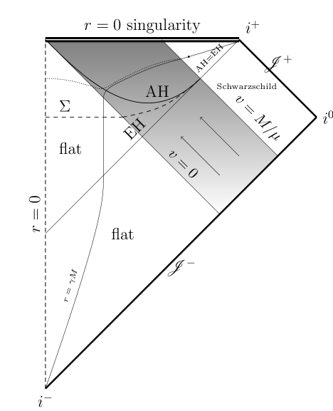
Figure 1: Conformal diagram of spacetime (3) with (6). The discontinuous line marked as $r=0$ is the origin of coordinates. A dressed curvature singularity is present at $r=0,\,v>0$. This is a spacelike future singularity. The spacetime is initially flat until null radiation flows in spherically from past infinity starting at $v=0$. The shaded region is a pure self-similar Vaidya spacetime. The spacetime becomes Schwarzschild with mass $M$ for all $v>M/\mu$. The apparent 3-horizon AH is spacelike in the shaded Vaidya region and then merges with EH at the 2-sphere $v=M/\mu$, $r=2M$. Notice that EH starts developing in the flat region. The portion above EH but below $v=0$ is a causal diamond in flat spacetime —the intersection of two light cones— and therefore it can de drawn without conformal distortion. A f-trapped closed surface entering the flat region is explicitly constructed in the main text. In the diagram it is represented by the dotted line, with a final portion within the $r=\gamma M$ hypersurface, with $\gamma<0.68514$. Nevertheless, f-trapped closed surfaces cannot extend below the hypersurface $\Sigma$ represented by the dashed line, and they all must have a non-empty portion above the AH, as it is explained in the main text.

These conditions imply in turn a restriction on the growth of the mass function BS :

$$\mu=\frac{1}{\gamma b}>\frac{1}{\gamma}\frac{b}{4a}>\frac{1}{4\gamma},\hskip 28.45274pt\gamma<0.68514.$$

It should be remarked that this construction of an explicit f-trapped closed surface is not optimal in the given Vaidya spacetime, so that there may well be examples for smaller values of $\mu$. However, from the restrictions that we will impose later by means of the hypersurface $\Sigma$ —see the next section—, f-trapped closed surfaces can never penetrate the flat region if $\mu\leq 1/8$.

The following conclusions are drawn from these results: (i) closed f-trapped surfaces can penetrate flat spacetime regions if the mass function rises fast enough; (ii) the dynamical horizon AH is not the sought for boundary $\mathscr{B}$ in general; and (iii) the teleological character of the EH translates into a non-local property of closed trapped surfaces, for they can have portions in a region of spacetime whose whole past is flat as long as some energy crosses them elsewhere to make their compactness feasible.

3 Fundamental general results

The main results leading to a better localization of the boundary $\mathscr{B}$ come from the interplay between (generalized) symmetries and generically trapped surfaces. They are fully general and based on ideas presented in MS ; S1 ; S2 ; S3 .

We start with the identity $({\pounds}_{\vec{\xi}}g)_{\mu\nu}=\nabla_{\mu}\xi_{\nu}+\nabla_{\nu}\xi_{\mu}$ for arbitrary vector fields $\vec{\xi}$, where ${\pounds}_{\vec{\xi}}$ denotes the Lie derivative with respect to $\vec{\xi}$. Projecting to $S$ and using (2)

$$({\pounds}_{\vec{\xi}}g|_{S})_{\mu\nu}\,e^{\mu}_{A}e^{\nu}_{B}=\overline{\nabla}_{A}\overline{\xi}_{B}+\overline{\nabla}_{B}\overline{\xi}_{A}+2\xi_{\mu}|_{S}K^{\mu}_{AB}\,.$$

Contracting now with $\gamma^{AB}$ we get the main formula to be exploited repeatedly in what follows

$$\framebox{$\displaystyle{\frac{1}{2}P^{\mu\nu}({\pounds}_{\vec{\xi}}g|_{S})_{\mu\nu}=\overline{\nabla}_{C}\overline{\xi}^{C}+\xi_{\rho}H^{\rho}}$}$$ (7)

where

$$P^{\mu\nu}\equiv\gamma^{AB}e^{\mu}_{A}e^{\nu}_{B}$$

is the orthogonal projector of $S$ —it projects to the part tangent to $S$.

This elementary formula (7) is very useful. Observe, for instance, that if $S$ is compact without boundary

$$\oint_{S}\xi_{\rho}H^{\rho}=\frac{1}{2}\oint_{S}P^{\mu\nu}({\pounds}_{\vec{\xi}}g|_{S})_{\mu\nu}$$

so that the sign of $\xi_{\rho}H^{\rho}$ is related to the sign of the projection to $S$ of the deformation $({\pounds}_{\vec{\xi}}g)_{\mu\nu}$. Thus,

if $\vec{\xi}$ is future-pointing on a region $\mathscr{R}\subset{\cal V}$, then the closed $S$ cannot be contained in $\mathscr{R}$ and generically f-trapped if $\oint_{S}P^{\mu\nu}({\pounds}_{\vec{\xi}}g|_{S})_{\mu\nu}\geq 0$.

The only exception is the case where $S$ is (partly) marginally f-trapped, $\vec{\xi}|_{S}$ is null and proportional to $\vec{H}$ and $P^{\mu\nu}({\pounds}_{\vec{\xi}}g|_{S})_{\mu\nu}=0$.

This general conclusion is applicable, for example, to conformal Killing vectors Exact (including the homothetic and proper Killing vectors) and to Kerr-Schild vector fields CHS . The former satisfy

$$({\pounds}_{\vec{\xi}}g)_{\mu\nu}=2\psi g_{\mu\nu}$$ (8)

for some function $\psi$, so that $P^{\mu\nu}({\pounds}_{\vec{\xi}}g|_{S})_{\mu\nu}=4\psi|_{S}$. Thus, the condition used in the reasoning above reduces to simply $\oint_{S}\psi\geq 0$. The Kerr-Schild vector fields are defined by

$$({\pounds}_{\vec{\xi}}g)_{\mu\nu}=2h\ell_{\mu}\ell_{\nu},\hskip 28.45274pt({\pounds}_{\vec{\xi}}\ell)_{\mu}=b\ell_{\mu}$$ (9)

for some functions $h$ and $b$, where $\ell_{\mu}$ is a fixed null one-form field ($\ell_{\mu}\ell^{\mu}=0$). Therefore $P^{\mu\nu}({\pounds}_{\vec{\xi}}g|_{S})_{\mu\nu}=2h\,\bar{\ell}_{A}\bar{\ell}^{A}$ and the condition holds if $h|_{S}\geq 0$.

Consider now the case where $\vec{\xi}$ is hypersurface orthogonal

$$\xi_{[\mu}\nabla_{\nu}\xi_{\rho]}=0\hskip 5.69054pt\Longleftrightarrow\hskip 5.69054pt\xi_{\mu}=-F\partial_{\mu}\tau$$

for some local functions $F>0$ and $\tau$. The hypersurfaces $\tau=$const. are called the level hypersurfaces and they are orthogonal to $\vec{\xi}$.

Assume again that $\vec{\xi}$ is future-pointing on $\mathscr{R}\subset{\cal V}$, then any minimal or generically f-trapped surface $S$ cannot have a local minimum of $\tau$ at any point $q\in\mathscr{R}$ such that $P^{\mu\nu}({\pounds}_{\vec{\xi}}g)_{\mu\nu}|_{q}\geq 0$.

This follows because at any local minimum $\bar{\xi}_{A}|_{q}=0$ from where one can derive using the main formula (7)

$$\left.\bar{F}\gamma^{AB}\frac{\partial^{2}\bar{\tau}}{\partial\lambda^{A}\partial\lambda^{B}}\right|_{q}=\left.-\frac{1}{2}P^{\mu\nu}({\pounds}_{\vec{\xi}}g)_{\mu\nu}\right|_{q}+\left.\xi_{\rho}H^{\rho}\right|_{q}$$

so that $\partial^{2}\bar{\tau}/\partial\lambda^{A}\partial\lambda^{B}|_{q}$ cannot be positive (semi)-definite. A detailed complete proof is given in BS1 .

Some important remarks are in order here: first of all, observe that $S$ does not need to be compact, nor fully contained in $\mathscr{R}$. Letting aside the exceptional possibility of minimal surfaces contained in a $\tau=$constant hypersurface if they have $P^{\mu\nu}({\pounds}_{\vec{\xi}}g)_{\mu\nu}|_{S}=0$, this result implies that, under the stated conditions, one can always follow a connected path along $S\cap\mathscr{R}$ with decreasing $\tau$. Note, also, that the result applies in particular but not only to (i) static Killing vectors, (ii) hypersurface-orthogonal causal conformal Killing vectors (8) with $\psi\geq 0$, and (iii) hypersurface-orthogonal causal Kerr-Schild vector fields (9) with $h\geq 0$.

Finally, consider the possibility of surfaces, compact or not, contained in one of the level hypersurfaces $\tau=$constant in $\mathscr{R}$. In that case, $\bar{\xi}_{A}=0$ all over $S\cap\mathscr{R}$ hence (7) implies

$$2\xi_{\rho}H^{\rho}=P^{\mu\nu}({\pounds}_{\vec{\xi}}g|_{S})_{\mu\nu}.$$

Thus, at any point $x\in S$ such that $P^{\mu\nu}({\pounds}_{\vec{\xi}}g)_{\mu\nu}|_{x}\geq 0$, $\vec{H}|_{x}$ cannot be timelike future-pointing, and it can be future-pointing null or zero only if $P^{\mu\nu}({\pounds}_{\vec{\xi}}g)_{\mu\nu}|_{x}=\xi_{\mu}H^{\mu}|_{x}=0$.

3.1 Application to the Vaidya imploding spacetime

The Vaidya spacetime (3) has a proper Kerr-Schild vector field of type (9) relative to the null direction $\vec{\ell}$ given by $\vec{\xi}=\partial_{v}$ CHS , because

$$({\pounds}_{\vec{\xi}}g)_{\mu\nu}=2\frac{dm}{dv}\ell_{\mu}\ell_{\nu}\,,\hskip 28.45274pt({\pounds}_{\vec{\xi}}\ell)_{\mu}=0$$

so that the function $h$ in (9) is $h=dm/dv\geq 0$. Note that $\vec{\xi}$ is hypersurface orthogonal, with the level function $\tau$ given by

$$\xi_{\mu}dx^{\mu}=-Fd\tau=dr-\left(1-\frac{2m(v)}{r}\right)dv$$ (10)

Concerning the causal character of $\vec{\xi}$, notice that

$$\xi_{\mu}\xi^{\mu}=-\left(1-\frac{2m(v)}{r}\right),\hskip 28.45274pt\ell_{\mu}\xi^{\mu}=-1$$

so that $\vec{\xi}$ is future pointing on the region $\mathscr{R}=\mathscr{R}_{0}\cup\mbox{AH}$, with $\mathscr{R}_{0}:\hskip 5.69054ptr>2m(v)$, timelike on $\mathscr{R}_{0}$ and null at the AH.

Hence, the results in this section are applicable to $\vec{\xi}$:

If the Vaidya spacetime (3) satisfies (4) and (5), then no closed generically f-trapped surface $S$ can be fully contained in the region $\mathscr{R}_{0}$. And the only ones contained in the region $\mathscr{R}:\,\,r\geq 2m(v)$ are the marginally f-trapped 2-spheres foliating the AH.

Standard results HE ; Wald imply that no generically f-trapped closed surface can penetrate outside the EH. Given that EH is the past Cauchy horizon HE ; S ; Wald of AH, EH=$H^{-}(\mbox{AH})$, the following conclusion follows:

no closed generically f-trapped surface can be fully contained in the region $D^{-}(\mbox{AH})$, so that they must penetrate the region $J^{+}(\mbox{AH})$ (given by $r\leq 2m(v)$.)

This agrees with theorem 4.1 in AG .

With regard to the boundary $\mathscr{B}$, we already know that closed trapped surfaces cross AH, and that the portion of EH within the flat region cannot be part of $\mathscr{B}$. But one can do even better and provide further restrictions on the location of $\mathscr{B}$. Put

$$\tau_{\Sigma}\equiv\inf_{x\in AH}\tau|_{x}\,.$$

It should be observed that $\tau_{\Sigma}$ is the least upper bound of $\tau$ on EH. The hypersurfaces $\tau=\tau_{c}$ are spacelike everywhere (and approaching $i^{0}$) if $\tau_{c}<\tau_{\Sigma}$, while they are partly spacelike and partly timelike, becoming null at AH, if $\tau_{c}>\tau_{\Sigma}$. The location of the spherically symmetric hypersurface $\Sigma$ depends on whether $\frac{dm}{dv}(0)>1/8$ or not. In the former case, $\Sigma$ does enter into the flat region. It may not be so in the other cases. $\Sigma$ is shown in figure 1 for the particular case with (6) and $\mu>1/8$. Notice that a characterization of $\Sigma$ is: the last hypersurface orthogonal to $\vec{\xi}$ which is non-timelike everywhere.

$\Sigma$ is a relevant spacetime object because:

No closed generically f-trapped surface penetrates the region with $\tau<\tau_{\Sigma}$.

The proof of this result uses the fact that the closed set above EH and below $\Sigma$ is contained in the region $\mathscr{R}$ where $\vec{\xi}$ is future pointing so that any compact $S$ entering there will reach a minimum. But then one checks that this minimum should be local BD ; BS . The results of this section imply then that $S$ cannot be generically f-trapped.

The hypersurface $\Sigma$ is a past limit for f-trapped closed surfaces. In fact, they cannot even touch $\Sigma$, as follows from the fact that $\tau$ is decreasing along a connected path in $S$. Thus, finally we deduce that

all f-trapped closed surfaces lie in $\tau>\tau_{\Sigma}$ and have points with $r<2m(v)$.

Thus, $\mathscr{B}\subset\{\tau\geq\tau_{\Sigma}\}\cap\{r\geq 2m(v)\}$.

4 The general spherically imploding spacetime

The previous results can be generalized to the general imploding spherically symmetric spacetime with an asymptotically flat end. The line-element can be written as

$$ds^{2}=-e^{2\beta}\left(1-\frac{2m(v,r)}{r}\right)dv^{2}+2e^{\beta}dvdr+r^{2}d\Omega^{2}$$ (11)

where now $\beta(v,r)$ and the mass function $m(v,r)$ depend on $r$ and the null advanced time $v$. The spherically symmetric apparent 3-horizon AH is a marginally trapped tube defined by

$$\mbox{AH}:\hskip 28.45274ptr-2m(r,v)=0\,.$$

AH is spacelike, null or timelike according to whether $\left.\frac{\partial m}{\partial v}\left(1-2\frac{\partial m}{\partial r}\right)\right|_{AH}$ is positive, zero or negative. As before, let us define the region where the round 2-spheres are untrapped $\mathscr{R}_{0}:\,\,r-2m(v,r)>0$.

Assume that the total mass function is finite and that there is an initial flat region:

$$m(v,r)=0\hskip 8.53581pt\forall v<0;\hskip 28.45274pt\forall v>0\,\left\{\begin{array}[]{c}0\leq m(v,r)\leq M<\infty\\ m(v,r)\not\equiv 0\end{array}\right..$$

Then there is a regular $\mathscr{J}^{+}$ and associated event horizon EH D . $\mbox{AH}_{1}$ denotes the connected component of AH associated to this EH. It separates the region $\mathscr{R}_{1}$, defined as the connected subset of $\mathscr{R}_{0}$ containing the flat portion, from a region containing f-trapped 2-spheres. The dominant energy condition is also assumed, and furthermore the matter-energy is incoming so that $\partial m/\partial v\geq 0$ on $(\mathscr{R}_{1}\cup\mbox{AH}_{1})\cap J^{+}(EH)$. Under these assumptions, $\mbox{AH}_{1}$ will eventually be spacelike (actually achronal) and asymptotic to (probably merging) the EH Wil . The relevant Penrose diagrams are shown in figure 2.

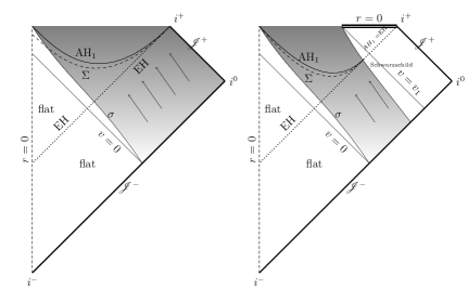
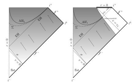
Figure 2: Conformal diagrams of (11) for the cases with $m(v,r)<M$ everywhere (first and third) or with $m(v,r)=M$ in some open asymptotic region (second and fourth). The spacetime is flat below $v=0$. EH may start developing in the flat region or not. The hypersurface $\sigma$ separating the flat portion and the rest of the spacetime cannot be spacelike. The shaded regions have non-vanishing energy-momentum. The connected component $\mbox{AH}_{1}$ approaches EH either asymptotically or at some finite value of $v\leq v_{1}$ and $r=2M$. The first collapsing shell $\sigma$ may lead or not to the formation of a singularity depending on the properties of the mass function $m(v,r)$. The future evolution of the spacetime is thus left open for the shaded regions, and the third and fourth diagrams describe cases where there is a regular centre of symmetry in the non-flat non-empty region. $\mbox{AH}_{1}$ is spacelike when approaching EH, but this is not necessarily so in other regions: in the last two diagrams, $\mbox{AH}_{1}$ is timelike close to the left upper corner. The hypersurface $\Sigma$ puts a limit to the past on the possible location of f-trapped closed surfaces and, therefore, of $\mathscr{B}$. This hypersurface may enter the flat region (an example is the first diagram) or not. If the inflow of mass stops and there is a final Schwarzschild region of mass $M$, then $\Sigma$ merges with the EH and $\mbox{AH}_{1}$ at $r=2M$ (second and fourth diagrams). The diagrams shown are only relevant possibilities, and many other possible combinations of the mentioned features are also feasible.

4.1 The hypersurface $\Sigma$

The spacetime (11) does not have a Kerr-Schild vector field in general, but we can insist on using $\vec{\xi}=\partial_{v}$, called the Kodama vector Ko . This is hypersurface orthogonal with the level function $\tau$ defined by

$$\xi_{\mu}dx^{\mu}=-Fd\tau=e^{\beta}dr-e^{2\beta}\left(1-\frac{2m(v,r)}{r}\right)dv.$$ (12)

Its norm is

$$\xi_{\mu}\xi^{\mu}=-e^{2\beta}\left(1-\frac{2m(v,r)}{r}\right),\hskip 28.45274pt\ell_{\mu}\xi^{\mu}=-1$$

where now $\ell_{\mu}dx^{\mu}=-e^{\beta}dv$, $\vec{\ell}=-e^{-\beta}\partial_{r}$, so that $\vec{\xi}$ is future-pointing timelike (null) on $\mathscr{R}_{0}$ (at AH).

As in the Vaidya case, set $\tau_{\Sigma}\equiv\inf_{x\in AH_{1}}\tau|_{x}$ and define $\Sigma\equiv\{\tau=\tau_{\Sigma}\}$. The properties and characterization of $\Sigma$ are the same as in the Vaidya case. Concerning its location, this depends on whether $8\dot{m}_{0}>(1-2m^{\prime}_{0})^{2}$ or not. Here $\dot{m}_{0}$ and $m^{\prime}_{0}$ are the limits of $\frac{\partial m}{\partial v}$ and $\frac{\partial m}{\partial r}$ when approaching $(v=v_{0}^{+},r=0)$, respectively, $v_{0}\geq 0$ being the value of $v|_{\sigma}$ at $r=0$ (see figure 2). In the former case, $\Sigma$ does penetrate the flat region, but it may not be so in the other cases BS1 . Some possibilities have been shown in figure 2.

The Lie derivative of the metric with respect to the Kodama vector can be easily computed

$$({\pounds}_{\vec{\xi}}g)_{\mu\nu}=e^{2\beta}\frac{2}{r}\frac{\partial m}{\partial v}\ell_{\mu}\ell_{\nu}-\frac{\partial\beta}{\partial v}\left(\ell_{\mu}\xi_{\nu}+\ell_{\nu}\xi_{\mu}\right)$$

and this can be seen to be sufficient so that the fundamental results —concerning the non-existence of a minimum of $\tau$ and related— hold. Therefore, one can obtain the following important results:

• No closed generically f-trapped surface can penetrate the region $\tau<\tau_{\Sigma}$.

• No closed f-trapped surface can enter the region $\tau\leq\tau_{\Sigma}$.

• The minimum $\tau_{m}$ of $\tau$ on a closed f-trapped $S$ is always attained within $r\leq 2m(v)$,

• furthermore, is $S$ happens to cross $\mbox{AH}_{1}$, then $\tau|_{S\cap\mathscr{R}_{1}}>\hat{\tau}_{m}>\tau_{m}$ and $r|_{S\cap\mathscr{R}_{1}}<\hat{r}$ where $\hat{\tau}_{m}$ is the minimum value of $\tau|_{S}$ on $\mbox{AH}_{1}$, and $\hat{r}$ is the value of $r$ at the 2-sphere $\hat{\varsigma}\equiv\{\tau=\hat{\tau}_{m}\}\cap\mbox{AH}_{1}$.

As before, these properties of $\Sigma$ provide strong restrictions on the possible locations of the boundary $\mathscr{B}$. This is analyzed in more detail in the next section.

5 The boundary $\mathscr{B}$ in spherical symmetry

Start by defining Hay ; BS1 the future-trapped region $\mathscr{T}$ as the set of points $x\in{\cal V}$ such that $x$ lies on a closed f-trapped surface. $\mathscr{T}$ is an open set, as follows from the application of the formula for the variation of the null expansions (e.g. AMS or many of references therein). However, $\mathscr{T}$ is not necessarily connected.

Denote then by $\mathscr{B}$ the boundary of the f-trapped region: $\mathscr{B}\equiv\partial\mathscr{T}$. This is related to the “trapping boundaries” in Hay . $\mathscr{B}$ being the boundary of an open set, it is a closed set without boundary. Moreover $\mathscr{B}\cap\mathscr{T}=\emptyset$. Observe that $\mathscr{B}$ divides the spacetime in two separate portions, because $\mathscr{B}$ is also the boundary of the untrapped region defined by the set of points $x\notin\mathscr{T}$. Again, $\mathscr{B}$ is not necessarily connected. The connected component of $\mathscr{B}$ associated to $\mbox{AH}_{1}$ will be denoted by $\mathscr{B}_{1}$. It is important to remark that $\mathscr{B}$ is a genuine spacetime object, independent of any foliations or initial Cauchy data sets. Hence, $\mathscr{B}$ is basically different from the boundary of f-trapped surfaces contained in given slices and studied, e.g., in AM .

The previous properties are independent of spherical symmetry. If this symmetry is assumed, then one has:

in arbitrary spherically symmetric spacetimes, $\mathscr{T}$ and $\mathscr{B}$ have spherical symmetry. Actually, $\mathscr{B}$ (if not empty) is a spherically symmetric hypersurface without boundary.

Set $\tau_{\mathscr{B}}\equiv\inf_{x\in\mathscr{B}}\tau|_{x}$ where $\tau=$const. are the level hypersurfaces of the Kodama vector $\vec{\xi}$. The following important results hold BS1 :

• The connected component $\mathscr{B}_{1}$ does not have a positive minimum value of $r$,

• moreover $\tau_{\mathscr{B}}=\inf_{x\in\mathscr{B}_{1}}\tau|_{x}=\tau_{\Sigma}$,

• $\mathscr{B}_{1}\subset(\mathscr{R}_{1}\cup\mbox{AH}_{1})\cap\{\tau\geq\tau_{\Sigma}\}$,

• $\mathscr{B}_{1}$ merges with, or approaches asymptotically, $\Sigma$, $\mbox{AH}_{1}$ and EH in such a way that $(\mathscr{B}_{1}\backslash EH)\cap\mbox{AH}_{1}=\emptyset$.

• $\mathscr{B}_{1}\backslash$EH cannot be tangent to a $\tau=$const. hypersurface, so that $\tau$ is a monotonically decreasing function of $r$ on $\mathscr{B}_{1}\backslash$EH.

• In particular, $\mathscr{B}_{1}\cap(\Sigma\backslash EH)=\emptyset$.

• $\mathscr{B}_{1}$ cannot be non-spacelike everywhere. And it is spacelike close to the merging with $\Sigma$ and EH.

These results prove that $\mathscr{B}_{1}\backslash EH$ must be placed strictly above $\Sigma$ and strictly below $\mbox{AH}_{1}$. The allowed region for $\mathscr{B}_{1}$ is shown in figure 3 for several possibilities of interest.

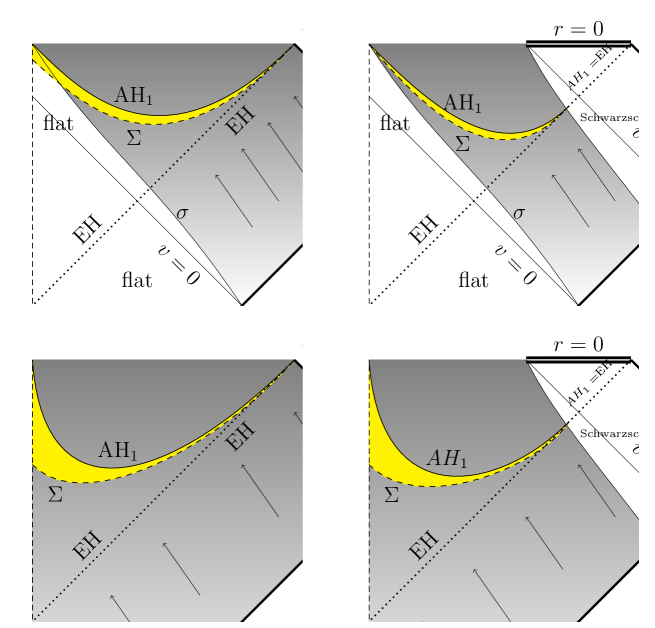
Figure 3: These are enlargements of appropriate regions for the four cases shown in figure 2. The boundary $\mathscr{B}_{1}$ must lie in the yellow region, and it cannot touch its upper and lower limit —given by $\mbox{AH}_{1}$ and $\Sigma$— away from EH. If there is a Schwarzschild region with mass $M$ then $\mathscr{B}_{1}$ coincides with EH (and $\Sigma$ and $\mbox{AH}_{1}$) there.

Observe that $(\mathscr{B}_{1}\backslash EH)$ is entirely contained in the region $\mathscr{R}_{1}$, that is to say, in the region with $r>2m$ so that $\vec{\xi}$ is timelike and future-pointing there. Given that, from the fundamental results, no generically f-trapped closed surface can be contained in that region, it follows that

$(\mathscr{B}_{1}\backslash EH)$ cannot be a marginally trapped tube, let alone a dynamical or future outer trapping horizon.

Notice that the only closed marginally f-trapped surfaces that can be contained in $\mathscr{B}_{1}$ are those which are actually on its part $\mathscr{B}_{1}\cap$EH, if any. Observe also that this result implies that the notion of “limit section” in Hay is generically non-existent, and thus theorem 7 in that reference is essentially empty in the sense that its assumptions are rarely met.

Let

$$\vec{\eta}=\partial_{v}+e^{\beta}A\partial_{r}$$

be the normal vector field to $\mathscr{B}_{1}$ and extend $A$ to be a function $A(v,r)$ on a neighborhood of $\mathscr{B}_{1}$, so that $\mathscr{B}_{1}$ belongs to a local foliation of hypersurfaces $\Sigma_{t}\equiv\{t=\mbox{const.}\}$, where $t$ is defined by ($G>0$)

$$\eta_{\mu}dx^{\mu}=-Gdt=e^{\beta}dr-e^{2\beta}\left(1-\frac{2m}{r}-A\right)dv.$$ (13)

By applying the reasonings used to derive the fundamental results to this hypersurface-orthogonal vector field on the regions $\mathscr{B}^{s}_{1}$ where it is spacelike —for instance at the asymptotic region when $\mathscr{B}_{1}$ is about to merge with $\Sigma$ and $\mbox{AH}_{1}$—, one can deduce that

$$P^{\mu\nu}({\pounds}_{\vec{\eta}}g)_{\mu\nu}|_{\mathscr{B}^{s}_{1}}\leq 0$$ (14)

for all projectors of generically f-trapped surfaces tangent to $\mathscr{B}_{1}^{s}$ at some point. This puts severe restrictions on the boundary $\mathscr{B}_{1}$, see BS1 . In particular,

$\mathscr{B}_{1}$ cannot have a positive semi-definite second fundamental form at any point where it is spacelike.

Actually, the condition (14) is much more restrictive than this because it has to hold for all mentioned projectors. The combination of this with the spherical symmetry leads in turn to severe restrictions on the second fundamental form of $\mathscr{B}^{s}_{1}$ —more generally, on the projection of ${\pounds}_{\vec{\eta}}g$ to $\mathscr{B}_{1}$, be this spacelike or not— and its eigenvalues. This is work in progress BS1 .

6 Conclusions and outlook

The main conclusions are:

• Closed trapped surfaces can penetrate flat portions of spacetime.

• Closed trapped surfaces are highly non-local, a manifestation of the teleological character of the event horizon.

• The boundary $\mathscr{B}$ seems to be a fundamental spacetime object, specially in asymptotically flat black-hole spacetimes. It defines the region where dynamical or future outer trapping horizons can exist.

• $\mathscr{B}\backslash$EH does not include any portion of a marginally trapped tube. Actually, it does not contain any closed generically f-trapped surface.

• The location of $\mathscr{B}$ has been severely restricted, and we are working on its intrinsic characterization.

• Of course, one wishes to eventually give up spherical symmetry. In this sense

  • The techniques used to define $\tau$ and to utilize it are completely general.

  • The main formula (7), the general results on minima, etc. are also fully general.

References

- (1) L. Andersson, M. Mars and W. Simon, Phys. Rev. Lett. 95, 111102 (2005)
- (2) L. Andersson, M. Mars and W. Simon, Adv. Theor. Math. Phys. 12 853 (2008)
- (3) L. Andersson and J. Metzger, The area of horizons and the trapped region, preprint arXiv:0708.4252
- (4) A. Ashtekar and B. Krishnan, Living Rev. Relativity 7 10 (2004)
- (5) A. Ashtekar and G.. J. Galloway, Adv. Theor. Math. Phys. 9 1 (2005)
- (6) I. Ben-Dov, Phys.Rev. D 75 (2007) 064007
- (7) I. Bengtsson and J.M.M. Senovilla, A note on trapped surfaces in the Vaidya solution, preprint arXiv:0809.2213
- (8) I. Bengtsson and J.M.M. Senovilla, The boundary of the region with trapped surfaces in spherical symmetry, in preparation
- (9) I. Booth, Can. J. Phys. 83 1073 (2005)
- (10) B. Coll, S.R. Hildebrandt and J.M.M. Senovilla, Gen. Rel. Grav. 33, 649 (2001).
- (11) M. Dafermos, Class. Quantum Grav. 22, 2221 (2005)
- (12) D.M. Eardley, Phys. Rev. D 57, 2299 (1998)
- (13) S.W. Hawking, Commun. Math. Phys. 25 152 (1972).
- (14) S.W. Hawking, G.F.R. Ellis, The large scale structure of space-time, (Cambridge Univ. Press, Cambridge, 1973).
- (15) S.A. Hayward, Phys. Rev. D 49, 6467 (1994)
- (16) S.A. Hayward, Class. Quantum Grav. 11, 3025 (1994)
- (17) W.A. Hiscock, L.G. Williams and D.M. Eardley, Phys. Rev. D 26, 751 (1982)
- (18) H Kodama, Prog. Theor. Phys. 63 1217 (1980)
- (19) M. Kriele, Spacetime, (Springer, Berlin, 1999).
- (20) M. Kriele and S.A. Hayward, J. Math. Phys. 38, 1593 (1997)
- (21) B. Krishnan, Class. Quantum Grav. 25 114005 (2008)
- (22) Y. Kuroda, Prog. Theor. Phys. 72 63 (1984)
- (23) M. Mars and J.M.M. Senovilla, Class. Quantum Grav. 20 (2003) L293.
- (24) B. O’Neill, Semi-Riemannian Geometry: With Applications to Relativity (Academic Press, 1983).
- (25) R. P. A. C. Newman, Class. Quantum Grav. 4, 277 (1987)
- (26) A. Papapetrou, Formation of a singularity and causality, in A random walk in relativity and cosmology, N. Dadhich et al. (eds.), (Wiley, 1985)
- (27) E. Schnetter and B. Krishnan, Phys. Rev. D 73, 021502(R) (2006)
- (28) J.M.M. Senovilla, Gen. Rel. Grav. 30, 701 (1998).
- (29) J.M.M. Senovilla, Class. Quantum Grav. 19, L113 (2002).
- (30) J.M.M. Senovilla, Novel results on trapped surfaces, in “Mathematics of Gravitation II”, (Warsaw, September 1-9, A Królak and K Borkowski eds, 2003); http://www.impan.gov.pl/Gravitation/ConfProc/index.html (gr-qc/03011005).
- (31) J.M.M. Senovilla, J. High Energy Physics 11 (2003) 046.
- (32) J.M.M. Senovilla, Class. Quantum Grav. 24 (2007) 3091-3124
- (33) Stephani H, Kramer D, MacCallum M A H, Hoenselaers C and Herlt E Exact Solutions to Einstein’s Field Equations Second Edition (Cambridge University Press, Cambridge, 2003)
- (34) P.C. Vaidya, Proc. indian Acad. Soc. A 33 264 (1951)
- (35) Wald, R M 1984 General Relativity (The University of Chicago Press, Chicago)
- (36) C. Williams, “Asymptotic Behavior of Spherically Symmetric Marginally Trapped Tubes”, preprint, arXiv:gr-qc/0702101