The basic role of magnetic field in stellar evolution

Abstract

Magnetic field is playing an important role at all stages of star evolution from star formation to the endpoints. The main effects are briefly reviewed. We also show that O–type stars have large convective envelopes, where convective dynamo could work. There, fields in magnetostatic balance have intensities of the order of 100 G.

A few OB stars with strong polar fields ([Henrichs et al. (2003a), Henrichs et al. 2003a]) show large N–enhancements indicating a strong internal mixing. We suggest that the meridional circulation enhanced by an internal rotation law close to uniform in these magnetic stars is responsible for the observed mixing. Thus, it is not the magnetic field itself which makes the mixing, but the strong thermal instability associated to solid body rotation.

A critical question for evolution is whether a dynamo is at work in radiative zones of rotating stars. The Tayler-Spruit (TS) dynamo is the best candidate. We derive some basic relations for dynamos in radiative layers. Evolutionary models with TS dynamo show important effects: internal rotation coupling and enhanced mixing, all model outputs being affected.

1 Introduction

The magnetic field of a star is, like the scent of a flower, subtle and invisible, but it plays an essential role in evolution. Magnetic field is often not accounted for in star models. However, the examples below show that from star formation to the endpoints as compact objects, magnetic fields and rotation strongly influence the course of evolution and all model outputs.

In Sect. 2, we give an overview where in evolution the fields are intervening. In Sect. 3, we emphasize some critical observations. In Sect. 4, we focus on the general dynamo equations, with examples in Sect. 5 and 6 for the Tayler–Spruit (TS) dynamo.

2 Overview on the magnetic field in star formation and evolution

Fig. 1 shows the evolutionary track of the Sun from its formation to its endpoint with indications of the various effects of the magnetic field coming into play.

–1. Collapse and ambipolar diffusion: magnetic field may contribute to cloud support. For contraction to occur it is necessary that the energy density of magnetic field $u_{\mathrm{B}}={B^{2}}/({8\;\pi})$ is smaller than the density of gravitational energy $u_{\mathrm{G}}=\frac{3}{5}\,\frac{GM^{2}}{R\;(\frac{4}{3}\pi R^{3})}\;=\;\frac{9}{20\,\pi}\;\frac{GM^{2}}{R^{4}}$. This defines a critical mass $M_{\mathrm{B}}$ above which gravitation dominates,

$$M_{\mathrm{B}}\approx\left(\frac{5}{18\,\pi^{2}}\right)^{\frac{1}{2}}\frac{\Phi}{\sqrt{G}}\;=\;0.17\,\frac{\Phi}{\sqrt{G}}\;,$$ (1)

with the magnetic flux $\Phi=\pi\,B\,R^{2}$. In the original derivation ([Mouschovias & Spitzer 1976, Mouschovias & Spitzer 1976]), a numerical factor 0.13 was obtained instead of 0.17 in this simple derivation. If $M\,>\,M_{\mathrm{B}}$, large clusters or associations form. If $M\,<\,M_{\mathrm{B}}$, no contraction occurs until the small ionized fraction ($\sim 10^{-7}$) to which the field is attached has diffused (in about $10^{7}$ yr) out from the essentially neutral gas forming the cloud.

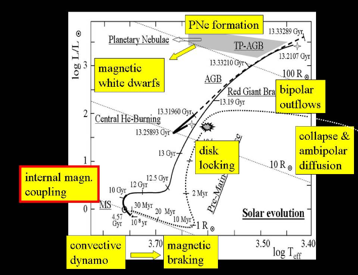
Figure 1: The evolutionary track of the Sun from the protostellar phase to the phase of planetary nebulae (courtesy from C. Charbonnel) with superposed indications of the various magnetic intervening processes

–2. Bipolar outflows: massive molecular outflows are often detected in region of star formation. A large fraction of the infalling material is not accreted by the central object but it is ejected in the polar directions. In massive stars, the ejection cones are relatively broad. Radiative heating and magnetic field are likely driving the outflows. Remarkably the mass outflow rates correlate with the luminosities of the central objects over 6 decades in luminosity, from about 1 L_⊙ to $10^{6}$ L_⊙, as shown by [Churchwell (1998), Churchwell (1998)] and [Henning et al. (2000), Henning et al. (2000)].

–3. Disk locking: from the dense molecular clouds to the present Sun, the specific angular momentum decreases by $\sim 10^{6}$. Among the processes reducing the angular momentum in stars, disk locking is a major one ([Hartmann 1998, Hartmann 1998]). Fields of $\sim 1$ kG are sufficient for the coupling between the star and a large accretion disk. The contracting star is bound to its disk and it keeps the same angular velocity during contraction, thus losing a lot of angular momentum. The typical disk lifetime is a few $10^{6}$ yr.

–4. Convective dynamos and magnetic braking: solar types stars have external convective zones which produce a dynamo. The resulting magnetic field creates a strong coupling between the star and the solar wind, which leads to losses of angular momentum. The relation expressing these losses as a function of the stellar parameters have been developed by [Kawaler 1988, Kawaler (1988)]. Further improvements to account for saturation effects and mass dependence have been brought ([Krishnamurti et al. 1997, Krishnamurti et al. 1997]).

Massive OB stars also have significant external convective zones which may represent up to 15% of the radius. Surprisingly rotation enhances these convective zones ([Maeder et al. 2008, Maeder et al. 2008]), which may also produce magnetic braking.

–5. Dynamo in radiative zones: is there a dynamo working in internal radiative zones? This is the biggest question concerning magnetic field and stellar evolution, with far reaching consequences concerning mixing of the chemical elements and losses of the angular momentum. This question is also essential regarding the rotation periods of pulsars and the origin of GRBs. We devote Sect. 4 to 6 to this question.

–6. Magnetic field in AGB stars, planetary nebulae and final stages: red giants, AGB stars and supergiants have convective envelopes and thus dynamos. Evidences of magnetic fields up to kG in some central stars of planetary nebulae are given (see Jordan, this meeting), they contribute to shaping the nebulae (see Blackman, this meeting). White dwarfs have magnetic fields from about $10^{4}$ up to $10^{9}$ G, the highest fields likely resulting from common envelope effects in cataclysmic variables.

3 Magnetic fields and abundances: the Henrichs et al. results

Since OB stars also have convective envelopes, the question arises what are the possible fields created by the associated dynamos. If one considers a flux tube in magnetostatic balance in the stellar atmosphere, the equilibrium field is given by the condition ${B^{2}}/({8\,\pi})\,=\,P_{\mathrm{ext}}-P_{\mathrm{int}}$. At optical depth $\tau=2/3$, the pressure is $P(\tau=2/3)\,\approx\,({2}/{3})\,{g}/{\kappa}$. Since $P_{\mathrm{int}}>0$, the maximum possible field $B_{\mathrm{eq}}$ for magnetic equilibrium is ([Safier 1999, Safier 1999])

$$B_{\mathrm{eq}}\left(\tau={2}/{3}\right)\,\approx\,\left(\frac{16\,\pi}{3}\,\frac{g}{\kappa}\right)^{1/2}\;.$$ (2)

Table 1: The equilibrium fields. The stars are on the ZAMS, except the Sun.

Spectral type	field	Spectral type	field
M0	2.8 kG	G0	1.0 kG
KO	1.5 KG	F2	0.6 kG
Sun	1.3 kG	*O9	0.2 kG
* from the author

Table 1 gives the corresponding estimates for stars of various types. The observed field intensities are often within a factor of 2 from the maximum values given in the table. Searches for magnetic fields in OB–type stars show no general evidence of fields above the level of $\sim$100 G ([Mathys 2004, Mathys 2004]). This is of the order of magnitude of the possible fields in magnetostatic equilibrium in the convective envelopes of OB stars. The strong fields of 1 kG or more are not widespread ([Hubrig et al. (2008), Hubrig et al. 2008]).

Noticeable exceptions were found and studied by Henrichs and colleagues ([Henrichs et al. (2003a), Henrichs et al. 2003a], [Henrichs et al. (2003b), Henrichs et al. 2003b]). Their remarkable finding is that the few stars with high polar fields $B_{\mathrm{p}}$ also show N and He enhancements together with C and O depletions, in particular for the 4 stars listed below.

Table 2: Stars with intense fields and N enrichments from ([Henrichs et al. (2003a), Henrichs, Neiner & Geers 2003a])

$\beta$ Cep	B1IVe	v $\sin i=$	27	km s-1	$B_{\mathrm{p}}$=360 G	$\Delta\log$ N=1.2
V2052 Oph	B1IVe	v $\sin i=$	63	km s-1	$B_{\mathrm{p}}$=250 G	$\Delta\log$ N=1.3
$\zeta$ Cas	B2IV	v $\sin i=$	17	km s-1	$B_{\mathrm{p}}$=340 G	$\Delta\log$ N=2.6
$\omega$ Ori	B2IVe	v $\sin i=$	172	km s-1	$B_{\mathrm{p}}$=530 G	$\Delta\log$ N=1.8

The abundances are given in Table LABEL:tblH as the difference in log between the observed N abundance and the solar values. These are typical signatures of CNO processing, which give strong evidences of internal mixing in stars with a high magnetic field. These few results bring a lot of interesting questions.

The law of isorotation of Ferraro clearly implies that an internal polar field enforces solid body rotation, see also Sect. 6. Now, the above results suggest that even in presence of uniform rotation, there is an efficient mixing. What is the mixing process in stars with a polar magnetic field? Shear turbulence is generally the main mixing process of chemical elements. However, it is absent here, since the stars rotate uniformly.

The only process among those usually acting in massive stars is meridional circulation. Is it sufficient to produce such a mixing? In differentially rotating stars, it is usually much less efficient than shear mixing for the transport of the chemical elements ([Meynet & Maeder 2000, Meynet & Maeder 2000]), while it is very efficient for the transport of angular momentum. However, we found that meridional circulation is strongly enhanced by solid body rotation, since uniform rotation creates a strong breakdown of radiative equilibrium.

In evolutionary models with magnetic field and meridional circulation, there is a strong interplay between meridional circulation and magnetic field ([Maeder & Meynet (2005), Maeder & Meynet 2005]):

• Differential rotation creates the magnetic field.

• Magnetic field tends to suppress differential rotation.

• A rotation close to uniform strongly enhances meridional circulation.

• Meridional circulation increases differential rotation and produces mixing.

• Differential rotation feeds the dynamo and magnetic field (the loop is closed).

As a result, the star reaches an equilibrium rotation law close to uniform (see models in the above ref.), with always a strong thermal instability amplifying meridional circulation and thus chemical mixing. Models show that the high enrichments in magnetic stars with a dynamo (Sect. 4) are essentially due to the transport by meridional circulation. Thus, it is not the magnetic field itself which makes the mixing, but the thermal instability associated to the solid rotation created by the field.

The high surface magnetic field of these stars, which likely have a significant mass loss, produces a strong magnetic braking, which implies that these stars will reach a rather low rotation velocities during their evolution. The braking would tend to produce some internal differential rotation. However, the magnetic coupling is certainly strong enough to maintain a rotation law close to uniform, as illustrated by the models.

4 Dynamos in radiative layers: general properties and equations

The major question concerning magnetic fields and stellar evolution is whether a dynamo operates in radiative zones of differentially rotating stars. A magnetic field has great consequences on the evolution of the rotation velocity by exerting an efficient torque able to impose a nearly uniform rotation. This influences all the model outputs (lifetimes, chemical abundances, tracks, chemical yields, supernova types) as well as the rotation in the final stages, white dwarfs, neutron stars or black holes.

Here we first examine some general equations implied by any dynamo. The particular properties of the Tayler–Spruit (TS) dynamo have been studied by [Spruit (2002), Spruit (2002)] and we are using many of the equations he derived. Spruit considered the radiative zones in two cases, –1) when the $\mu$–gradient dominates, and –2) when the $\mu$–gradient is negligible. The more general equations of the TS dynamo have been developed by ([Maeder & Meynet (2005), Maeder & Meynet 2005]). The TS dynamo is at present a debated subject. Some numerical simulations by [Braithwaite (2006), Braithwaite (2006)] and by [Zahn et al. (2007), Brun et al. (2007)] confirm the existence of Tayler’s instability. Braithwaite also finds the existence of a dynamo loop in agreement with Spruit’s analytical developments. However, Zahn et al. do not find the dynamo loop proposed by Spruit and question what may close the loop.

4.1 Energy conservation

If a dynamo is working in a differentially rotating radiative zone, it is governed by some general relations expressing the order of magnitude of its various properties. First, the rate of magnetic energy production $W_{\mathrm{B}}$ per unit of time and volume must be equal to the rate $W_{\nu}$ of dissipation of rotational energy by the magnetic viscosity $\nu$. We assume here that the whole energy dissipated is converted into magnetic energy. The differential motions are those of the shellular rotation with an angular velocity $\Omega(r)$, so that the velocity difference at radius $r$ is $dv=r\,d\Omega$. The amount of energy corresponding to a velocity difference $dv$ during a time $dt$ for an element of matter $dm$ in a volume $dV$ is

$$W_{\nu}=\frac{1}{2}\,dm\,(dv)^{2}\frac{1}{dV}\,\frac{1}{dt}=\frac{1}{2}{\varrho}\,\nu\left(\frac{dv}{dr}\right)^{2}={1\over 2}\varrho\nu\Omega^{2}q^{2}\quad\quad\mathrm{with}\quad q=r\left|\nabla\Omega\right|/\Omega,$$ (3)

because the viscous time $dt$ over $dr$ is given by $dt=(dr)^{2}/\nu$. The magnetic energy density is $u_{\mathrm{B}}={B^{2}}/(8\pi)$, it is produced within the characteristic growth time of the magnetic field $\sigma_{\mathrm{B}}^{-1}$, thus the rate $W_{\mathrm{B}}$ of magnetic energy creation by units of volume and time is

$$W_{\mathrm{B}}=\frac{B^{2}}{8\pi}\sigma_{\mathrm{B}}=\frac{1}{2}\omega^{2}_{\mathrm{A}}r^{2}\sigma_{\mathrm{B}}\varrho\;,$$ (4)

where we have used the expression of the Alfvén frequency $\omega_{\mathrm{A}}\,=\,\frac{B}{r(4\,\pi\varrho)^{1/2}}$. Now, let us assume $W_{\nu}=W_{\mathrm{B}}$, i.e. that the excess of energy in the differential rotation (compared to an average constant rotation) is converted to magnetic energy by unit of time. This gives the following expression for the viscosity coefficient of magnetic coupling

$$\nu=\frac{\omega^{2}_{\mathrm{A}}\,r^{2}\,\sigma_{\mathrm{B}}}{\Omega^{2}\,q^{2}}\;.$$ (5)

This is the coefficient which intervenes in the expression for the transport of angular momentum, in the Lagrangian form as given by Eq. (29) below. Let us note that compared to the energy available for the solar dynamo driven by convection, the amount of energy available from differential rotation is very limited.

4.2 The $\alpha$ and $\omega$–effects: vertical instability and stretching of the field lines

A dynamo needs both the $\alpha$–effect and $\omega$–effect. The $\alpha$–effect consists in the generation of a poloidal field component from the horizontal component. In the Sun, the $\alpha$–effect is created by the convective motions and by the twisting of the magnetic loop by the Coriolis force. However, other instabilities with a vertical component may produce the necessary $\alpha$–effect. The $\omega$–effect consists mainly of the stretching of a small radial field component in the East–West directions. The winding–up of the field lines generates a stronger horizontal field component, converting some kinetic energy into magnetic energy.

If due to an instability in radiative layers, some vertical displacements (necessary for the $\alpha$–effect) with an amplitude $l_{r}/2$ occur around an average stable position, the restoring buoyancy force produces vertical oscillations with a frequency equal to the Brunt–Va̋isa̋la̋ frequency $N$. The restoring oscillations will have an average density of kinetic energy $u_{\mathrm{N}}=f_{N}\,\rho\,\ell^{2}\,N^{2}$, where $f_{N}\sim 1$. In order to produce a vertical displacement, the magnetic field must overcome the buoyancy effect. In terms of energy densities, this is $u_{\mathrm{B}}>u_{\mathrm{N}}$, where $u_{\mathrm{B}}$ has been given in the previous section. Otherwise the restoring force of gravity would counteract the magnetic instability at the dynamical timescale. From this condition, one obtains $\ell^{2}<\frac{1}{2f_{\mathrm{N}}}\,r^{2}\,\frac{\omega^{2}_{\mathrm{A}}}{N^{2}}$. If, $f_{\mathrm{N}}={1\over 2}$, we have the condition ([Spruit (2002), Spruit 2002])

$$\ell<l_{r}=\;r\;\frac{\omega_{\mathrm{A}}}{N}\;,$$ (6)

where $r$ is the radius at the considered level in the star.

The stretching of the field lines for the $\omega$–effect is governed by the induction equation

$$\frac{\partial\vec{B}}{\partial t}=\vec{\nabla}\times(\vec{v}\times\vec{B})+\eta\,\nabla^{2}\vec{B}\;.$$ (7)

An unstable vertical displacement of size $\ell$ from the azimuthal field of lengthscale $r$ and intensity $B_{\varphi}$ also feeds a radial field component $B_{r}$. The relative sizes of these two field components are defined by the induction equation (7), which gives the following scaling over the time $\delta t$ characteristic of the unstable displacement,

$$B_{r}\,\approx\,\delta B\,\approx\,\frac{1}{r}\,\frac{\ell}{\delta t}\,B_{\varphi}\,\delta t\;.$$ (8)

For the maximum displacement $l_{r}$ given by Eq. 6, this gives

$$\frac{B_{r}}{B_{\varphi}}\approx\frac{l_{r}}{r}\;,$$ (9)

which provides ([Spruit (2002), Spruit 2002]) an estimate of the ratio of the radial to azimuthal fields.

4.3 The magnetic and thermal diffusivities

The magnetic diffusivity $\eta$ tends to damp the instability, while the thermal diffusivity $K$ produces heat losses from the unstable fluid elements and thus reduces the buoyancy forces opposed to the magnetic instability. Both effects have to be accounted for.

If the radial scale of the vertical instability is small, the perturbation is quickly damped by the magnetic diffusivity $\eta$ (in cm² s^-1). The radial amplitude must satisfy,

$$l_{r}^{2}>\frac{\eta}{\sigma_{\mathrm{B}}}\;,$$ (10)

where, as seen above, $\sigma_{\mathrm{B}}$ is the characteristic frequency for the growth of the instability. The combination of the two limits (9) and (10) gives for the case of marginal stability,

$$\eta\,=\,\frac{r^{2}\,\omega^{2}_{\mathrm{A}}\,\sigma_{\mathrm{B}}}{N^{2}}\;.$$ (11)

For given $\eta$ and $\sigma_{\mathrm{B}}$, this provides the minimum value of $\omega_{\mathrm{A}}$, and thus of the magnetic field $B$, for the instability to occur. The instability is confined within a domain, limited on the large side by the stable stratification (6) and on the small scales by magnetic diffusion (10). For the case of marginal stability, which is likely reached in evolution, this equation relates the magnetic diffusivity $\eta$ and the Alfvén frequency $\omega_{\mathrm{A}}$.

The Brunt–Väisälä frequency $N$ of a fluid element displaced in a medium with account of both the magnetic and thermal diffusivities $\eta$ and $K$ is ([Maeder & Meynet (2004), Maeder & Meynet 2004]),

$$N^{2}=\frac{\frac{\eta}{K}}{\frac{\eta}{K}+\,2}\,\;N^{2}_{T,\,\mathrm{ad}}+N^{2}_{\mu}\;,$$ (12)

$$\mathrm{with}\quad N^{2}_{T,\,\mathrm{ad}}=\frac{g\delta}{H_{P}}\left(\nabla_{\mathrm{ad}}-\nabla_{\mathrm{}}\right),\quad\mathrm{and}\quad N^{2}_{\mu}=\frac{g\,\varphi}{H_{P}}\nabla_{\mu}\,,$$ (13)

The ratio $\eta/K$ of the magnetic to thermal diffusivities determines the heat losses. The factor of 2 is determined by the geometry of the instability, a factor of 2 applies to a thin slab, for a spherical element a factor of 6 is appropriate ([Maeder & Meynet (2005), Maeder & Meynet 2005]).

4.4 The magnetic coupling and the timescale $\sigma_{\mathrm{B}}$

The momentum of force $\vec{S}$ by volume unity due to the magnetic field is obtained by writing the momentum of the Lorentz force $\vec{F}_{\mathrm{L}}$. The current density $\vec{j}$ is given by the Maxwell equation $\frac{4\,\pi}{c}\,\vec{j}=\vec{\nabla}\times{\vec{B}}$. Thus, one has

$$\vec{S}=\vec{r}\times\vec{F}_{\mathrm{L}}=\frac{1}{c}\vec{r}\times(\vec{j}\times\vec{B})=\frac{1}{4\,\pi}\vec{r}\times\left((\vec{\nabla}\times\vec{B})\times\vec{B}\right)\,,\;\;$$ (14)

$$\mathrm{in\;modulus}\quad S\,\approx\,\frac{1}{4\;\pi}\;B_{\mathrm{r}}B_{\varphi}\;=\;\frac{1}{4\;\pi}\;\left(\frac{l_{\mathrm{r}}}{r}\right)B_{\varphi}^{2}=\;\rho\;r^{2}\;\left(\frac{\omega_{\mathrm{A}}^{3}}{N}\right)\;.$$ (15)

The units of $S$ are g s^-2 cm^-1, the same as for $B^{2}$ in the Gauss system. The kinematic viscosity $\nu$ (in cm² s^-1) for the vertical transport of angular momentum is

$$\nu=\frac{\eta}{\varrho}=\frac{1}{\varrho}\,F\,\frac{dr}{dv}=\frac{1}{\varrho}\,F\,\frac{dr}{rd\Omega}=\frac{1}{\varrho}\,F\,\frac{d\ln r}{\Omega\,d\ln\Omega}\;,$$ (16)

where F is a force by surface unity, which also corresponds to a momentum of force by volume unity in g s^-2 cm^-1. $\vec{F}$ is applied horizontally to a slab of velocity $v$ in a direction perpendicular to $r$. Considering only positive quantities, with $q=\left|d\ln\Omega/d\ln r\right|$, one has

$$\nu=\frac{S}{\rho\;q\;\Omega}=\;\frac{\omega^{3}_{\mathrm{A}}\,r^{2}}{N\,q\,\Omega}\;.$$ (17)

Now, we can compare this expression for $\nu$ to Eq. (5) and get

$$\sigma_{\mathrm{B}}\;=\;\frac{\omega_{\mathrm{A}}\,\Omega\,q}{N}\;.$$ (18)

This important expression relates the growth rate of the magnetic field to its amplitude (through $\omega_{\mathrm{A}}$). It can also be obtained by expressing the amplification time $\tau_{\mathrm{a}}$ of the field line $B_{r}$ to the level of $B_{\varphi}$ by the winding–up of the field line $B_{\varphi}\,\approx\,B_{r}\,r\,\left(-\frac{\partial\Omega}{\partial r}\right)\,\tau_{a}$,

$$\tau_{\mathrm{a}}\,=\,\frac{N}{\omega_{\mathrm{A}}\Omega\,q}\;,$$ (19)

and equaling this to $\sigma^{-1}_{\mathrm{B}}$ we also get Eq. (18).

4.5 The basic equations

Introducing the expression (18) of $\sigma_{\mathrm{B}}$ in Eq. (11), we get

$$\eta\,=\,r^{2}\,\Omega\,q\left(\frac{\omega_{\mathrm{A}}}{N}\right)^{3}\,\,.$$ (20)

Also, with the expression (12), we can write for $\sigma^{2}_{\mathrm{B}}$

$$\sigma^{2}_{\mathrm{B}}\,=\,\frac{\omega^{2}_{\mathrm{A}}\,\Omega^{2}\,q^{2}}{\frac{\frac{\eta}{K}}{\frac{\eta}{K}+\,2}\,\;N^{2}_{T,\,\mathrm{ad}}+N^{2}_{\mu}}\;.$$ (21)

These equations are quite general. If the growth rate $\sigma_{\mathrm{}}$ of the instability is known, the two equations (20) and (21) form a system of 2 equations with 2 unknowns $\eta$ and $\omega_{\mathrm{A}}$.

5 The case of Tayler–Spruit dynamo

In a non–rotating star the growth rate of the Tayler instabilty is the Alfvén frequency $\omega_{\mathrm{A}}$. In a rotating star, the instability is also present, however the characteristic growth rate $\sigma_{\mathrm{B}}$ of the instability is, if $\omega_{\mathrm{A}}\ll\Omega$,

$$\sigma_{\mathrm{B}}\,=\,\frac{\omega_{\mathrm{A}}^{2}}{\Omega}\;,$$ (22)

because the growth rate of the instability is reduced by the Coriolis force ([Spruit (2002), Spruit 2002]). If so, Eqs. (20) and (21) become

$$\left(\frac{\omega_{\mathrm{A}}}{\Omega}\right)^{2}=\frac{\Omega^{2}\;q^{2}}{N^{2}_{T,\,\mathrm{ad}}\;\frac{\eta/K}{\eta/K\;+\;2}+N^{2}_{\mu}},$$ (23)

$$\eta\;=\;\frac{r^{2}\;\Omega}{q^{2}}\;\left(\frac{\omega_{\mathrm{A}}}{\Omega}\right)^{6}\;.$$ (24)

This forms a system of 2 equations for the 2 unknown quantities $\eta$ and $\omega_{\mathrm{A}}$. With a new variable $x=\left({\omega_{\mathrm{A}}}/{\Omega}\right)^{2}$, we get ([Maeder & Meynet (2005), Maeder & Meynet 2005]) a system of degree 4,

$$\frac{r^{2}\Omega}{q^{2}K}\left(N_{\mathrm{T}}^{2}+N_{\mu}^{2}\right)x^{4}-\frac{r^{2}\Omega^{3}}{K}x^{3}+2N_{\mu}^{2}\;x-2\Omega^{2}q^{2}=0\;.$$ (25)

The solution $x$ provides the value of the Alfvén frequency $\omega_{\mathrm{A}}$ and thus of the $\vec{B}$ field. By (24) one gets the value of $\eta$ and by (17) the value of $\nu$. The above equation applies to the general case where both $N_{\mu}$ and $N_{\mathrm{T}}$ are different from zero and where thermal losses may reduce the restoring buoyancy force. The solutions of this equation have been discussed ([Maeder & Meynet (2005), Maeder & Meynet 2005]). In particular, if $N_{T}=0$, one has

$$x=\left(q\;\frac{\Omega}{N_{\mu}}\right)^{2}\quad\mathrm{and}\quad\eta=r^{2}\Omega q^{4}\;\left(\frac{\Omega}{N_{\mu}}\right)^{6}\;,$$ (26)

which shows that the mixing of chemical elements decreases strongly for larger $\mu$ gradients and grows fast for larger $q$ values.

Figure 2: Left: evolution of the angular velocity $\Omega$ as a function of the distance to the center in a 20 M_⊙ star with $v_{\rm ini}$ = 300 km s^-1. $X_{c}$ is the hydrogen mass fraction at the center. The dotted line shows the profile when the He–core contracts at the end of the H–burning phase ([Meynet & Maeder 2000, Meynet & Maeder 2000]). Right: rotation profiles at various stages of evolution (labeled by the central H content $X_{\mathrm{c}}$) of a 15 M_⊙ model with $X=0.705,Z=0.02$, an initial velocity of 300 km s^-1 and magnetic field from the TS dynamo ([Maeder & Meynet (2005), Maeder & Meynet 2005]).

The ratio $\omega_{\mathrm{A}}/\Omega$ given by the solution of (25) has to be equal or larger than the minimum value defined by (11). This leads to a condition on the minimum differential rotation for the dynamo to work ([Spruit (2002), Spruit 2002]),

$$q\;>\;\left({N\over\Omega}\right)^{7/4}\left({\eta\over r^{2}N}\right)^{1/4}\;,$$ (27)

When $N^{2}$ is larger, as for example when there is a significant $\mu$ gradient, the differential rotation necessary for the dynamo to operate must also be larger. If the above condition is not fulfilled, there is no stationary solution and the dynamo does not operate. In practice, this often occurs in the outer stellar envelope.

5.1 Equations of transport of chemical elements and angular momentum

The equation for the transport of chemical species with mass fractions $X_{i}$ is at a Lagrangian mass coordinate $M_{r}$,

$$\varrho{\partial X_{i}\over\partial t}={1\over r^{2}}\,{\partial\over\partial r}\left(\varrho\,r^{2}\,(D_{\mathrm{eff}}+\eta)\,{\partial X_{i}\over\partial r}\right)\;,$$ (28)

where $D_{\mathrm{eff}}$ is the coefficient for the transport by meridional circulation and the possible horizontal turbulence. The equation for the transport of angular momentum is

$$\varrho\,{\partial\over\partial t}(r^{2}\overline{\Omega})_{M_{r}}={1\over 5\,r^{2}}{\partial\over\partial r}(\varrho\,r^{4}\overline{\Omega}\,U_{2}(r))+{1\over r^{2}}{\partial\over\partial r}\left(\varrho\,\nu\,r^{4}\,{\partial\overline{\Omega}\over\partial r}\right)\;,$$ (29)

where $U_{2}(r)$ is the amplitude of the radial component of the velocity of meridional circulation and $\nu$ the value given by (5). This equation is currently applied in stellar models for calculating the evolution of $\Omega$. With account of the detailed expression of $U_{2}(r)$, which contains terms up to the third spatial derivative of $\Omega(r,t)$, the above equation is of the fourth order and its numerical solution requires great care.

Figure 3: Time evolution of the surface helium content $Y_{\mathrm{s}}$ in mass fraction, of the N/O, N/H and N/C in mass fraction for various models: The dotted line applies to the model without rotation, the short–broken line to the model with rotation ($\upsilon_{\rm ini}$= 300 km s^-1) but without magnetic fields, the continuous line to the model with rotation ($\upsilon_{\rm ini}$= 300 km s^-1) and magnetic fields from the TS dynamo ([Magn, Maeder & Meynet 2005]).

6 Numerical models

Numerical models accounting for meridional circulation and magnetic field generated by the TS dynamo have been computed ([Magn, Maeder & Meynet 2005]). The resulting fields are a few $10^{4}$ G through most of the envelope, with the exception of the outer layers where differential rotation is too small to sustain the TS dynamo. The diffusion coefficient for the transport of angular momentum is large. In the Sun, it is of the order of $10^{2}$ to $10^{6}$ cm² s^-1, sufficient to impose solid body rotation at the age of the Sun ([Eggenberger et al. 2005, Eggenberger et al. 2005]). This coefficient is much larger in more massive stars, in the range of $10^{10}$ to $10^{12}$ cm² s^-1 in a 15 M_⊙ star. There, it imposes nearly solid body rotation during most of the MS phase, while without the field there is a high differential rotation (Fig. 2).

The nearly solid body rotation of star with magnetic field drives meridional circulation currents which are faster than the currents in differentially rotating stars. This leads to large surface enrichments in N and He together with C,O depletions in massive stars (Fig. 3). Thus, the enhanced mixing results from the thermal instability enhanced by uniform rotation. The stellar lifetimes are enlarged by the mixing and the other model outputs are also modified ([Magn, Maeder & Meynet 2005]). Therefore, magnetic field is also a basic ingredient of stellar evolution.

References

- [Braithwaite (2006)] Braithwaite J. A&A 449, 451
- [Churchwell (1998)] Churchwell, E. 1998, in the Origin of Stars and Planetary Systems, Ed. C. Lada and N. Kylafis, NATO Science Ser. 540, Kluwer, p. 515
- [Eggenberger et al. 2005] Eggenberger, P. 2005, A&A 440, L9
- [Hartmann 1998] Hartmann, L. 1998, Accretion Processes in Star Formation, Cambridge Univ. Press.
- [Henning et al. (2000)] Henning, Th. Schreyer, K, Launhardt, R. et al. 2000, A&A 353, 211
- [Henrichs et al. (2003a)] Henrichs, H.F., Neiner, C., Geers, V.C. 2003a, Intnl. Conf. on magnetic fields in O, B and A stars, 2003a Eds. K. A. van der Hucht et al., IAU Symp. 212, 202
- [Henrichs et al. (2003b)] Henrichs, H.F., Neiner, C., Geers, V.C. 2003b, A Massive Star Odysses, from Main Sequence to Supernova, 2003b ASP Conf. Ser. 305, 301
- [Hubrig et al. (2008)] Hubrig, S., Schöller, M., Schnerr, R.S. et al. 2008 A&A, 490, 793
- [Kawaler 1988] Kawaler, S.D. 1988, ApJ 333, 236
- [Krishnamurti et al. 1997] Krishnamurti, A., Pinsonneault, M.H., Barnes, S. et al. 1997, ApJ 480, 303
- [Maeder et al. 2008] Maeder, A., Georgy, C., Meynet, G. 2008, A&A 479, L37
- [Maeder & Meynet (2004)] Maeder, A., Meynet, G. 2004 A&A 422, 225
- [Maeder & Meynet (2005)] Maeder, A., Meynet, G. 2005 A&A 440, 1041
- [Mathys 2004] Mathys, G. 2004, Stellar Rotation, IAU Symp 215, Eds. A. Maeder, P. Eeneens, p. 270
- [Meynet & Maeder 2000] Meynet, G., Maeder, A. 2000 A&A 361, 101
- [Mouschovias & Spitzer 1976] Mouschovias, T. Ch., Spitzer, L. 1976, ApJ 210, 326
- [Safier 1999] Safier, P.N. 1999 ApJ 510, L127
- [Spruit (2002)] Spruit, H.C. 2002 A&A, 381, 923
- [Zahn et al. (2007)] Zahn J.-P., Brun, A.S., Mathis, S. A&A 474, 145