Binary Black Hole Merger in Galactic Nuclei: Post-Newtonian Simulations

Abstract

This paper studies the formation and evolution of binary supermassive black holes (SMBHs) in rotating galactic nuclei, focusing on the role of stellar dynamics. We present the first $N$-body simulations that follow the evolution of the SMBHs from kiloparsec separations all the way to their final relativistic coalescence, and that can robustly be scaled to real galaxies. The $N$-body code includes post-Newtonian ($\cal{P\!N\!}$ ) corrections to the binary equations of motion up to order $2.5$; we show that the evolution of the massive binary is only correctly reproduced if the conservative $1\cal{P\!N\!}$ and $2\cal{P\!N\!}$ terms are included. The orbital eccentricities of the massive binaries in our simulations are often found to remain large until shortly before coalescence. This directly affects not only their orbital evolution rates, but has important consequences as well for the gravitational waveforms emitted during the relativistic inspiral. We estimate gravitational wave amplitudes when the frequencies fall inside the band of the (planned) Laser Interferometer Space Antennae (LISA). We find significant contributions — well above the LISA sensitivity curve — from the higher-order harmonics.

1. Introduction

Supermassive black holes (SMBHs) are commonly observed at the centers of nearby galaxies, and the existence of quasars at redshifts $z\approx 6$ implies that many of these SMBHs reached nearly their current masses at very early times. Bright galaxies are believed to form via hierarchical merging of smaller galaxies, and galaxy mergers lead inevitably to the formation of binary SMBHs (Begelman, Blandford & Rees 1980). At their formation, such SMBH binaries typically have separations $a\approx a_{\mathrm{h}}$, where

$$a_{\mathrm{h}}\equiv\frac{G\mu}{4\sigma^{2}}\approx 3.3\,{\mathrm{pc}}~{}\frac{q}{(1+q)^{2}}\left(\frac{m_{1}+m_{2}}{10^{8}\,{\mathrm{M}}_{\odot}}\right)^{0.6}\ ,$$ (1-1)

(see, e.g., Merritt & Milosavljević, 2005). This “hard binary separation” $a_{\mathrm{h}}$ is defined in the standard way as the value of the binary semi-major axis at which passing stars are ejected with velocities high enough to unbind them from the SMBHs; $a_{\mathrm{h}}$ is a function of the binary reduced mass $\mu\equiv m_{1}\,m_{2}/(m_{1}+m_{2})$ and the ambient stellar velocity dispersion $\sigma$ ($q\equiv m_{2}/m_{1}\leq 1$). At least one binary SMBH has probably been observed, with a projected separation of about $7$ pc (Rodriguez et al., 2006). The quasi-periodic outbursts of the quasar OJ287 have also plausibly been modeled as a binary system with separation $\sim 0.05$ pc and eccentricity $\sim 0.6$ (Valtonen, 2007). A few other galactic systems are known to contain dual SMBHs with separations of a few kiloparsec, presumably the precursors of binary SMBHs (Komossa et al., 2003; Bianchi et al., 2008).

Binary SMBHs may eventually coalesce, but only after stellar- and/or gas-dynamical processes have first brought the two SMBHs to separations small enough ($\sim 10^{-3}$ pc) that gravitational wave emission is effective. Whether Nature typically succeeds in overcoming this “final parsec problem,” or whether long-lived binary SMBHs are the norm, is currently unknown. Persistence of the binaries would have a number of potentially important consequences, including ejection of SMBHs from galaxy nuclei via three-body interactions and a reduction in the mean ratio of SMBH mass to galaxy mass (Volonteri, Haardt & Madau 2003; Madau et al., 2004; Libeskind et al., 2006). In addition, plans to detect gravitational waves from the final inspiral of binary SMBHs by space-based observatories such the Laser Interferometer Space Antennae (LISA) (Sesana, Volonteri & Haardt 2007) might need to be re-considered if evolution of the binaries typically stalls at large separations.

In a spherical, gas-free galaxy, the evolution of a binary SMBH slows down at separations of $\sim a_{\mathrm{h}}$ because stars on orbits that intersect the binary – so-called “loss-cone orbits” – are depleted in just a few galaxy crossing times (e.g., Begelman et al. 1980, Makino et al. 1993, Makino 1998, Berczik, Spurzem & Merritt 2005; Merritt 2006). A massive binary can continue to evolve in such a galaxy only if the loss-cone orbits are somehow repopulated. Gravitational scattering is one possible mechanism for loss-cone repopulation, but it is only effective in low-luminosity galaxies with central relaxation times below $\sim 10$ Gyr (Yu, 2002; Merritt, Mikkola & Szell, 2007). Dense concentrations of gas can substantially accelerate the evolution of a massive binary by increasing the drag on the individual SMBHs (Escala et al., 2004, 2005; Dotti et al., 2007). The plausibility of such gas accumulations, with masses comparable to the masses of the SMBHs, is unclear however, particularly in the most massive galaxies. Galaxy merger simulations including gas have followed the two SMBHs until separations of a few tens of parsecs, roughly the hard binary separation (Kazantzidis et al., 2005; Mayer et al., 2007). These simulations contain useful information about the formation and early evolution of SMBH binaries but – at least so far – do not have the resolution needed to address the final parsec problem.

An alternative pathway exists for binary SMBHs to evolve beyond $a\approx a_{\mathrm{h}}$, even in gas-free galaxies with long relaxation times. If the galaxy potential is non-axisymmetric, many of the stars will be on centrophilic orbits, i.e., orbits that pass near the center of the galaxy once per orbital period (Gerhard & Binney, 1985). If even a small fraction of a galaxy’s mass is associated with such orbits, the “feeding” rate of a central binary can be enormously enhanced compared with the rates in spherical galaxies (Merritt & Poon, 2004). Berczik et al. (2006) explored this pathway in $N$-body simulations containing particle numbers up to one million; the initial galaxy models were rotating, and in some cases the rotation was rapid enough to induce the formation of a triaxial bar. Evolution of the SMBH binary was observed not to stall at $a\approx a_{\mathrm{h}}$ in the triaxial models; furthermore the evolution rates exhibited no discernible dependence on particle number, as predicted if the mechanism of loss-cone refilling is collisionless. To date, the Berczik et al. (2006) simulations are the only ones that have successfully followed the evolution of a binary SMBH all the way from galactic to sub-parsec scales, and that can robustly be scaled to real galaxies due to the lack of an appreciable $N$-dependence of the evolution rates.

The final binary separation in the Berczik et al. (2006) simulations was $\sim 0.05a_{\mathrm{h}}$, just small enough that gravitational wave emission would induce coalescence in $10$ Gyr (assuming a scaling that assigns a mass $10^{8}{\mathrm{M}}_{\odot}$ to the binary SMBH). In this paper, we repeat the Berczik et al. simulations using a new $N$-body code that incorporates the post-Newtonian ($\cal{P\!N\!}$ ) corrections to the equations of motion of the SMBHs. This allows us to follow the evolution of the binary all the way to final coalescence. In addition, we are able to estimate the strength of the gravitational waves emitted during the final inspiral. A key result is that the eccentricity of the binary can remain high until shortly before coalescence. Both the strength of the emitted gravitational waves, and the timescale for coalescence, are strongly dependent on the binary eccentricity. Highly eccentric black hole binaries would represent appropriate candidates for forthcoming verification of gravitational radiation through the planned mission of LISA.

The outline of this paper is as follows: in Section 2 we give a description of the numerical methods and initial models used in this work. In Section 3 we then present the results of a set of $N$-body simulations using both the classical, i.e., Newtonian gravity (Sec. 3.1) and the relativistic, i.e., post-Newtonian gravity (Sec. 3.2). In Section 4 we discuss our results in a broader astrophysical context, focusing on the SMBH merger as sources of gravitational wave emission. In Section 5 we finish with the conclusions.

2. Numerical modeling

For the $N$-body simulations presented in this work we use a modified version of the publicly available $\varphi$ -Grape code (Harfst et al., 2007). This code is based on an Nbody1-like algorithm (Aarseth, 1999), including a hierarchical timestep scheme and a $4^{\mathrm{th}}$-order Hermite integrator (see, e.g., Makino & Aarseth, 1992). The gravitational acceleration $\mathbf{a}$ and its first time-derivative ${d\mathbf{a}}/{dt}$ (also called: jerk) between the field particles – representing the ’stellar’ component in the galactic nucleus – are calculated using the special-purpose hardware Grape-6A (Fukushige, Makino & Kawai 2005). We also use the Grape hardware to calculate the interaction between the field particles and the black holes (and vice versa). The acceleration between the two black hole (BH) particles, the corresponding jerk as well as the relativistic corrections, are all calculated using the hosts CPU.

To determine the timestep bin for each individual particle we use the standard criterium (Aarseth, 1985) of the form:

$$\Delta t_{i}=\sqrt{\,\eta\ \frac{|{\bf a}_{i}|\,|{\bf a}_{i}^{(2)}|+|{\dot{\bf a}_{i}}|^{2}}{|{\dot{\bf a}_{i}}|\,|{\bf a}_{i}^{(3)}|+|{\bf a}_{i}^{(2)}|^{2}}}\ ,$$ (2-1)

where ${\bf a}_{i},{\dot{\bf a}}_{i}$, and ${\bf a}_{i}^{(k)}$ are the acceleration, its first and $k^{\mathrm{th}}$ time-derivatives, respectively, of a given particle $i$. For details on how to obtain the higher-order time-derivatives we refer to Harfst et al. (2007). Whereas we use $\eta=\eta_{\star}\!=\!2\times 10^{-2}$ for the field particles, we use a smaller $\eta_{\mathrm{BH}}=0.1\,\eta_{\star}=2\times 10^{-3}$ for the two BH particles in order to guarantee an adequate conservation of energy and momentum (in the Newtonian gravity simulations). Moreover, the two BHs are always advanced synchronously using the smaller $\Delta t_{\mathrm{BH}}$ of the two.

The simulations have been carried out on the dedicated high-performance GRAPE-6A clusters at the Astronomisches Rechen-Institut in Heidelberg, at the Rochester Institute of Technoloy, and at the Main Astronomical Observatory in Kiev.

2.1. Initial Conditions

The initial conditions of the $N$-body models used in this work are chosen to be similar to the ones used by Berczik et al. (2005) and Berczik et al. (2006), allowing for a direct comparison to their simulations and for an accordant interpretation of our results. Here, we briefly describe the main aspects of the initial model set-up and refer the reader to the latter two publications (and references therein) for further details.

The initial field particle distribution – representing the galactic nucleus – is set-up following the phase-space density distribution of a King model (King, 1966) with internal rotation (e.g., Longaretti & Lagoute, 1996; Ernst et al., 2007, and references therein). The models have been set up with a central concentration parameter of $W_{0}=6$ and an initial rotation of $\omega_{0}\equiv\sqrt{9/(4\pi\,G\,\rho_{\mathrm{c}})}\,\Omega_{0}=1.8$, where $G$ and $\rho_{\mathrm{c}}$ are the gravitational constant and the central concentration, respectively. The net rotation in our models is chosen to be counter-clockwise, with the angular momentum vector being aligned with the $z$-axis. We adopt the standard $N$-body units (see, e.g., Aarseth, 2003b, and references therein) to our numerical models by setting both the gravitational constant $G$ and the total mass $M_{\star}$ of the $N$-body system to unity, and by setting its total energy to $E_{\star}=-1/4$.

In this work the galactic nucleus is represented with total numbers of $N_{\star}=25\times 10^{3}$ and $50\times 10^{3}$ field particles, respectively, each with nine different random realizations. We restrict ourselves to these relatively small particle numbers as a trade-off for the large set of simulations that we have performed in grand total. However, as Berczik et al. (2006) have shown, the hardening rate of SMBH binaries in such rotating galaxy models is in this regime essentially independent of the field particle number $N_{\star}$. The main difference between our models and the latter ones is the $\cal{P\!N\!}$ treatment of the two SMBHs. Therefore the results of our simulations are expected to be quasi-$N$-independent as well, since we use a rotation parameter of $\omega_{0}>1.2$ (Berczik et al., 2006). The field particles have all equal mass $m_{\star}=M_{\star}/N_{\star}$. The gravitational softening length for the field particles has been set to $\epsilon_{\star}=10^{-4}$ (in model units). The same softening is also used for the star$\leftrightarrow$BH interaction. The two BH particles themselves are evolved without any gravitational softening, i.e., with $\epsilon_{\mathrm{BH}}=0.0$.

We set the masses $m_{1}$ and $m_{2}$ of the two BH particles to be one per cent of the nuclei mass $M_{\star}$, i.e., in our case $m_{1}=m_{2}=0.01$. The two BH particles are initially placed on the $y$-axis at $y_{1,2}=\pm 0.3$, respectively, within the $z=0$ plane. The BHs are given an initial velocity $v_{x}$, corresponding to roughly ten per cent of the local circular velocity, as derived from the enclosed mass of the underlying field particle distribution. With this we get roughly $v_{1,2}\approx\pm 0.07$, in our model units. Note that in this configuration the two black holes are initially unbound with respect to each other.

To scale our $N$-body results to real galaxies we consider the total energy of the system

$$E=-\alpha\,\frac{G\,M^{2}}{R},$$ (2-2)

where $G$, $M$ are the gravitational constant and the total mass of our model system (typically some fraction of the bulge and cusp components in a galactic nucleus), and $R$, $\alpha$ are model dependent quantities, giving a scaling radius and a numerical constant of order unity, respectively. As an example, for a non-rotating King model with $W_{0}=6$ (which is used in our models as an initial configuration) we would have $R=r_{\mathrm{c}}$ as the core radius as defined by King (1966) and $\alpha=0.0759$.

With $G=1$ we can freely choose two of the three scales (energy, radius, or mass). In standard $N$-body units the unit of mass is the total mass, i.e. $M=1$, and the unit of energy is $4\,E$ ($E=-0.25$). Therefore the radial unit is determined by the condition $R=4\,\alpha$ (this value determines the value of $R$ in $N$-body units, e.g., for a Plummer model we have $\alpha=3\pi/64$ and $R=3\pi/16$). The physical units of mass, length, energy, velocity and time are then given as:

$$\left[M\right] = M$$

$$\left[L\right] = \frac{R}{4\alpha}$$

$$\left[E\right] = 4\alpha\,\frac{G\,M^{2}}{R}$$

$$\left[V\right] = 2\sqrt{\alpha}\left(\frac{G\,M}{R}\right)^{1/2}$$

$$\left[T\right] = \frac{1}{8\,\alpha^{3/2}}\left(\frac{R^{3}}{G\,M}\right)^{1/2}\ .$$ (2-3)

The speed of light $c$ in $N$-body units is then

$$c = c_{0}/\left[V\right]=c_{0}\cdot\left(4\alpha\frac{G\,M}{R}\right)^{-1/2}$$ (2-4)

$$= 457\left({\frac{M}{10^{11}\,{\mathrm{M}}_{\odot}}}\right)^{-1/2}\left({\frac{R}{10^{3}\,{\mathrm{pc}}}}\right)^{1/2}\ ,$$

where $c_{0}$ is the speed of light in physical units, and for the second expression we have inserted $\alpha=-0.25$. This illustrates that in the post-Newtonian regime the $N$-body problem is not scale-free anymore - to fix the scale for $c$ means fixing the radial scale or vice versa. In our simulations we have chosen different values for the speed of light, i.e., $c=447,141,44,$ and $14$, in order to enhance the effect of the relativistic corrections. At the same time, this variation of $c$ scales the Schwarzschild radius $R_{\mathrm{BH}}=2\,G\,M_{\mathrm{BH}}/c^{2}$ of the two BHs to values of $10^{-7}$, $10^{-6}$, $10^{-5}$ and $10^{-4}$, respectively, in model units.

2.2. Relativistic treatment of compact binary systems

Super-massive black hole binaries are expected to be subject to the emission of gravitational waves. Since the gravitational waves drain energy and angular momentum from the binary, its orbital elements will change in the course of their dynamical evolution. Already more than four decades ago Peters & Mathews (1963) and Peters (1964) derived the change of energy $E$ and of the orbital elements for a Keplerian orbit, namely its semi-major axis $a$ and eccentricity $e$, under the influence of the gravitational wave (quadrupole) emission. The orbit averaged expressions for two compact objects with masses $m_{1}$ and $m_{2}$ orbiting each other are given as:

$$\left\langle\!\frac{da}{dt}\!\right\rangle=-\frac{64}{5}\frac{G^{3}\,m_{1}\,m_{2}(m_{1}+m_{2})}{c^{5}\,a^{3}}f(e),$$ (2-5)

$$\left\langle\!\frac{de}{dt}\!\right\rangle=-\frac{304}{15}\frac{G^{3}\,m_{1}\,m_{2}(m_{1}+m_{2})}{c^{5}\,a^{4}(1-e^{2})^{5/2}}\left(e+\frac{121}{304}e^{3}\right),$$ (2-6)

$$\left\langle\!\frac{dE}{dt}\!\right\rangle=-\frac{32}{5}\frac{G^{4}\,m_{1}^{2}\,m_{2}^{2}(m_{1}+m_{2})}{c^{5}\,a^{5}}f(e),$$ (2-7)

where the so-called enhancement factor $f(e)$, given by the following function, shows a strong dependence on the orbital eccentricity $e$:

$$f(e)=\left(1-e^{2}\right)^{-7/2}\left(1+\frac{73}{24}e^{2}+\frac{37}{96}e^{4}\right).$$ (2-8)

We note that the rate at which energy $E$ is lost due to the emission of gravitational waves depends strongly on the eccentricity $e$ of the orbit. Hence, compact binaries with high eccentricities (i.e., small $a$ and $e\approx 1$) are expected to be strong sources of gravitational waves. The equations of Peters & Mathews describe the shrinking of the semi-major axis (corresponding to an inspiral of the two objects) and the circularization of the orbit. According to Peters & Mathews (1963) and Peters (1964) the typical timescale of coalescence due to the emission of gravitational radiation is given by

$$t_{\mathrm{gr}}=\frac{5}{64}\frac{c^{5}a_{\mathrm{gr}}^{4}}{G^{3}m_{1}\,m_{2}(m_{1}+m_{2})\,f(e)}\ ,$$ (2-9)

where $a_{\mathrm{gr}}$ denotes the characteristic separation for gravitational wave emission.

To account for the relativistic effects in our numerical $N$-body simulations we use the post-Newtonian formalism. The equations of motion for a compact binary system are written in harmonic coordinates (Schutz, 1985) and are defined in the inertial $N$-body frame of reference. As they are relativistic, they are (1) invariant under $\cal{P\!N\!}$-expanded Lorentz transformations, (2) reduce to the geodesics of the $\cal{P\!N\!}$-expanded Schwarzschild metric in the limit in which one of the masses goes to zero and neglecting the spin, and (3) are conservative if the $2.5\cal{P\!N\!}$ radiation reaction term is turned-off. In fact, an isolated $2\cal{P\!N\!}$ binary should conserve its generalized $\cal{P\!N\!}$ integrals of motion up to ${\cal O}(1/{\mathrm{c}}^{6})$ (Andrade, Blanchet & Faye, 2001). We implement the $\cal{P\!N\!}$ equations of motion formulated in the absolute Euclidean space and time of Newton (e.g., Blanchet, 2006, equation 168 therein). In the present work we apply all $\cal{P\!N\!}$ corrections up to the order ${\cal O}(1/{\mathrm{c}}^{5})$, i.e., the $2.5\cal{P\!N\!}$ corrections is the highest order that we take into account. While the $2.5\cal{P\!N\!}$ correction accounts for the emission of gravitational waves, the $1\cal{P\!N\!}$ and $2\cal{P\!N\!}$ terms conserve energy. However, the latter two terms result in precession of the orbital pericenter. Similar to the equations of motion in the center of mass frame (Kupi, Amaro-Seoane & Spurzem 2006), one can write the accelerations, e.g., for particle $1$ of the binary, in the following form:

$${\bf a}_{1}=-\frac{G\,m_{2}}{r_{12}^{2}}\left[(1+{\cal A})\,{\bf n}_{12}+{\cal B}\,{\bf v}_{12}\right]\,,$$ (2-10)

where $r_{12}$ is the separation of the two particles, ${\bf n}_{12}$ the normalized relative position vector, and ${\bf v}_{12}$ is the relative velocity. The two functions $\cal{A}$ and $\cal{B}$ contain the different orders of the $\cal{P\!N\!}$ expansion and can be written as:

$${\cal A} = \frac{1}{c^{2}}\,{\cal{A}}_{1{\cal P\!N}}+\frac{1}{c^{4}}\,{\cal{A}}_{2{\cal P\!N}}+\frac{1}{c^{5}}\,{\cal{A}}_{2.5{\cal P\!N}}+{\cal O}\left(\frac{1}{c^{6}}\right)\,$$ (2-11)

$${\cal B} = \frac{1}{c^{2}}\,{\cal{B}}_{1{\cal P\!N}}+\frac{1}{c^{4}}\,{\cal{B}}_{2{\cal P\!N}}+\frac{1}{c^{5}}\,{\cal{B}}_{2.5{\cal P\!N}}+{\cal O}\left(\frac{1}{c^{6}}\right).$$ (2-12)

In this notation, the first post-Newtonian correction ($1\cal{P\!N\!}$) is, for example, given as:

$${\cal A}_{1{\cal P\!N}} = \left[\frac{5G\,m_{1}}{r_{12}}+\frac{4G\,m_{2}}{r_{12}}+\frac{3}{2}({\bf n}_{12}{\bf\cdot}{\bf v}_{2})^{2}-{\bf v}_{1}^{2}+\right.$$ (2-13)

$$+ \left.\hskip 8.61108pt4({\bf v}_{1}{\bf\cdot}{\bf v}_{2})-2{\bf v}_{2}^{2}\right]\,,$$

$${\cal B}_{1{\cal P\!N}} = 4\,({\bf n}_{12}{\bf\cdot}{\bf v}_{1})-3\,({\bf n}_{12}{\bf\cdot}{\bf v}_{2})\,.$$ (2-14)

We forgo from writing down the higher order $\cal{P\!N\!}$ corrections due to their lengthy form – especially the one of the $2\cal{P\!N\!}$ correction. The complete expressions are given in, e.g., Blanchet (2006) and Kupi et al. (2006).

Our numerical implementation of the $\cal{P\!N\!}$ corrections to the accelerations – and particularly to the corresponding jerk as required for the Hermite integration scheme – has been thoroughly tested against other available codes, such as the ones used by Kupi et al. (2006) and Aarseth (2007). A detailed description of the numerical tests and the results are given in (Berentzen et al., 2008). An alternative implementation specially tailored to the treatment of single massive BH within galactic nuclei can be found in Löckmann & Baumgardt (2008). Our implementation of the $\cal{P\!N\!}$ corrections allows us to turn on and off the different $\cal{P\!N\!}$ orders separately at will. In the current set of models presented here we apply the selected $\cal{P\!N\!}$ terms to the two BH particles at all times during the simulations.

Within the $\cal{P\!N\!}$ framework, the energy lost due to gravitational wave emission is given by (see Blanchet, 2006, equation 171 therein):

$$\frac{dE}{dt}=\frac{4}{5}\frac{G^{2}m_{1}^{2}m_{2}}{c^{5}r_{12}^{3}}\left[({\bf v}_{1}{\bf v}_{12})\left(-{\bf v}_{12}^{2}+2\frac{Gm_{1}}{r_{12}}-8\frac{Gm_{2}}{r_{12}}\right)\right. +$$

$$+\left.({\bf n}_{12}{\bf\cdot}{\bf v}_{1})({\bf n}_{12}{\bf\cdot}{\bf v}_{12})\left(3{\bf v}_{12}^{2}-6\frac{Gm_{1}}{r_{12}}+\frac{52}{3}\frac{Gm_{2}}{r_{1}2}\right)\right] +$$

$$+\ (1\leftrightarrow 2)+{\cal{O}}(c^{-7}).\hskip 136.5733pt$$ (2-15)

Note that this latter equation gives – in contrast to the orbit averaged expression in Eq. 2-7 – the instantaneous energy loss due to the emission of gravitational waves. We will apply both equations, i.e., Eq. 2-7 and Eq. 2-15, for comparison in our analysis.

3. Results

3.1. Purely Newtonian simulations - the fiducial case

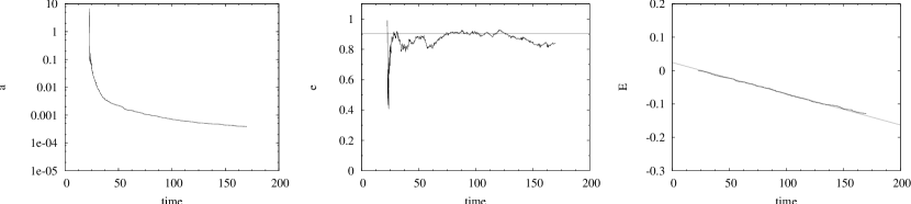
Figure 1.— Example of the typical evolution of the SMBH binaries semi-major axis $a$ (left panel), its eccentricity $e$ (middle panel) and its total energy $E$ (right panel) as a function of time in the classical (Newtonian) gravity models. The lines show the average eccentricity after the binary has formed and the linear fit to the energy loss due to super-elastic scattering. All quantities are given in model units.

Figure 2.— Average rate of energy loss due to purely Newtonian, stellar-dynamical effects as a function of the binaries eccentricity. The symbols represent models with $25$k (open circles) and $50$k (filled circles) field particles, respectively. The horizontal lines indicate the mean values of $|dE/dt|$ for our set of $25k$ (full line) and $50k$ (dashed line) models. The mean value of the combined set is plotted with a dotted line. Note that in our models the energy loss, or equivalently the binaries hardening rate, is basically independent of the eccentricity and – in contrast to spherically symmetric nuclei models – also essentially $N$-independent within the indicated error-bars.

In this section we describe the results of our purely Newtonian simulations, i.e., classical models without any $\cal{P\!N\!}$ corrections. For these fiducial models, the evolution of the binary BHs and the field particles is very similar to the corresponding models reported by Berczik et al. (2006). Due to the relatively high degree of rotation in the models used in this work, the initially axisymmetric nucleus models become dynamically unstable and rapidly develop a rotating triaxial (bar-like) structure. As a result of this global instability and due to the dynamical friction against the stellar background, the two BHs are quickly funneled towards the density center of the nucleus, where they form a binary system in our models typically after some $\Delta t\approx 20$, or some $30$ Myr.

It actually turns out that certain binaries characteristics, such as the time when the binary forms ($t_{\mathrm{form}}$), as well as its orbital elements, are very sensitive to the initial conditions of the stellar distribution. Since the eccentricity of the binary is a crucial quantity for its subsequent evolution towards relativistic inspiral and coalescence, it is important to obtain a statistical sample. Therefore we decided to use nine different realizations of the same galaxy nucleus model, by sampling the underlying distribution function with different initial random seeds. This way, e.g., we find eccentricities of the binaries typically in the range between $0.4$ up to $0.99$. The binaries in our simulations tend to form with the higher eccentricities around $0.9$. However, it cannot be decided at this point whether stochastic encounters between the BHs and the stars, or the global (non-linear) bar-instability plays the dominant role in determining the final binary properties.

Figure 3.— Characteristic timescales as a function of the semi-major axis $a_{\mathrm{h}}$ for a) the Newtonian hardening (thick full line) and b) Peters & Mathews (dotted lines) for orbits with eccentricities $e$ ranging from $0.5$ to $0.9$ (from top to bottom) in steps of $\Delta e=0.1$. The speed of light has been chosen as $c\approx 500$ in model units.

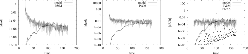
Figure 4.— Time-derivatives of the orbital elements $a$, $e$ and $E$ (from left to right). The gray curves show the discrete differences as calculated from the model directly, and the black curves show the derivatives based on the Peters & Mathews formalism. The dotted curve in the right panel shows the results from the post-Newtonian expression (see Eq. 2-15 in the text).

In Fig. 1 we show an example for the typical time evolution of the (Keplerian) orbital elements for one of the SMBH binaries in our $50$k Newtonian models. In the panels, from left to right, we show the evolution of the semi-major axis $a$, the eccentricity $e$, and the energy $E$ of the binary, respectively. Note that the extremely large values of $a$ and $e$ at early times are due to the fact the the two SMBH are still unbound. Only when they have formed a gravitationally bound pair, i.e., when the binaries energy $E$ becomes negative, the eccentricity $e$ remains below a value of $1$. As one can see in the middle panel, the eccentricity varies only mildly in the subsequent evolution, i.e., when the binary is hard and interacts with the surrounding field particles mainly by super-elastic three-body scattering. Therefore, we calculate some mean eccentricity $\bar{e}$ for each model as indicated by the horizontal line in the middle panel of Fig. 1. We find $\bar{e}$ to be a useful quantity to characterize the binary, but it is important to bear in mind that it provides only a first order approximation, since the real eccentricity may in fact vary with time due to stochastic encounters with field particles.

We find that the loss of energy (Fig. 1, right panel) due to super-elastic three-body encounters is almost constant after roughly $t\gtrsim 30$. The straight line shows the result of a linear least-squares fit to $E(t)$ after the binary has formed. In Fig. 2 we show the resulting slopes $|dE/dt|$ as derived from such linear fitting as a function of $(1-e^{2})$ for our different Newtonian models. The horizontal lines in Fig. 2 indicate the mean values of $dE/dt$ for both the separate and combined sets of our Newtonian $25$k and $50$k models.

Since $E\propto(1/a)$ for a Keplerian orbit, the rate $dE/dt$ provides a direct measure for the hardening rate of the binary $d/dt\,(1/a)$. We find that the hardening rate shows an essentially $N$-independence of both the eccentricity of the binaries’ orbit and the number of field particles used in the models.

The latter result is in good agreement with Berczik et al. (2006) who found only small variations in the hardening rate for models with particle numbers ranging from $25$k to $1$M field particles, which is interpreted as a result of an efficient loss-cone refilling as found in such triaxial, rotating nuclei models.

For our two Newtonian sets of $25$k and $50$k models, we find mean values for $|dE/dt|$ of about $(1.01\pm 0.19)\times 10^{-3}$ and $(0.95\pm 0.17)\times 10^{-3}$, respectively. The hardening rate in our models is found to be essentially $N$-independent within the given error margins. This finding is clearly in accord with the results of Berczik et al. (2006). The mean value of $dE/dt$ for the combined set of models thus results in being roughly $\dot{E}\equiv dE/dt\approx-0.001$.

One can use the results of the previous paragraph to make some simple estimates regarding the binary evolution timescale in the purely Newtonian regime described above. For a Keplerian orbit we get:

$$\frac{da}{dt}=\frac{2\,a^{2}}{G\,m_{1}\,m_{2}}\frac{dE}{dt}\,.$$ (3-1)

We define the binary hardening time in the usual way as

$$\tau_{\mathrm{hard}} \equiv \left|{\frac{1}{a}}{\frac{da}{dt}}\right|^{-1}=\left|{\frac{1}{E}}{\frac{dE}{dt}}\right|^{-1}$$ (3-2)

$$= {\frac{G\,m_{1}\,m_{2}}{2a}}\left|{\frac{dE}{dt}}\right|^{-1}.$$

Writing the rate of change of the binary energy in $N$-body units as $|dE/dt|=10^{-3}\times K$, where $K\approx 1$, this becomes in physical units

$$\tau_{\mathrm{hard}}=9.80\times 10^{3}K^{-1}{\frac{m_{1}\,m_{2}\,r_{c}^{5/2}}{{G}^{1/2}M_{\mathrm{gal}}^{5/2}a}}$$

$$\approx 4.62\times 10^{4}{\mathrm{yr}}{\frac{m_{1}\,m_{2}}{\left(10^{8}\,{\mathrm{M}}_{\odot}\right)^{2}a}}\left({\frac{r_{c}}{10^{2}{\mathrm{pc}}}}\right)^{5/2}\left({\frac{M_{\mathrm{gal}}}{10^{11}M_{\odot}}}\right)^{-5/2}\left({\frac{a}{1\ {\mathrm{pc}}}}\right)^{-1}$$ (3-3)

This expression shows clearly that a constant rate of energy loss corresponds to a gradually increasing timescale for binary hardening. If we assume that the expression holds for arbitrarily small $a$, we can predict a time to coalescence of

$$t_{\mathrm{coal}}-t_{0}=\tau_{\mathrm{hard}}(a_{0})\left({\frac{a_{0}}{a_{\mathrm{coal}}}}-1\right),$$ (3-4)

where $a_{0}=a(t_{0})$ and $a_{\mathrm{coal}}=a(t_{\mathrm{coal}})$ (Ferrarese & Ford, 2005). Setting $a_{0}=1$ pc and $a_{\mathrm{coal}}=(10^{-2}\ldots 10^{-4})\,a_{0}$ gives coalescence times ranging from $\sim 10$ Myr to $1$ Gyr for a galaxy with $M_{\mathrm{gal}}=10^{11}{\mathrm{M}}_{\odot}$ and $r_{\mathrm{c}}=100$ pc. Thus we see clearly that the binaries in our galaxy models would have no difficulty reaching very small separations in a Hubble time, even in the absence of relativistic energy loss.

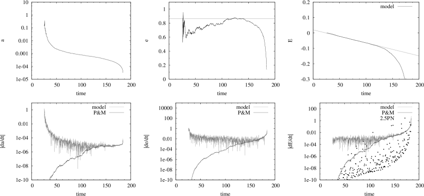
Figure 5.— Time evolution of a SMBH binary orbit in a Newtonian + $2.5\cal{P\!N\!}$ model (using $c=447$). Layout for the upper and lower panels are the same as in Figs. 1 and 4, respectively.

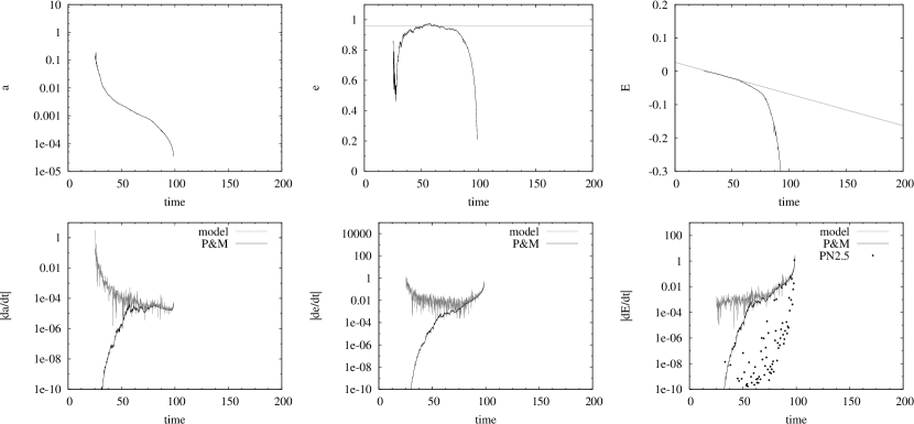
Figure 6.— Example of the time evolution a binary in the Newtonian + full $\cal{P\!N\!}$ models with $c=447$. Same layout as in Fig. 5.

In Fig. 3 we plot both the calculated timescale $\tau_{\mathrm{hard}}$ for the stellar dynamical hardening, as well as the relativistic coalescence timescale $t_{\mathrm{gr}}$ (see Eq. 2-9) for orbits of different eccentricity as a function of their semi-major axis. As one can see, the two involved timescales are of the order of only some hundred time units or Myr, respectively, for the range of eccentricities found in our simulations. These timescales are short enough to allow, on average, for the SMBH binaries to coalesce by the time the next galaxy merger would occur.

In order to test whether the purely Newtonian stellar dynamics in our models is sufficient enough to bring the SMBH binary into the regime where relativistic effects start to become important, we have done the following test: we first calculate the discrete time-derivatives, i.e., finite differences, of the orbital elements and the total energy as directly computed from our simulations. An example is shown in Fig. 4 (gray curves). In a second step we can then use Peters & Matthews’ formalism (Eqs. 2–4) in order to calculate the corresponding orbit-averaged rates, which encode the binary’s secular drift due to the emission of GWs at the lowest, quadrupolar, order. The resulting curves are also plotted in Fig. 4 (black curve). Finally, we use the post-Newtonian expression for the (instantaneous) energy loss due to gravitational wave emission (Eq. 2-15).

One can see that by the time $t\approx 100$ in model units (or some $150$ Myr), the two black holes have reached a separation that is small enough for the relativistic effects to set in and reach the same order of magnitude as the (Newtonian) perturbations from the field particles. This analysis demonstrates that with these rotating King models, the SMBH binary quickly (within a cosmological context) hardens to a point where it reaches the relativistic regime and the final parsec problem can be overcome. In the next section, we study the self-consistent evolution of the (non-spinning) SMBH binaries in the field of stars of the galactic nuclei remnant, including the post-Newtonian corrections up to $2.5\cal{P\!N\!}$ order.

3.2. Models including Post-Newtonian Corrections

To test if the final parsec problem can really be overcome self-consistently just by stellar-dynamical effects and if the binary black holes in our models eventually reach the relativistic inspiral regime, we take the following approach:

We start with models having exactly the same initial conditions for the set of $25$k and $50$k models described in the previous section, but this time we take the $\cal{P\!N\!}$ corrections for the two black hole particles into account. Most numerical simulations of similar kind which are known to us from the literature are restricted – for simplicity – to the first dissipative $\cal{P\!N\!}$ term in the expansion, i.e., the $2.5\cal{P\!N\!}$ correction. The effects of the $1\cal{P\!N\!}$ and $2\cal{P\!N\!}$ , which both are conservative and are known to result in a pericenter shift, have often been neglected. However, these corrections are of lower order in $(v/c)$ as compared to the $2.5\cal{P\!N\!}$ and thus should clearly affect the binary evolution. Therefore, we decided to run all sets of simulations presented below with (a) only including the $2.5\cal{P\!N\!}$ correction and (b) including the full $\cal{P\!N\!}$ corrections up to $2.5\cal{P\!N\!}$. Since higher order corrections such as the $3\cal{P\!N\!}$ term in the equations of motion are of order $c^{-6}$ or smaller, their effect on the dynamical evolution of the BHs are expected to be small as well, and will not affect the main results presented in this work. Hence, we will loosely refer to the models in our set (b) as the ones with full $\cal{P\!N\!}$ corrections. We should note here that the $\cal{P\!N\!}$ corrections in our runs are applied permanently, independent of the BH separation or their relative velocities (see for comparison Aarseth, 2007). Finally, in order to enhance the relativistic effects we use different values of the speed of light $c$ (in models units). We note that by fixing the values for $G$ and $c$, the ratio between the units of mass and length is also fixed. Therefore, one has only one free parameter for setting the corresponding physical units in contrast to classical $N$-body simulations, which are scale-free in that respect.

In Figs. 5 and 6 (upper panels) we show some examples of the evolution of the semi-major axis $a$, the eccentricity $e$ and the total energy $E$ of the binary, respectively.  The corresponding time derivatives, i.e., the discrete, Peters & Mathews and $\cal{P\!N\!}$ as defined in the previous section are shown in the lower panels of these figures, respectively. Both simulations shown in these figures start with identical initial conditions and only differ by the orders of $\cal{P\!N\!}$ corrections taken into account.

At early times, the dynamical evolution of the binary is qualitatively very similar as compared to the evolution in our purely Newtonian simulations (see Figs. 1 and 4): the two BH particles are rapidly driven towards the nuclei center by dynamical friction and the triaxial bar-structure in the stellar nucleus. The black holes form a pair at roughly $t=25$ (or some $37$ Myr, correspondingly). Following the results and interpretation of Berczik et al. (2006), the initially full loss-cone around the black hole binary is quickly depleted and the evolution of the hard binary thereafter takes place in the empty loss-cone regime. Due to the internal rotation and the triaxial structure of the nucleus the loss-cone is re-populated constantly by centrophilic orbits with a rate which is found to be independent of the number of field particles in the model.

During this phase the binary evolution is mainly dominated by just the Newtonian stellar-dynamical effects. The average rate of energy loss during this phase is again of the order of $-0.001$ as has been also found in the Newtonian simulations (Fig. 2). Furthermore, this value is independent of the eccentricity with which the binary has formed and remains constant during the Newtonian dominated phase. That relativistic effects are not yet important during this phase of evolution is supported in the lower panels in Figs. 5 and  6 in which we compare the results from the simulations with the ones as expected by applying Peters & Mathews equations.

The relativistic changes of the orbital elements become of the same order of the Newtonian ones after roughly $t\gtrsim 120$ (in Fig. 5) and $t\gtrsim 60$ (in Fig. 6). More generally, we find that the time of transition from the Newtonian dominated regime to the one in which relativistic effects are of about the same order, depends strongly on the (mean) eccentricity $\bar{e}$ of the binary’s orbit. This result is not surprising since as we have already stated before, the dissipation rate due to gravitational wave emission becomes already important at earlier times for more eccentric binaries.

Finally, at about times $t\gtrsim 140$ and $70$ for Figs. 5 and 6, respectively, the rate of energy loss increases significantly due to the emission of gravitational waves and becomes very non-linear. The loss of orbital energy and angular momentum due to the $2.5\cal{P\!N\!}$ corrections leads to the inspiral and circularization of the orbit, and the binary’s dynamics in this phase is dominated by the relativistic effects, i.e., the binary almost fully completely decouples from the surrounding nucleus.

It is noteworthy that these are the first systematic astrophysical $N$-body simulations which actually follow the evolution of the supermassive black holes from their unbound state, i.e. with order kpc separation, down to the sub-parsec scale close to relativistic coalescence and thus overcome the final parsec problem self-consistently. It seems that the origin of the latter problem partly has been the use of over-simplified models for the galactic nuclei, i.e., assuming spherically symmetric distributions without (net) angular momentum.

4. Discussion

Figure 7.— Comparison of models using $2.5\cal{P\!N\!}$ corrections only (green lines) and using the full $\cal{P\!N\!}$ corrections (red lines). Shown are the inverse of the semi-major axis (thick lines) and the eccentricity (thin lines) as a function of time.

We have presented one of the first extensive sets of stellar-dynamical $N$-body simulations including full post-Newtonian corrections up to $2.5\cal{P\!N\!}$ for the dominant two-body interaction between two supermassive black holes, which covers self-consistently all evolutionary phases from an initially unbound SMBH binary with separations of order $10^{3}$ pc down to the final relativistic coalescence (but see Aarseth 2003a for an early pioneering work). Our initial conditions are still special but plausible: a “young” galactic merger remnant is represented by a flattened, rotating stellar nucleus with the two SMBHs at a separation of initially some $10^{3}$ pc. This is a more general class of initial models than used in most other papers on the subject (Makino et al., 1993; Milosavljević & Merritt, 2001; Hemsendorf, Sigurdsson & Spurzem, 2002; Aarseth, 2003a; Makino & Funato, 2004; Berczik et al., 2005). This could be seen as one possible solution of the long-standing final parsec problem for black hole mergers (Begelman et al., 1980), as in this class of models we find convergence in the hardening rates at low $N$. This is the result of a dynamical regime where the supply of the stars into the loss-cone region is essentially collisionless and presumably guaranteed by a family of centrophilic orbits associated with this non-spherical potential (cf. Sections 1.1 and 5).

In the following we discuss in further depth some dynamical properties of our models and observational consequences of our results for gravitational wave instruments.

4.1. Effect of the different $\cal{P\!N\!}$ orders

We have performed of order $150$ different simulations, varying the initial data (statistical realization, particle numbers) and different physical scalings (speed of light, different $\cal{P\!N\!}$ orders). In all models that include the $\cal{P\!N\!}$ equations of motion for the black holes we are able to follow the binaries’ evolution down to the relativistic inspiral and virtually to coalescence. Based on our simulations we find that inclusion of the $1\cal{P\!N\!}$ and $2\cal{P\!N\!}$ corrections, which have been neglected in most earlier works (again with the notable exception of Aarseth (2003a)), strongly affects the dynamical evolution of the binary. Fig. 7 shows this, where we directly compare the evolution of $1/a$ and eccentricity as a function of time for two otherwise equal models with full $\cal{P\!N\!}$ and $2.5\cal{P\!N\!}$ corrections only, respectively. The time of coalescence differs by almost a factor of two between these two cases. We find that part of the reason for this diverging behavior is the different eccentricity with which the binary forms. Using full $\cal{P\!N\!}$ corrections rather than only $2.5\cal{P\!N\!}$ changes the details of the binary’s trajectory already during their first encounters. Consequently later on, the binary forms with different orbital elements. Since all close encounters in the system – up to the one leading to the binary formation – are stochastic (due to the dynamical instability of close few-body encounters) we do do not find any preferred systematic trend in our models towards higher or lower eccentricities between the two types of simulations as a function of the type of $\cal{P\!N\!}$ corrections used.

4.2. Orbital properties of SMBH binaries

In Fig. 8 we show the distribution of eccentricities $\bar{e}$ obtained from the sample of all our simulations. It clearly shows that the binaries form preferentially with very high eccentricities. This is favored by the transient triaxial feature in our models (see also, Berczik et al., 2006) which brings the two black holes together with relatively small impact parameter. Since galactic mergers lead dominantly to the formation of stellar bars or other triaxial configurations (see, e.g., Naab, Khochfar, & Burkert, 2006; Jesseit et al., 2007; Johansson, Naab & Burkert, 2008), we expect that high eccentricities in SMBH binaries after galactic mergers are a robust phenomenon occurring in many real cases. Furthermore, the merger of spherical models of galactic nuclei along nearly-parabolic trajectories also leads to the formation of SMBH binaries with a similar distribution of high eccentricities (Preto et al.,, submitted).

It is known that during the relativistic inspiral, emission of GWs leads to the circularization of the binary (Peters, 1964). In the same Fig. 8, we therefore also show the (shaded) histogram for the binary’s eccentricities when their semi-major axis has fallen down to $100$ Schwarzschild radii $R_{\mathrm{BH}}$, for the runs with the realistic values of $c=447$. We can clearly see that, although circularization has substantially reduced the binaries’ eccentricity, the remaining distribution at such small separation is still significantly different from zero. Since the orbital eccentricity of the binaries is very important to predict gravitational waveforms from these binaries, and the expected distribution of their orbital parameters strongly determines the complexity of the data analysis for gravitational wave instruments such as the planned LISA satellites (e.g., Babak et al., 2008), we are currently generalizing the present study to a wider range of more realistic initial conditions.It may be interesting to note that this type of statistics provides an astrophysically motivated set of initial conditions for numerical relativity simulations of SMBH binary mergers. During the last couple of years several groups have made significant progress in modeling black hole mergers by the solution of the full Einstein equations and of numerical-relativity simulations (cf. Rezzolla et al. (2008) and citations $8$–$13$ therein).

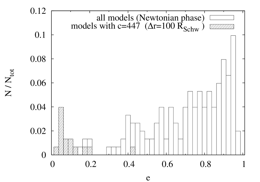
Figure 8.— Distribution of eccentricities of the binaries in the Newtonian regime. The white histogram shows the normalized distribution of eccentricities of SMBHs in the Newtonian evolutionary phase. The gray histograms shows the distribution of eccentricities at later times, i.e., when the binary have reached a separation of $100$ Schwarzschild radii. Note that at these short separations the majority of the orbits still has not yet fully circularized.

Figure 9.— Example of the time a binary spends at different semi-major axis intervals. The solid line shows a Gaussian fit to the histogram used to determine expectation value of $a$ and $\sigma$.

Figure 10.— Expectation value of $\langle a\rangle$ as a function of the orbital eccentricity for simulations with $c=447$. The fitted line only takes the – more realistic – full $\cal{P\!N\!}$ models into account.

Figure 11.— Probability to find the SMBH binaries with separations below some given maximum semi-major axis. The different lines correspond to orbits with different eccentricity as given in the legend.

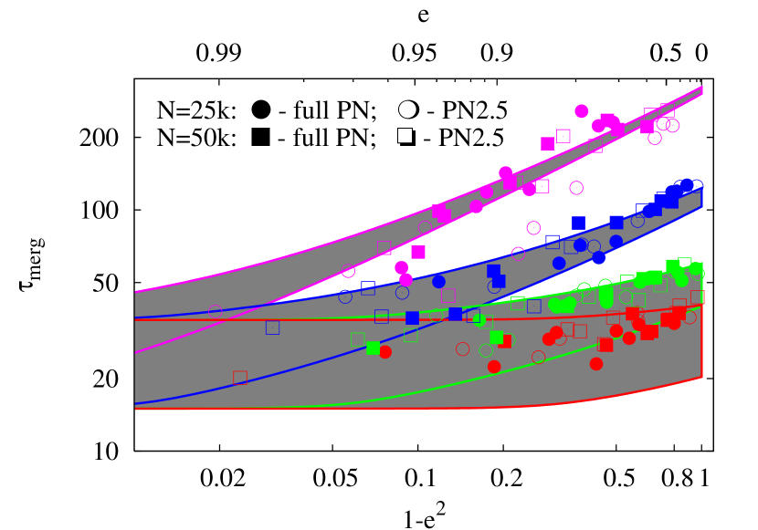
Figure 12.— Merging time $T_{\mathrm{merge}}$ of the SMBH binaries for models with different values of $c$ ($c=14$:black; $c=44$:red; $c=141$:green; $c=447$: blue. The shaded region indicate the predicted merging times using Eq. 4-1 as given in the text. The upper and lower boundaries of the shaded regions account for different formation times $T_{\mathrm{form}}$ of the binary. Since the Newtonian dominated regime lasts longer for models with $c=447$, the eccentricity of the orbit varies stronger and results in a larger scatter in the plot. The are no clear differences between models with $2.5\cal{P\!N\!}$ only and full $\cal{P\!N\!}$ corrections.

As we have described in Sec. 3.2 we can distinguish three dynamical phases of SMBH binary evolution: (1) Newtonian phase, (2) mixed phase and (3) relativistic phase. It is thus interesting to see how much time a binary will spend the corresponding separations. In Fig. 9 we plot a histogram showing the time the binary spends at a given semi-major axis normalized to the total binary lifetime, measured from its formation till coalescence. The binary orbit of the model selected for Fig. 9 spends some ten per cent during its evolution at semi-major axis of $10^{-3}$, or $1$ pc in physical units. We fit a Gaussian distribution to the binned data to provide a rough measure of the average value $\langle a\rangle$ and of the dispersion around it.

In Fig. 10 we then plot $\langle a\rangle$ as a function of the orbital eccentricity. While the SMBH binaries with high eccentricity tend to have larger $\langle a\rangle$, the fitted slope of the double logarithmic plot of $\langle a\rangle$ vs. $(1-e)$ is $-0.87$. We conclude therefore that the average pericenter $r_{\mathrm{p}}=\langle a\rangle(1-e)$ of the SMBH orbit at any given average $\langle a\rangle$ has a remarkably small variation, i.e., is nearly constant. Therefore – to first order – the orbits of SMBH binary in our models form a one-parameter family. This result is relevant and interesting for the determination of gravitational wave backgrounds in the ultra-low and low-frequency areas from SMBH binaries in the universe: Eccentric SMBH binaries emit gravitational waves with a spectrum of frequencies $g(n,e)$, where $n$ denotes the higher harmonics over the basic mode of the circular orbit (see Appendix). The harmonic which leads to the maximal emission of gravitational waves $n_{\mathrm{max}}(e)$ is for high eccentricities ($e\geq 0.8$) completely determined by the frequency of motion at pericenter $n_{\mathrm{peri}}\propto(1-e)^{-3/2}$ (Pierro et al., 2001; Amaro-Seoane et al., 2008). Thus for every value of average semi-major axis $\langle a\rangle$ there exists a typical pericenter value and thus a typical gravitational wave spectrum. The expected signals of these objects (in particular highly eccentric ones) lie in the pulsar timing and lower LISA bands (see for more details, including triple black holes, also Enoki & Nagashima, 2007; Hoffman & Loeb, 2007).

Fig. 11 illustrates the cumulative probability to find the SMBH binary with a semi-major axis smaller than $a$. For each of our runs with full $\cal{P\!N\!}$ terms and realistic value of $c=447$ one curve is plotted in the figure. From this information one can deduce that SMBH binaries with high eccentricity stay longer at larger $a$, which is an information consistent with the previous figure. The probabilities are normalized for each run separately, therefore these data cannot be used to determine probability distributions of $a$ for samples of SMBH binaries in the universe.

4.3. Timescales for SMBH coalescence

In Sec. 3.1 we estimated the time required for the coalescence of SMBH binaries in our models driven by stellar-dynamical effects only. On the other hand, using the pure relativistic estimate of the coalescence timescale $t_{\mathrm{gr}}$ (Eq. 2-9), we find for typical semi-major axis values of $a_{\mathrm{h}}\approx 10^{-2}\ldots 10^{-4}$ and eccentricities of $e\approx 0.5\ldots 0.99$ that the resulting timescale covers a range of $t_{\mathrm{gr}}\approx 10^{9}\ldots 10^{-4}$ in our model units. The interpretation of these numbers is that for small semi-major axes $a$ and high eccentricities the two SMBHs basically directly plunge, while for larger $a$ and moderate $e$ the relativistic timescale becomes unreasonable large. The evolution and hardening of the binary in such case would therefore mainly be driven by the Newtonian stellar-dynamics over some time period. Eventually, the semi-major axis may reach small enough values for the emission of gravitational waves to become efficient. The binary hardening would then equally be driven by both the classical Newtonian and the relativistic effects, before the latter eventually takes over, i.e., when the binary dynamically decouples from the stellar background.

To get a more precise estimate of the time until relativistic coalescence, we numerically integrate the following differential equation:

$$T_{\mathrm{merg}}=T_{\mathrm{form}}+\int\left[\left(\frac{\partial a}{\partial t}\right)_{\mathrm{hard}}+\left(\frac{\partial a}{\partial t}\right)_{\mathrm{P\&M}}\right]dt\,,$$ (4-1)

where the corresponding $da/dt$ are given by Eq. 2-5 and 3-1, respectively. For the integration we start with semi-major axis separation of some $10^{-3}$ and different eccentricities. For the formation time of the binary we assume $T_{\mathrm{form}}=15$ and $35$ as a lower and upper limit, respectively.

In Fig. 12 we plot the coalescence time as measured from our simulations for different values of $c$ as a function of eccentricity. The results are then compared to the results obtained from integration of the above Eq. 4-1. Considering the different times it takes the binaries to form a bound pair in the simulations our results agree (within the error limits) with the theoretical value.

Not surprisingly, we find that the merging time increases with increasing values of $c$, since the relativistic corrections decrease for simulations starting with the same configuration. However, since the hardening rate due to super-elastic scattering with the binary is found to be constant in our simulations, we expect an upper limit of $T_{\mathrm{merg}}$ of roughly $500$ time units. It is important to note that in all our simulations the two black hole coalesce in less then $0.5$ Gyr after they have formed a bound pair! Therefore we conclude that our results provide a dynamical substantiation to the picture of prompt SMBH coalescence advocated by Volonteri et al. (2003) and Sesana et al. (2005, 2007). Moreover, we should also note that these times for black hole coalescences are of the same order as the average interval between consecutive mergers (cf. e.g. Fig. $2$ in Khochfar & Burkert (2001), and Khochfar & Burkert (2006)). Such timescales make it unlikely that there is enough time for a third black hole to interact with the binary before it has coalesced. If three-body interactions between SMBHs were the norm, then it would be quite difficult to understand the notably small amount of scatter in the $M-\sigma$ relation, as well as the scarcity of observational evidence for off-centered nuclei. Note, however, that some fraction of triple interactions of SMBHs may be present in the universe and could cause extremely large eccentricities (e.g. through Kozai oscillations) and become visible through pulsar timing or even in the lower LISA band at comparatively large separations (orbital time scales) (Iwasawa, Funato & Makino, 2006; Hoffman & Loeb, 2007; Amaro-Seoane et al., 2008; Iwasawa, Funato & Makino, 2008).

4.4. Gravitational Wave Signal

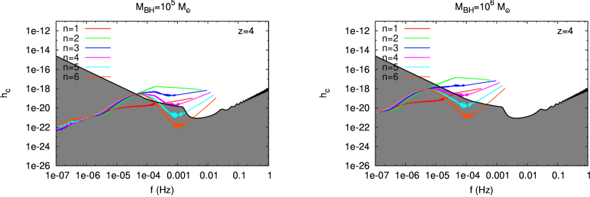
Figure 13.— Locus of a SMBH binary from one of our simulations, for the first six harmonics, in the LISA sensitivity diagram during their final inspiral and coalescence. The black curve is the LISA sensitivity obtained from the online generator (see text). The dimensionless characteristic strain $h_{c}$ is plotted against the observed frequency. This case corresponds to a calculation including all $\cal{P\!N\!}$ corrections term up to the radiation reaction at $2.5\cal{P\!N\!}$ level. The orbital parameters adopted in this case were the full $2\cal{P\!N\!}$ accurate tangential eccentricity $e_{\mathrm{t}}$ and semi-major axis $a$ (Memmesheimer et al., 2004). Left panel: the binary MBH has total mass $m_{12}=2\times 10^{5}M_{\odot}$; right panel: $m_{12}=2\times 10^{6}M_{\odot}$; placed at redshift $z=4$.

Merger events of SMBH binaries are expected to be one of the brightest possible sources of gravitational wave emission to be detected by LISA (Danzmann, 1997; Phinney, 2005): The Laser Interferometer Space Antenna, a proposed space-borne gravitational wave observatory, scheduled for launch in 2018+, is most sensitive to gravitational waves in the low-frequency regime ($10^{-4}$ – $0.1$ Hz); for SMBHs of more than about $10^{7}{\mathrm{M}}_{\odot}$ LISA will preferentially detect the final merger and ringdown phases (Babak et al., 2008), while for smaller masses earlier evolutionary phases of SMBH evolution will become detectable in the LISA band, in particular for eccentric SMBHs (see discussion and references in Sect. 4.3).

In most of the present literature the strain amplitude of the gravitational wave is usually estimated under the assumption of circular orbits. This has been motivated by the idea that massive binary systems are expected to have been completely circularized due to the emission of gravitational waves (see, e.g., Peters, 1964; Sesana et al., 2005) by the time they enter the LISA frequency band. In this section we will use our results to test this assumption. The details on how to extract the information on the gravitational wave strain amplitude from our numerical simulations calculation are given in the Appendix.

The space-based gravitational wave detector LISA will be sensitive to signals of inspiralling compact objects with up to the maximum total mass $M_{12}\approx 7.5\times 10^{6}$ M_⊙, where $M_{12}$ is the total mass of the binary. Due to the involved low frequencies of the signal, such sources are out of reach of current ground-based detectors. The physical units adopted in Sec. 2.1 translate into black hole masses of about $10^{9}$ M_⊙ in our simulations. Black hole binaries in this mass regime, however, will inspiral with frequencies even lower than those of the LISA band and thus would not be detectable by LISA before their actual coalescence.

In order to follow the black hole binary inspiral up to frequencies in range of interest for LISA, i.e, $f\geq 10^{-4}$ Hz, we first need to rescale our models to binary masses of order of $10^{5}$ or $10^{6}$ M_⊙. As mentioned earlier, the speed of light in model units scales as $c\propto(R/M)^{1/2}$, where $R$ and $M$ are the units for length-scale and mass, respectively. Since $c$ is already given with a fixed value from our simulations, by changing our unit of mass by factors $10^{-3}-10^{-4}$, the length-scale automatically changes to $0.1$ or $1$ pc, respectively. Finally, following the results of Sesana et al. (2007), we place the system at the redshift $z=4$, where LISA’s detection rate for objects of that mass range is expected to be significant.

Before actually calculating the strain amplitude of the gravitational wave signal, we increase the time-resolution of our output data for the black hole’s trajectory during the late phases of inspiral. This is done by evolving the binary in isolation, starting with initial conditions (in the binaries center of mass frame) as given from the large-scale simulations at a stage when it is already decoupled from the surrounding stellar system, i.e., when the binary evolution is dominated by relativistic dynamics (compare Fig. 6). We convince ourselves that the binary is really decoupled from the stellar system by comparing the evolution of its orbital elements to the one of the ”low” time-resolution. In fact, during the late stages of inspiral the perturbations from stars vary over timescales much longer than both the orbital period and the time for coalescence (at that moment) which allows us to safely ignore them.

Using the information of the combined time-series of the binary evolution we then calculate the orbital elements in the $\cal{P\!N\!}$ generalization (Memmesheimer et al., 2004). These allow us to calculate the different modes of the characteristic strain amplitude $h_{c,n}$ using Eq. A from the Appendix.

In Fig. 13 we show $h_{c,n}$ for the first six harmonics of the signal generated by the inspiral in one of our $50$k models for (rescaled) binary masses of $2\times 10^{5}$ M_☉ (left panel) and $2\times 10^{6}$ M_☉ (right panel). The LISA sensitivity curve $S_{h}(f)$ displayed in the figures was generated by the Online Sensitivity Curve Generator with default settings, corresponding to a three year observation period (Larson, 2007). We confirm that the BH binaries in the mass range $10^{5}-10^{6}$ M_☉ indeed enter the LISA frequency band during the relativistic inspiral in our simulations. The height of $h_{c,n}$ above the sensitivity curve in Fig. 13 provides an approximate indication of the signal-to-noise ratio (SNR; see also Appendix) and is found to be high enough for detection by LISA.

As a consequence of the very high initial eccentricity with which the MBH binaries form in our simulations (compare Fig. 8), they reach the LISA band with an eccentricity which may be significantly different from zero – the exact distribution depending on the redshift $z$ of the sources (Preto et al., in prep.). As a result, there will be a significant contribution to the measured power from higher harmonics $f_{n}=n\,f_{\mathrm{orb}}/(1+z)$, with $n\geq 2$ (note that $n=2$ for a circular orbit). This can be seen from the plots shown here, where several harmonics contribute significantly to the GW signal and are well above the threshold for detection. Furthermore, we find that, as the binary chirps in the LISA band, it circularizes quite rapidly with the consequence that the $n=2$ harmonic always becomes dominant at the last stages of the inspiral.

These findings may have an important impact on the accurate computation of the inspiral waveforms as well as potentially leading to an increased upper limit of the range of detectable masses by LISA. Based on our results we suggest that orbits with non-vanishing eccentricities should indeed seriously be considered for the LISA data analysis. Further details and discussion of the consequences for the LISA detection of SMBH binary inspirals are beyond the scope of this work and will be published elsewhere (Preto et al., in prep.).

5. Conclusions

We present the first $N$-body models which self-consistently follow the evolution of binary supermassive black holes in merged galaxies from kiloparsec separations down to gravitational-wave-induced coalescence, and in which the early evolution of the binary is driven by collisionless loss-cone repopulation, allowing the results to robustly be scaled to real galaxies. Our simulations include post-Newtonian corrections to the equations of motion of the SMBH binary up to order $2.5\cal{P\!N\!}$; we show that inclusion of the energy-conserving $1\cal{P\!N\!}$ and $2\cal{P\!N\!}$ terms is also crucial for obtaining the correct time dependence of the binary orbital parameters. We identify evolutionary phases in which the binary is still evolving due to stellar encounters but in which relativistic corrections to its two-body motion are also important, thereby showing that the consideration of all $\cal{P\!N\!}$ orders in the $N$-body simulations is necessary for an accurate prediction of its orbital elements evolution. The SMBH binaries in our simulations often form with large eccentricities, and these high eccentricities are maintained during the Newtonian phases of the evolution. We show that the gravitational wave signal measured by an interferometer like LISA would contain significant contributions from high-order harmonics from GWs emitted from binaries at cosmological distances, and that the nature of the signal can depend strongly on the dynamical history of the binary prior to its entering the gravitational wave dominated regime.

We have shown that supermassive black hole binaries in galactic nuclei can overcome the stalling barrier and will reach the relativistic coalescence phase in a timescale shorter than the age of the universe. A gravitational wave signal expected for the LISA satellite from these SMBH binaries is expected, in particular due to the high eccentricity of the SMBH binary when entering the relativistic coalescence phase. We present for the first time a comprehensive set of models which cover self-consistently the transition from the Newtonian dynamics, dynamical friction phase (with yet unbound SMBH binary) to the situation when relativistic, post-Newtonian corrections start to influence the relative SMBH motion. After the shrinking time scale becomes very short the binary decouples from the rest of the galactic nucleus and can be treated as a relativistic two-body problem. We follow this evolution formally to the coalescence of the two black holes using $\cal{P\!N\!}$ terms of up to order $2.5\cal{P\!N\!}$ and determine the gravitational wave emission in different modes relative to the LISA sensitivity curve. We find that the orbital parameters of a SMBH binary, when entering the LISA band, depends on the previous dynamical history - in particular there exists a phase where the SMBH binary is still partially coupled to the stellar environment via three-body encounters, but relativistic corrections to its two-body motion already play a role.

Since purely Newtonian models of SMBH binaries in rotating galactic nuclei (Berczik et al., 2006) have shown a quasi-$N$-independence of the stellar-dynamical driven hardening rates, we conclude that the results obtained in this paper regarding the time required until relativistic merger holds for galactic nuclei with realistic parameters. In this work we limited ourselves to models with particle numbers up to $50$k only, however, due to the independence of the results in the Newtonian phase from $N$ in the current work and in Berczik et al. (2006), we do not expect any significant changes in our main results for models with $N>50$k.

It should be noted, however, that our results show a strong dependence on initial conditions, and that our initial model is a very simple approximation to a post-merger galactic nucleus. Therefore our conclusion from this work can only be that it is possible to reach relativistic coalescence in a reasonable time ($10^{8}$ years). Any prediction of event rates for LISA would, however, require a more careful estimate of the distribution of parameters for a realistic set of mergers, e.g. by taking data from semi-analytic merger trees, similar to Sesana et al. (2005). This is the subject of presently ongoing work.

We have also examined the effect of using $2.5\cal{P\!N\!}$ alone or full $\cal{P\!N\!}$ corrections. Simple two-body $\cal{P\!N\!}$ experiments show significant differences of the BHs trajectories, and we find generally a dependence of the merging time in the two cases. Different orbital parameters of the SMBH binary in the final phase would have a major impact on the waveforms of the GWs. However, the computation of the latter also requires simulations with higher $\cal{P\!N\!}$ corrections, at least up to order ${\cal O}({c}^{-6})$, i.e., $3\cal{P\!N\!}$ in the equations of motion. This is beyond the scope of the current paper.

Results on whether our simulated SMBH binary will fall into the LISA frequency band and at which frequencies will be discussed in a cosmological context in a forthcoming paper.

Appendix A Appendix material

Any gravitational wave carries energy: The total energy carried by a wave is $E\sim N(f)\ h^{2}$, where $N(f)$ is the number of cycles the wave spends on a frequency interval $\Delta f\sim f$ around the frequency $f$. It is customary to define a characteristic strain $h_{\mathrm{c}}$ corresponding to an observation with duration $\tau\gtrsim N(f)/f$ by $h_{\mathrm{c}}(f)=\sqrt{N(f)}\ h(f)$. In this case, the signal is not monochromatic and we observe its chirp as it shifts to higher frequency during the observation. However, in case the observation time $\tau\lesssim N(f)/f$, the signal is approximately monochromatic and its amplitude is essentially limited by the observing time rather than by the intrinsic properties of the system and, as a result, $h_{\mathrm{c}}=\sqrt{\tau f}\ h(f)$ (Thorne, 1987).

In the relativistic inspiral phase, the back-reaction from the GW emission (energy balance argument) dominates the binary’s orbital decay (Blanchet, 2006). The number of cycles around a given frequency $f$ can be estimated to be

$$N(f)\sim{\dot{f}_{\mathrm{r}}}/{f_{\mathrm{r}}^{2}}=\frac{5{c}^{5}}{96\pi^{8/3}}{G}^{-5/3}\mathcal{M}^{-5/3}f_{\mathrm{r}}^{-5/3},$$ (A1)

where the orbit is described in terms of the (instantaneous) Kepler elements, the binary’s chirp mass is $\mathcal{M}=m_{1}^{3/5}m_{2}^{3/5}/(m_{1}+m_{2})^{1/5}$, and $f_{\mathrm{r}}$ is the orbital frequency in the source’s rest frame. Following Peters & Mathews (1963), the orbital frequency shifts at a rate given by

$$\dot{f}_{\mathrm{r}}=\frac{df_{\mathrm{r}}}{da}\frac{da}{dt}=\frac{96\pi^{8/3}}{5c^{5}}G^{5/3}\mathcal{M}^{5/3}f_{r}^{11/3}.$$ (A2)

The solution $f_{\mathrm{r}}$ to Eq. A2 blows up in a finite time $\tau_{\mathrm{coal}}$, which is used to denote the coalescence time. For a given frequency $f_{\mathrm{r}}$ the time till coalescence can by calculated according to the following expression:

$$\tau_{{\mathrm{coal}}}\approx\frac{N(f_{\mathrm{r}})}{f_{\mathrm{r}}}\approx\frac{5{c}^{5}}{96\pi^{8/3}}{G}^{-5/3}\mathcal{M}^{-5/3}f_{\mathrm{r}}^{-8/3}.$$ (A3)

Assuming a Keplerian orbital parametrization, the strain amplitude for the $n^{\mathrm{th}}$ harmonic (after sky averaging) is given by

$$h_{n}(f)=\sqrt{h_{+}^{2}+h_{\times}^{2}}=\frac{37\pi^{2/3}}{16}\frac{G^{5/3}\mathcal{M}^{5/3}}{r(z){c}^{4}}f_{\mathrm{r}}^{2/3}\sqrt{g(n,e)}.$$ (A4)

Note that $r(z)$ is the comoving distance (as a function of cosmological redshift $z$) to the source and $g(n,e)$ represents the normalized relative power spectrum in the $n^{\mathrm{th}}$ harmonic of the GW signal (Peters & Mathews, 1963):

$$g(n,e)=\frac{n^{4}}{34}\left\{\left[J_{n-2}(ne)-2eJ_{n-1}(ne)+\frac{2}{n}J_{n}(ne)+2eJ_{n+1}(ne)-J_{n+2}(ne)\right]^{2}\right.$$

$$\left.+(1-e^{2})\left[J_{n-2}(ne)-2J_{n}(ne)+J_{n+2}(ne)\right]^{2}+\frac{4}{3n^{2}}J_{n}^{2}(ne)\right\},$$ (A5)

where the $J_{n}$ are Bessel functions of the first kind. The characteristic strain $h_{c,n}$ can therefore be written as

$$h_{c,n}(f) = \sqrt{N}\ h\sim\frac{37}{64\pi^{2/3}}\sqrt{5/6}\frac{{G}^{5/6}\mathcal{M}^{5/6}}{c^{3/2}R(z)}\ \sqrt{g(n,e)}\ f_{\mathrm{obs}}^{-1/6},\hskip 18.00005ptN\lesssim f_{\mathrm{obs}}\,\tau$$

$$h_{c,n}(f) = \sqrt{f\tau}\ h\sim\frac{37\pi^{2/3}}{16}\frac{G^{5/3}\mathcal{M}^{5/3}}{c^{4}R(z)}\sqrt{g(n,e)}\ \sqrt{\tau}\ f_{\mathrm{obs}}^{7/6},\hskip 30.00005ptN\gtrsim f_{\mathrm{obs}}\,\tau.$$

Note that the frequency seen in the detector is given by $f_{\mathrm{obs}}=f_{\mathrm{r}}/(1+z)$, where $f_{\mathrm{obs}}$ is the frequency measured in the binary’s reference frame. The knee frequency separates the two regimes

$$f_{\mathrm{knee}}=N(f)f_{\mathrm{obs}}\approx\frac{1}{\pi}\left(\frac{5}{96\tau}\right)^{3/8}\frac{{c}^{15/8}}{{G}^{5/8}\mathcal{M}^{5/8}}\,\left(1+z\right)^{-1}.$$ (A7)

Note that the knee frequency decreases if the observation time $\tau$ increases.

The GW signal is said to come into band when $h_{c,n}(f)\geq\langle f\ S_{h}(f)\rangle^{1/2}$, where $S_{h}(f)$ is the instrumental strain noise spectrum (in Hz^-1) and the brackets denote sky-averaging. The LISA sensitivity curve $S_{\mathrm{h}}(f)$ displayed in the figures was generated by the Online Sensitivity Curve Generator with default settings, corresponding to a three year observation period (Larson, 2007). The height of $h_{c}$ above the sensitivity curve provides an approximate indication of the signal-to-noise ratio (SNR); however, the integrated SNR should be computed as

$$\left(\mathrm{SNR}\right)^{2}=\int_{f_{{\mathrm{min}}}}^{f_{{\mathrm{max}}}}\frac{df}{f}\ \frac{h_{c}^{2}(f)}{\langle f\ S_{h}(f)\rangle}.$$ (A8)

References

- Aarseth (1985) Aarseth, S.J. 1985, in Direct Methods for -body Simulations, ed. J.U. Brackbill, & B.I. Cohen (Academic Press), p. 337
- Aarseth (1999) Aarseth, S.J. 1999, PASP, 111, 1333
- Aarseth (2003a) Aarseth, S.J. 2003a, Ap&SS, 285, 367
- Aarseth (2003b) Aarseth, S.J. 2003b, Gravitational -body Simulations (Cambridge, UK: Cambridge University Press)
- Aarseth (2007) Aarseth, S.J. 2007, MNRAS, 378, 285
- Amaro-Seoane et al. (2008) Amaro-Seoane, P., Benacquista, M., Hoffman, L., Eichhorn, C., Spurzem, R., & Makino, J., submitted to MNRAS
- Andrade, Blanchet & Faye (2001) Andrade, V.C., Blanchet, L., & Faye, G. 2001, Class. Quantum Grav., 18, 753
- Babak et al. (2008) Babak, S., Hannam, M., Husa, S., & Schutz, B. 2008, arXiv:0806.1591
- Begelman et al. (1980) Begelman M.C., Blandford R.D., & Rees M.J. 1980, Nature, 287, 307
- Berentzen et al. (2008) Berentzen, I., Preto, M., Merritt, D., Berczik, P., & Spurzem, R. 2008, Astron. Nachr., 329, 904
- Berczik et al. (2005) Berczik, P., Merritt, D., & Spurzem, R. 2005, ApJ, 633, 680
- Berczik et al. (2006) Berczik, P., Merritt, D., Spurzem, R., & Bischoff, H.-P. 2006, ApJ, 642, L21
- Berentzen et al. (2008) Berentzen, I., Preto, M., Berczik, P., & Spurzem, R. 2008, Astron. Nachr., 329, 904
- Bianchi et al. (2008) Bianchi, S., Chiaberge, M., Piconcelli, E., Guainazzi, M., & Matt, G. 2008, MNRAS, 386, 105
- Blanchet (2006) Blanchet, L., 2006, in Living Rev. Relativity 9, 4. URL (cited on June 2007): http://www.livingreviews.org/lrr-2006-4
- Danzmann (1997) Danzmann, K. 1997, Class. Quantum Grav., 14, 1399
- Dotti et al. (2007) Dotti, M., Colpi, M., Haardt, F., & Mayer, L. 2007, MNRAS, 379, 956
- Enoki & Nagashima (2007) Enoki, M., & Nagashima, M. 2007, Progress of Theoretical Physics, 117, 241
- Ernst et al. (2007) Ernst, A., Glaschke, P., Fiestas, J., Just, A., & Spurzem, R. 2007, MNRAS, 377, 465
- Escala et al. (2004) Escala, A., Larson, R. B., Coppi, P. S., & Mardones, D. 2004, ApJ, 607, 765
- Escala et al. (2005) Escala, A., Larson, R. B., Coppi, P. S., & Mardones, D. 2005, ApJ, 630, 152
- Ferrarese & Ford (2005) Ferrarese, L., & Ford, H. 2005, Space Sci. Rev., 116, 523
- Fukushige et al. (2005) Fukushige, T., Makino, J., & Kawai, A. 2005, PASJ, 57, 1009
- Gerhard & Binney (1985) Gerhard O.E. & Binney J. 1985, MNRAS, 216, 467
- Harfst et al. (2007) Harfst, S., Gualandris, A., Merritt, D., Spurzem, R., Portegies Zwart, S., & Berczik, P. 2007, New A, 12, 357
- Hemsendorf, Sigurdsson & Spurzem (2002) Hemsendorf M., Sigurdsson S., & Spurzem R. 2002, ApJ, 581, 1256
- Hoffman & Loeb (2007) Hoffman, L., & Loeb, A. 2007, MNRAS, 377, 957
- Iwasawa, Funato & Makino (2006) Iwasawa, M., Funato, Y., & Makino, J. 2006, ApJ, 651, 1059
- Iwasawa, Funato & Makino (2008) Iwasawa, M., Funato, Y., & Makino, J. 2008, arXiv:0801.0859
- Jesseit et al. (2007) Jesseit, R., Naab, T., Peletier, R. F., & Burkert, A. 2007, MNRAS, 376, 997
- Johansson, Naab & Burkert (2008) Johansson, P. H., Naab, T., & Burkert, A., arXiv:0802.0210
- Kazantzidis et al. (2005) Kazantzidis, S., et al. 2005, ApJ, 623, L67
- Khochfar & Burkert (2001) Khochfar, S., & Burkert, A. 2001, ApJ, 561, 517
- Khochfar & Burkert (2006) Khochfar, S., & Burkert, A. 2006, A&A, 445, 403
- King (1966) King, I.R. 1966, AJ, 71, 276
- Komossa et al. (2003) Komossa S., Burwitz V., Hasinger G., Predehl P., Kaastra J.S., & Ikebe, Y. 2003, ApJ, 582, L15
- Kupi et al. (2006) Kupi, G., Amaro-Seoane, P., & Spurzem, R. 2006, MNRAS, 371, L45
-
Larson (2007)
Larson, S.L., 2007, in A modern astrophysical laboratory, in LISC, the LISA International
Science Community
http://www.lisa-science.org/resources/introductory-lisa-material, 2007. - Libeskind et al. (2006) Libeskind, N. I., Cole, S., Frenk, C. S., & Helly, J. C. 2006, MNRAS, 368, 1381
- Löckmann & Baumgardt (2008) Löckmann, U., & Baumgardt, H. 2008, MNRAS, 384, L323
- Longaretti & Lagoute (1996) Longaretti, P.-Y., & Lagoute, C. 1996, A&A, 308, 453
- Madau et al. (2004) Madau, P., Rees, M. J., Volonteri, M., Haardt, F., & Oh, S. P. 2004, ApJ, 604, 484
- Makino (1997) Makino, J. 1997, ApJ, 478, 58
- Makino & Aarseth (1992) Makino, J., & Aarseth, S.J. 1992, PASJ, 44, 141
- Makino et al. (1993) Makino J., Fukushige T., Okumura S.K., & Ebisuzaki T. 1993, PASJ, 45, 303
- Makino & Funato (2004) Makino, J., & Funato, Y. 2004, ApJ, 602, 93
- Mayer et al. (2007) Mayer, L., Kazantzidis, S., Madau, P., Colpi, M., Quinn, T., & Wadsley, J. 2007, Science, 316, 1874
- Memmesheimer et al. (2004) Memmesheimer, R.M., Gopakumar, A., & Schäfer, G. 2004, Phys. Rev. D, 70, 104011
- Merritt (2006) Merritt, D. 2006, ApJ, 648, 976
- Merritt & Milosavljević (2005) Merritt, D., Milosavljević M. 2005, Living Rev. Relativity 8, 8. URL777http://www.livingreviews.org/lrr-2005-8
- Merritt & Poon (2004) Merritt D., & Poon M.Y. 2004, ApJ, 606, 788
- Merritt, Mikkola & Szell (2007) Merritt D., Mikkola S, & Szell A. 2007, ApJ, 671, 53
- Milosavljević & Merritt (2001) Milosavljević M., & Merritt D. 2001, ApJ, 563, 34
- Naab, Khochfar, & Burkert (2006) Naab, T., Khochfar, S., & Burkert, A. 2006, ApJ, 636, L81
- Peters (1964) Peters, P.C. 1964, Phys. Rev. B, 136, 1224
- Peters & Mathews (1963) Peters, P.C., & Mathews, J. 1963, Phys. Rev., 131, 435
- Phinney (2005) Phinney, S. 2005, in General Relativity and Gravitation, ed. P. Florides, B. Nolan, & A. Ottewill, Proceedings of the 17th International Conference held at RDS Convention Centre, Dublin, Ireland, July 18-23, 2004. QC173.6.I57 2004; ISBN 981-256-424-1. (World Scientific Publishing Co., Ltd., London, England), p. 118
- Pierro et al. (2001) Pierro, V., Pinto, I. M., Spallicci, A. D., Laserra, E., & Recano, F. 2001, MNRAS, 325, 358
- Preto et al., (submitted) Preto, M., Berentzen, I., Berczik, P., Merritt, D., & Spurzem, R. 2008, submitted to Journal of Physics. arXiv:0811.3501
- Rezzolla et al. (2008) Rezzolla, L., Barausse, E., Dorband, E. N., Pollney, D., Reisswig, C., Seiler, J., & Husa, S. 2008, Phys. Rev. D, 78, 044002
- Rodriguez et al. (2006) Rodriguez, C., Taylor, G. B., Zavala, R. T., Peck, A. B., Pollack, L. K., & Romani, R. W. 2006, ApJ, 646, 49
- Schutz (1985) Schutz, B.F. 1985, A First Course in General Relativity. Cambridge University Press, 1985
- Sesana et al. (2007) Sesana, A., Volonteri, M., Haardt, F., 2007, MNRAS, 377, 1711
- Sesana et al. (2005) Sesana, A., Haardt, F., Madau, P., & Volonteri, M. 2005, ApJ, 623, 23
- Thorne (1987) Thorne, K.S., In: Three Hundred Years of Gravitation, 1987, Cambridge University Press, Cambridge
- Valtonen (2007) Valtonen, M. J. 2007, ApJ, 659, 1074
- Volonteri et al. (2003) Volonteri, M., Haardt, F., & Madau, P. 2003, MNRAS, 582, 559
- Yu (2002) Yu, Q. 2002, MNRAS, 331, 935