Conformal two-boundary loop model on the annulus

Abstract

We study the two-boundary extension of a loop model—corresponding to the dense phase of the O($n$) model, or to the $Q=n^{2}$ state Potts model—in the critical regime $-2<n\leq 2$. This model is defined on an annulus of aspect ratio $\tau$. Loops touching the left, right, or both rims of the annulus are distinguished by arbitrary (real) weights which moreover depend on whether they wrap the periodic direction. Any value of these weights corresponds to a conformally invariant boundary condition. We obtain the exact seven-parameter partition function in the continuum limit, as a function of $\tau$, by a combination of algebraic and field theoretical arguments. As a specific application we derive some new crossing formulae for percolation clusters.

1 Introduction

The study of conformal boundary conditions (CBC) and boundary operators is one of the most fruitful aspects of the vast problem of solving two dimensional field theories and string theories. There are many reasons for this. In the equivalent 1+1 dimensional systems, CBC describe possible fixed points in quantum impurity problems, such as the multichannel Kondo problem [AffleckLesHouches], while boundary operators decide the stability of these fixed points as well as RG flows. In string theory, CBC describe possible branes, while RG flows in this language decide issues of (open string) tachyon decay [SchomerusLectures]. In statistical mechanics, boundaries are roughly where couplings to the outside take place—for instance couplings to electrodes in quantum Hall effect type problems and their Chalker-Coddington type lattice formulations [GruzbergLudwigRead, Cardy].

From a more formal point of view, conformal field theories (CFTs) with boundaries are easier to tackle than their bulk counterparts when complicated features such as indecomposability or non-unitarity are present. Most of the recent progress in our understanding of logarithmic CFTs for instance has come from the consideration of their boundary analogues [PearceRasmussenZuber, ReadSaleur, Semikhatov].

Taking a slightly different point of view, one of the basic objects in our understanding of CFTs has been the $O(n)$ loop model, which led, in particular, to the development of deep links with the powerful SLE approach [CardyLectures]. It is therefore no surprise that the issue of CBC for loop models should be a major problem. This issue has however been slow to evolve, in part for technical reasons: the Coulomb gas formalism, which is so successful in the bulk case, is very difficult to carry out in the presence of boundaries, for not entirely clear reasons [BauerSaleur, Cardy]. It took progress on the algebraic side—through the study of boundary algebras and spin models with general boundary fields—for the simplest families of CBC to even be identified properly. The works [JS1, JS2] finally showed that CBC were obtained in the dense loop model by simply giving to loops touching the boundary a fugacity $n_{1}$ different from the one in the bulk. Associated conformal weights and spectra of conformal descendents were identified, and deep connections with the blob algebra [MartinSaleur, MS2] (also called the One-Boundary Temperley-Lieb algebra) made. Subsequently, beautiful calculations in 2D gravity [Kostov, Bourgine] recovered the results of [JS1, JS2]. This will all be summarized in later sections.

Our purpose in this paper is to continue the study of [JS1, JS2] and discuss situations with several boundaries and boundary conditions. In the case of calculations on an annulus for instance, this means giving different weights to loops touching the left, the right or both boundaries. We will end up in these cases with generating functions depending on seven parameters, and of course numerous potential applications to counting problems.

Technically, the geometrical situation on the annulus has to do with understanding representations of Two-Boundary Temperley-Lieb algebras. We will devote a fair amount of time to this issue, which is essential in obtaining some of our results and conjectures. For early work and results in this direction see [deGier2BTL, Nichols].

The problem on the annulus is also deeply related with determining the spectra of XXZ hamiltonians with the most general boundary fields: this has been a very active question in the Bethe ansatz community lately [Nepomechie]. We will in particular provide a complete answer for the spectrum of these hamiltonians in the scaling limit.

More formally, the key question behind the calculations we will present is the determination of fusion rules (and thus spectra of boundary conditions changing operators) in loop models. There are deep aspects to this, some of which will be discussed here but mostly in subsequent work.

The paper is organized as follows. At the end of this introduction, we provide a summary of our results. Section 2 contains crucial algebraic preliminaries, where we define and study in particular the Two-Boundary Temperley-Lieb algebra. Section 3 contains Coulomb gas calculations where, thanks to a realization of the boundary algebras involving injection of charge on the boundaries, we are able to calculate a subset of all the critical exponents of interest. This is deeply related with the version of the problem involving XXZ chains with boundary fields that we also discuss briefly. Section 4 is the main section. Combining exact knowledge about hidden degeneracies (that come in part from the algebraic analysis in Section 2—see also [DJS]), Coulomb gas arguments, and an educated guess on the structure of boundary states, we are able to propose a formula for the most general, seven parameters dependent partition function. Section 5 contains various combinatorial applications, and a review of the few cases previsouly known, which our formulas all recover. In Section 6 we present a new combinatorial application, in the form of certain refined crossing formulae for critical percolation. Finally, Section 7 gives our conclusions

Summary of the results:

In this article we study a dense loop model on the annulus. Because of the boundaries and the non-trivial topology of the annulus, there are several types of loops, depending both on its homotopy (contractible or not) and which boundaries (none, only left, only right, or both) it touches. We distinguish all these kinds of loops by giving them different Boltzmann weights. For convenience we always ask the number of non-contractible lines to be even. This restriction will appear more clearly by defining the model on a lattice in the following section.

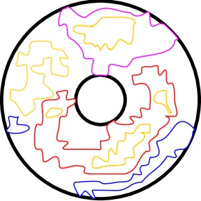
a.   b.

Figure 1: The conformal loop model on the annulus. Different Boltzmann weights are given to the loops, depending on their topology (contractible or not) and if they touch a boundary. There can be a loop touching both boundariers if and only if there is no non-contractible loop (a). There is always an even number of non-contractible loops, and they are allowed to touch the boundaries (b).

This model is endowed with conformal invariance, so we expect its partition function to be invariant under any conformal mapping. In particular we can study the model on a periodic strip of size $L\times N$ ($L$ in the periodic direction), related to the annulus $A=\left\{z\;:\;R_{1}\leq|z|\leq R_{2}\right\}$ by

$$z^{\prime}\rightarrow z=R_{2}\exp\left(i2\pi\frac{z^{\prime}}{L}\right)$$ (1)

The geometry is characterized by the modular parameter

$$q=e^{-\pi\tau}$$ (2)

where $\tau=L/N=2\pi/\log\frac{R_{2}}{R_{1}}$. As a consequence of conformal invariance, the partition function must depend on the Boltzmann weights of the loops and on the modular parameter $q$ only. It is a well-known result that the central charge of the dense loop gas is

$$c=1-\frac{6}{m(m+1)}$$ (3)

where $m$ is related to the Boltzmann weight of the bulk loops $n$ through

$$n=2\cos\gamma\;,\qquad\gamma=\frac{\pi}{m+1},\qquad m>0.$$ (4)

Note that $m$ is not restricted to be an integer. Let us also recall the Kac formula

$$h_{r,s}=\frac{\left[(m+1)r-ms\right]^{2}-1}{4m(m+1)}.$$ (5)

Contractible	Type	Weight	Parametrization
Yes	Bulk	$n$	$n=2\cos\gamma$
Yes	Boundary $1$	$n_{1}$	$\displaystyle n_{1}=\frac{\sin(r_{1}+1)\gamma}{\sin r_{1}\gamma}$,   $r_{1}\in(0,m+1)$
Yes	Boundary $2$	$n_{2}$	$\displaystyle n_{2}=\frac{\sin(r_{2}+1)\gamma}{\sin r_{2}\gamma}$,   $r_{2}\in(0,m+1)$
Yes	Both Boundaries	$n_{12}$	$\displaystyle n_{12}=\frac{\sin(r_{1}+r_{2}+1-r_{12})\frac{\gamma}{2}\sin(r_{1}+r_{2}+1+r_{12})\frac{\gamma}{2}}{\sin r_{1}\gamma\sin r_{2}\gamma}$
No	Bulk	$l$	$\displaystyle l=2\cos\chi$
No	Boundary $1$	$l_{1}$	$\displaystyle l_{1}=\frac{\sin(u_{1}+1)\chi}{\sin u_{1}\chi}$
No	Boundary $2$	$l_{2}$	$\displaystyle l_{2}=\frac{\sin(u_{2}+1)\chi}{\sin u_{2}\chi}$

Table 1: Loop weights and their parametrizations.

Now we are ready to present the main result of this article. In full generality, the partition function of the boundary loop model is given by

$$Z = \frac{q^{-c/24}}{P(q)}\sum_{n\in Z}q^{h_{r_{12}-2n,r_{12}}}$$ (6)

$$+\frac{q^{-c/24}}{P(q)}\sum_{j\geq 1}\sum_{n\geq 0}\frac{\sin(u_{1}+u_{2}-1+2j)\chi\sin\chi}{\sin u_{1}\chi\sin u_{2}\chi}q^{h_{r_{1}+r_{2}-1-2n,r_{1}+r_{2}-1+2j}}$$

$$+\frac{q^{-c/24}}{P(q)}\sum_{j\geq 1}\sum_{n\geq 0}\frac{\sin(-u_{1}+u_{2}-1+2j)\chi\sin\chi}{\sin-u_{1}\chi\sin u_{2}\chi}q^{h_{-r_{1}+r_{2}-1-2n,-r_{1}+r_{2}-1+2j}}$$

$$+\frac{q^{-c/24}}{P(q)}\sum_{j\geq 1}\sum_{n\geq 0}\frac{\sin(u_{1}-u_{2}-1+2j)\chi\sin\chi}{\sin u_{1}\chi\sin-u_{2}\chi}q^{h_{r_{1}-r_{2}-1-2n,r_{1}-r_{2}-1+2j}}$$

$$+\frac{q^{-c/24}}{P(q)}\sum_{j\geq 1}\sum_{n\geq 0}\frac{\sin(-u_{1}-u_{2}-1+2j)\chi\sin\chi}{\sin-u_{1}\chi\sin-u_{2}\chi}q^{h_{-r_{1}-r_{2}-1-2n,-r_{1}-r_{2}-1+2j}}$$

where the seven parameters appearing are fixed by the seven different loop weights. The relations between all these parameters are given in Table 1. Note that $P(q)$ is our notation for $\prod_{k\geq 1}\left(1-q^{k}\right)$.

2 Some algebraic preliminaries

Let us begin by introducing a few algebraic concepts that we will need throughout our discussion. Our model is the densely packed loop model on the tilted square lattice. A very convenient way to think about it is to view it as a face model (see Fig. 2). Each face can be of two different kinds, corresponding to a horizontal or a vertical splitting of the loops.

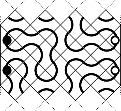
Figure 2: A configuration of dense loops on the tilted square lattice. Loops touching at least once the first (resp. second) boundary are marked with a black (resp. white) blob.

Each closed loop is given a Boltzmann weight $n$. The loops touching the boundaries are distinguished from the bulk ones in our model, and they are given different Boltzmann weights $n_{1}$, $n_{2}$ or $n_{12}$ if they touch the first boundary, the second one, or both of them. The total weight of a particular configuration is then $n^{N}n_{1}^{N_{1}}n_{2}^{N_{2}}n_{12}^{N_{12}}$ where the $N_{i}$’s are the numbers of loops of each kind. We shall later refine these weights to include information about the homotopy class (contractible or not) of each loop.

2.1 The Temperley-Lieb algebra

To begin with, we just drop the distinction of the boundary loops. Then partition function of such a loop model can be reformulated in terms of local operators satisfying some commutation relations that will correctly count the closed loops. The trick is done by the celebrated Temperley-Lieb algebra [TL], defined as follows. The Temperley-Lieb algebra $TL_{N}$ defined on $N$ strands consists of all the words written with the $N-1$ generators $e_{i}$ ($1\leq i\leq N-1$), subject to the relations

$$\left|i-j\right|\geq 2 \Rightarrow e_{i}e_{j}=e_{i}e_{j}$$ (7a)

$$e_{i}^{2} = ne_{i}$$ (7b)

$$e_{i}e_{i\pm 1}e_{i} = e_{i}$$ (7c)

The point of this definition originates in its graphic representation. Represent $e_{i}$ as an operator acting on $N$ strands

$$\underbrace{\begin{pspicture}(-2.84526pt,0.0pt)(19.91692pt,22.76219pt){\psset{}\psline(2.84526pt,0.0pt)(2.84526pt,17.07164pt)}{\psset{}\psline(14.22636pt,0.0pt)(14.22636pt,17.07164pt)}\end{pspicture}\ldots\begin{pspicture}(-2.84526pt,0.0pt)(19.91692pt,22.76219pt)\psellipticarc{-}(0.3,0.)(0.2,-0.25){180}{0}\psellipticarc{-}(0.3,0.6)(0.2,0.25){180}{0}\rput{0.0}(2.84526pt,19.91692pt){${}^{i}$}\rput{0.0}(14.22636pt,19.91692pt){${}^{i+1}$}\end{pspicture}\ldots\begin{pspicture}(-2.84526pt,0.0pt)(19.91692pt,22.76219pt){\psline(2.84526pt,0.0pt)(2.84526pt,17.07164pt)}{\psline(14.22636pt,0.0pt)(14.22636pt,17.07164pt)}\end{pspicture}}_{N}$$

then ($\ref{TLdef}b$)–($\ref{TLdef}c$) read respectively

$$-(0.3,0.)(0.2,-0.25)1800-(0.3,1.2)(0.2,0.25)1800ii+1=n-(0fragments-(0.3,0.)(0.2,-0.25)1800-(0.3,1.2)(0.2,0.25)1800ii+1n-(0$$