A wave effect enabling universal frequency scaling, monostatic passive radar, incoherent aperture synthesis, and general immunity to jamming and interference

ABSTRACT

A fundamental Doppler-like but asymmetric wave effect that shifts received signals in frequency in proportion to their respective source distances, was recently described as means for a whole new generation of communication technology using angle and distance, potentially replacing TDM, FDM or CDMA, for multiplexing. It is equivalent to wave packet compression by scaling of time at the receiver, converting path-dependent phase into distance-dependent shifts, and can multiply the capacity of physical channels. The effect was hitherto unsuspected in physics, appears to be responsible for both the cosmological acceleration and the Pioneer 10/11 anomaly, and is exhibited in audio data. This paper discusses how it may be exploited for instant, passive ranging of signal sources, for verification, rescue and navigation; incoherent aperture synthesis for smaller, yet more accurate radars; universal immunity to jamming or interference; and precision frequency scaling of radiant energy in general.

I Introduction

A previously unsuspected result of the wave equation, enabling a receiver to get frequency shifts in an incoming signal in proportion to the physical distance of its source, was recently described [1]. Its main premise, that signals from real sources must have nonzero spectral spread, seems to be well supported by the cosmological and the Pioneer 10/11 anomalous acceleration datasets, and a remarkably large gamut of terrestrial mysteries that can be mundanely resolved. This perceived support actually concerns a further inference that the mechanism could occur naturally in our instruments on the order of magnitude of $10^{-18}~{}\reciprocal{\mathrm{s}}$. This is a decay corresponding, as half-life, to the age of the solar system, and is too small for purely terrestrial applications. The wave effect is consistently demonstrated with acoustic samples, however, testifying to its fundamental and generic nature. While a general exposition deserves to be made in due course in a physics forum, it presents fundamental new opportunities for intelligence and military technologies.

Section II contains a brief review of the theory of the effect, showing that all real signals necessarily carry source distance information in the spectral distribution of phase, analogous to the ordinary spatial curvature of wavefronts, and that by scanning this phase spectrum, each frequency in a received waveform comprising multiple signals would be shifted in proportion to its own source distance and the scanning rate. Section III presents the general principles of realization by both spectrometry and digital means. Section IV shows how this enables separation of signals by physics instead of modulation, whose implications for information theory have been discussed [ibid.]. Intelligence and military possibilities are considered for the first time in Section V.

II Hubble’s law shifts, temporal parallax

The sole premise for the effect, as mentioned, is the nonzero bandwidth of a real signal. The Green’s function for the general wave equation concerns an impulse function $\delta(\mathbf{x},t)$ as the elemental source. Its Fourier transform is

$$F[\delta(t)]=\int\delta(t)\,e^{-i\omega t}\,dt=1\quad,$$ (1)

which says that all spectral components of an impulse start with the same phase. The source itself is the only common reference across any continuous set of frequencies, hence the spectral phase contours indicate its distance (Fig. 1).

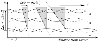
Figure 1: Phase contours and gradient for a source impulse

The main difficulty in tapping this available source of source distance information is that it lies in differences of phase across incoming frequencies, and phases are hard to measure accurately. However, if we scanned the spectrum at rate $d\widehat{k}/dt$, then, for each contour $\phi$ and source distance $r$, we should encounter an increasing or decreasing phase proportional to $r$ and the integration interval $\Delta\widehat{k}$, as shown by the shaded areas in the figure. The trick that yields this remarkable asymmetric effect is in the definition that a rate of change of phase is a frequency, so that the instantaneous measures of the spectral phase contours obtained from the scanning have the form of frequency shifts proportional to the slopes, and therefore to the respective source distances. These distance-dependent shifts resemble Hubble’s law in astronomy but are strictly linear due to their nonrelativistic, mundane origin, and are rigorously predicted by basic wave theory, as follows. The instantaneous phase of a sinusoidal wave at $(\mathbb{r},t)$, from a source at $\mathbf{r}=0$, would be

$$\phi(\mathbf{k},\omega,t)=\mathbf{k}\cdot\mathbf{r}-\omega\;t\quad,$$ (2)

and leads to the differential relation

$$\left.\Delta\phi\right|_{\omega,t}=\Delta(\omega\;t)+\mathbf{k}\cdot\Delta\mathbf{r}+\Delta\mathbf{k}\cdot\mathbf{r}\quad.$$ (3)

The first term $\Delta(\omega\;t)$ clearly concerns the signal content if any, and has no immediate relevance. The second term $\mathbf{k}\cdot\Delta\mathbf{r}$ expresses the path phase differences at any individual frequency, and is involved in the ordinary Doppler effect, as it describes phase change due to changing source distance, as well as image reconstruction in holography and synthetic aperture radar (SAR), as the reconstructed image concerns information of incremental distances of the spatial features of the image. The third term, clearly orthogonal to other two, represents phase differences across frequencies for any given (fixed) source distance. Then, by varying a frequency selection $\widehat{k}$ at the receiver, we should see an incremental frequency, or shift,

$$\delta\omega=\lim_{\Delta t\rightarrow 0}\left[\frac{\left.\Delta\phi(\omega)\right|_{\omega,r,t}}{\Delta k}\times\frac{\Delta\widehat{k}}{\Delta t}\right]=\left.\frac{\partial\phi}{\partial k}\right|_{\omega,r,t}.\frac{d\widehat{k}}{dt}\quad.$$ (4)

(Note that $k$ can only refer to the incoming wave vector in the denominator.) As this holds for each individual $\omega$, from equation (2), the signal spectrum would be uniformly shifted by the normalized shift factor

$$\begin{split}z(r)\equiv\frac{\delta\omega}{\widehat{\omega}}&=\frac{1}{\widehat{\omega}}\left.\frac{\partial\phi}{\partial k}\right|_{\omega,r,t}.\frac{d\widehat{k}}{dt}=\frac{r}{\widehat{k}c}.\frac{d\widehat{k}}{dt}=\frac{\beta r}{c}=\alpha\,r\quad,\\ \text{with}\quad\beta&\equiv\widehat{k}^{-1}(d\widehat{k}/dt)\quad\text{and}\quad\alpha=\beta/c\quad,\end{split}$$ (5)

where $t$ denotes time kept by the receiver’s clock. Further, the shifts reflect only the instantaneous value of $\beta$, which is the normalized rate of change at the receiver.

Fig. 2 shows that $\delta\omega$ is a temporal analogue of spatial parallax, with the instantaneous value of $\alpha\equiv\beta/c$ serving in the role of lateral displacement of the observer’s eyes: at each value $\alpha_{1}$ or $\alpha_{2}$, the signal spectrum $\mathcal{F}(\omega)$ shifts to $\mathcal{F}(\omega_{1})$ or $\mathcal{F}(\omega_{2})$, respectively, and if the distance to the source were increased to $r+\delta r$, the spectrum would further shift to $\mathcal{F}(\omega_{3})$. Unlike with ordinary (spatial) parallax, the receiver can be fixed and monostatic, and yet exploit the physical information of source distance.

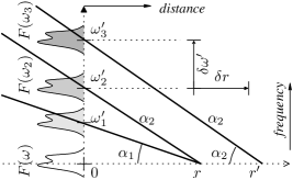
Figure 2: Temporal parallax

III Physics of realization

There are three basic ways of accomplishing Fourier decomposition or frequency selection in a receiver: using diffraction or refraction, a resonant circuit, or by sampling and digital signal processing (DSP). Realization of the shifts in all three methods has been described, along with how this “virtual Hubble” effect had remained unnoticed so long [ibid.]. A review of the diffraction and DSP methods is necessary as theoretical foundation for the application ideas to be discussed. These methods would also be applicable for array antennas and software-defined radio, respectively.

III-A Diffractive implementation

Diffractive selection of a wavelength $\widehat{k}$ concerns using a diffraction grating to deflect normally incident rays to an angle $\theta$ corresponding to the selected $\widehat{k}$, as determined by the grating equation $n\lambda=l\sin\theta$, where $n$ denotes the order of diffraction, and $l$ is the grating interval,

The property exploited is that rays arriving at one end of the grating combine with rays that arrived at the other end a little earlier. If we could change the grating intervals $l$ inbetween, the rays that get summed at a diffraction angle $\theta$ would correspond to changing grating intervals $l(t)$, as depicted in Fig. 3. Their wavelengths must then relate to the grating interval as $n\,d\lambda/dt=(dl/dt)\,\sin\theta$. Upon dividing this by the grating equation, we obtain the modified relation $\widehat{\lambda}^{-1}(d\widehat{\lambda}/dt)=\widehat{l}^{-1}(d\widehat{l}/dt)\equiv-\beta.$

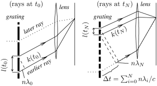
Figure 3: Time-varying diffraction method

This result is not merely a coincidence of different wavelengths at the focal point, as would be obtained with a nonuniform grating. Each of the summed contributions itself has a time-varying $\lambda$, so the variation over the sum is consistent with the component variations. A grating gathers more total power than, say, a two-slit device, and the waves arrive with instantaneously varying phases

$$\frac{d\phi}{dt}\equiv-\widehat{\omega}=\frac{\partial\phi}{\partial t}+\nabla_{\mathbf{r}}\phi\cdot\mathbf{\dot{r}}+\nabla_{\mathbf{r^{\prime}}}\phi\cdot\mathbf{\dot{r}^{\prime}}+\nabla_{\mathbf{k}}\phi\cdot\mathbf{\dot{\widehat{k}}}\quad,$$ (6)

where the first term $\partial\phi/\partial t$ is the signal ($\omega\;t$) contribution in equation (2) and is equal to $-\omega$; the second term (in $\mathbf{\dot{r}}$) concerns the real motion and Doppler effect if any, to be ignored hereon; the third term (in $\mathbf{\dot{r}^{\prime}}$) represents a similar Doppler shift from longitudinal motion of either end of the receiver, which would be generally negligible for $r^{\prime}\ll r$; and only the last term concerns equation (4).

III-B DSP implementation

In DSP, $\widehat{k}$’s are determined by the sampling interval $T$, and can therefore be continuously varied by changing $T$. The discrete Fourier transform (DFT) is defined as

$$\begin{split}F(m\omega_{T})&=\sum_{n=0}^{N-1}e^{im\omega_{T}T}\,f(nT)\\ \text{with the inverse}\quad f(nT)&=\frac{1}{N}\sum_{m=0}^{N-1}e^{im\omega_{T}T}\,F(m\omega_{T})\quad,\end{split}$$ (7)

where $f$ is the input signal; $T$ is the sampling interval; $N$ is the number of samples per block; and $\omega_{T}=2\pi/NT$. The inversion is governed by the orthogonality condition

$$\sum_{n=0}^{N-1}e^{im\omega_{T}T}\,e^{i(kr-n\omega_{T}T)}=\frac{1-e^{i(m-n)}}{1-e^{i(m-n)/N}}=N\delta_{mn}\quad,$$ (8)

where $\delta_{mn}=1$ if $m=n$, else $0$. These definitions as such suggest that the instantaneous selections $\widehat{\omega}_{T}\equiv\widehat{k}c$ can be varied via the sampling interval $T$.

To verify that a controlled variation of $T$ will indeed yield the desired shifts, observe that in equation (6), both the real Doppler terms, in $\dot{\mathbf{r}}$ and $\dot{\mathbf{r}}^{\prime}$, can be ignored, as $r^{\prime}\ll r$ for sources of practical interest. The surviving term on the right is $(\partial\phi/\partial k)(d\widehat{k}/dt)$ where $\partial\phi/\partial t=-\omega$, as before, and

$$\frac{d\widehat{k}}{dt}=\frac{1}{c}\frac{d\widehat{\omega}_{T}}{dt}=\frac{1}{c}\frac{d}{dt}\left(\frac{2\pi}{NT}\right)=-\frac{2\pi}{NcT^{2}}\frac{dT}{dt}=-\widehat{k}\,\frac{1}{T}\frac{dT}{dt}\quad,$$

so that, corresponding to equation (5), we do get

$$\widehat{k}^{-1}(d\widehat{k}/dt)\equiv\beta=-T^{-1}(dT/dt)\quad,$$ (9)

confirming the desired effective variation of $\widehat{k}$’s. $\mathbb{\Box}$

Fig. 4 explains the result. The incoming wave presents increasing phase differences $\delta\phi_{1}$, $\delta\phi_{2}$, $\delta\phi_{3}$, … within the successive samples obtained from the diminishing intervals $\delta T_{1}=T_{1}-T_{0}$, $\delta T_{2}=T_{2}-T_{1}$, $\delta T_{3}=T_{3}-T_{2}$, etc. From the relation $\widehat{\omega}_{T}\equiv\widehat{k}c=2\pi/NT$, gradients of the spectral phase contours can be quantified as

$$\frac{\partial\phi}{\partial T}=\frac{\partial\phi}{\partial\widehat{k}}\frac{d\widehat{k}}{dT}=-\frac{2\pi}{NcT^{2}}\frac{\partial\phi}{\partial\widehat{k}}$$

so that by equation (9), each phase gradient reduces to

$$\frac{\partial\phi}{\partial T}\frac{dT}{dt}=\frac{-2\pi}{NcT}\frac{\partial\phi}{\partial\widehat{k}}\cdot\frac{1}{T}\frac{dT}{dt}=\frac{\widehat{\omega}_{T}}{c}\frac{\partial\phi}{\partial\widehat{k}}\cdot\frac{1}{\widehat{k}}\frac{d\widehat{k}}{dt}=\frac{\partial\phi}{\partial\widehat{k}}\frac{d\widehat{k}}{dt}$$ (10)

identically, validating the approach.

Figure 4: Variable sampling method

III-C General operating principles

For a desired shift $z$ at a range $r$, equation (5) yields

$$\frac{\delta\widehat{k}}{k}\equiv-\frac{\delta{T}}{T}\approx\frac{cz\;\delta t}{r}$$ (11)

for normalized incremental change of the receiver’s grating or sampling interval required over a small interval $\delta t$. In a DSP implementation, appropriate at suboptical frequencies, this determines the needed rate of change over a sampling interval $\delta T$. As $\delta T$ would be nominally chosen based on the (carrier) frequencies of interest and not on the range, the nominal rate of change for achieving a useful $z$ at a given range $r$ would be independent of the operating frequencies.

For example, for a $1~{}\mathrm{G}\mathrm{Hz}$ signal, a suitable choice of sampling interval is $\delta t=100~{}\mathrm{p}\mathrm{s}$, regardless of the range. Chosing $z=2$, which is fairly large in astronomical terms but convenient for the present purposes, we obtain $\delta\widehat{k}/{k}=6\times 10^{-2}/r$ per sample (taking $c=3\times 10^{8}~{}\mathrm{m}\mathrm{/}\mathrm{s}$). At $r=1~{}\mathrm{m}$, the result is a somewhat demanding $6\times 10^{-2}$, or $6\%$, per sample, but for $r=1,~{}10$ or $1000~{}\mathrm{k}\mathrm{m}$, it is $6\times 10^{-5},~{}6\times 10^{-8}$ and $6\times 10^{-11}$ per sample, respectively.

To be noticed is that since equation (11) prescribes a normalized rate of change, the instantaneous rate of change must grow exponentially in the course of the observation, since by integrating equation (11), we get

$$\Delta\widehat{k}\equiv\Delta T^{-1}=e^{cz\Delta t/r},$$ (12)

where $\Delta t$ denotes the total period of observation. While an exponential variation is generally difficult to achieve other than with DSP, two other problems must be also contended with: the total variation over an arbitrarily long observation would be impossible anyway and it could exceed the source bandwidth even over a fairly short observation.

The only solution is to split the observation time into windows, as in DFT, resetting the sampling interval and its variation at the beginning of each window, so that the variation is only continuous within each window.

For example, the normalized rate $6\times 10^{-8}$ calculated above for $100~{}\mathrm{p}\mathrm{s}$ sampling and $10~{}\mathrm{k}\mathrm{m}$ range amounts to $3.773\times 10^{260}$ for each second of observation! Over a $1~{}\mathrm{\SIUnitSymbolMicro}\mathrm{s}$ window, however, the sampling rate would change only by the factor $1.0006$. This is also the spectral spread required of the wavepackets emitted by the source, and conversely, the window can be set to match the spread.

It is possible to cascade multiple stages of gratings or DSP, in order to multiply the magnitude of the shifts. Cascading seems straightforward with optical gratings, but in DSP, as the data stream is already broken up into discrete samples by the first stage, and the sampling interval is to be varied in each successive stage relative to its predecessor, it becomes necessary to interpolate the samples between stages. Interpolation is similarly needed for the reverse shift stage in distance-based signal separation (Section IV-B).

These shifts have been verified only by simulation for electromagnetic waves. For sound data ($c\approx 330~{}\mathrm{m}\mathrm{/}\mathrm{s}$), the software does reveal nonuniform spreading of subbands of acoustic samples, consistent with the likely distributions of their sources. Testing in an adequately equipped sound laboratory, as well as with radio waves, is still needed.

III-D Differential techniques

The effect thus scales well from terrestrial to planetary distances, but the incremental changes required per sample are very small. Errors in these changes, from inadvertent causes including thermal or mechanical stresses, could lead to large errors in distance measurements using the effect. The linearity of the effect can be exploited to offset such errors by differential methods. From equation (5), we have

$$\Delta z=\alpha\Delta r+r\Delta\alpha+o(\Delta r,\Delta\alpha),$$ (13)

relating first order uncertainties. First order error due to an uncertainty $\Delta\alpha$ can be eliminated by measurements using different $\alpha$ and using the differences.

Specifically, an error $\Delta z$ would limit the capability for source separation, presuming $r$ is known. By designing a receiver to depend on the difference between two sets of shifts for the same incoming waves, e.g. by applying the DSP method twice with different values of $\alpha$, a $\Delta z$ error can be eliminated. Conversely, for ranging applications, where $z$ is the measured variable, from $r=z/\alpha$, we get

$$\Delta r=\Delta z/\alpha-r\Delta\alpha+o(\Delta z,\Delta\alpha),$$ (14)

so that the first order error $\Delta r$ can be once again eliminated using differences. This is a temporal form of triangulation, illustrated by the lines for $\alpha_{1}$ and $\alpha_{2}$ that converge at $r$ in Fig. 2. Higher order differences would yield more accuracy.

III-E Phase shifting and path length variation

The main difficulty with the method of Section III-A is ensuring uniformity of the grating intervals even while they are changing. The method is not realizable by acousto-optic cells for this reason. Controlled nonuniform sampling and sample interpolation pose similar difficulties for DSP.

The solution is to instead vary the path length after a fixed grating, say using the longitudinal Faraday effect and circular polarization. As the variation now concerns a bulk property, it would be easier. The proof is straightforward. The analogous simplification for DSP is to modify, instead of the sampling interval $T$, the forward transform kernel to

$$F^{(\omega)}(m\widehat{\omega}_{0})\equiv\sum_{n=0}^{N-1}e^{im\widehat{\omega}(t)T}\,f(nT),\quad\widehat{\omega}(t)=\widehat{\omega}_{0}\,e^{\beta\,nT},$$ (15)

i.e. apply changing phase shifts to the successive samples corresponding to the path length. This is more complex, but avoids interpolation noise and access to the RF frontend.

IV Source separation theory

IV-A Transformation kernel

Fourier theory more generally involves the continuous form of the orthogonality condition (8), given by

$$\int_{t}e^{i\widehat{\omega}t}\,e^{i(kr-\omega t)}\,dt=e^{ikr}\delta(\widehat{\omega}-\omega)\quad,$$ (16)

where $\delta()$ is the Dirac delta function. All of the methods described require continuously varying the mechanism of frequency selection. This is equivalent, in a basic sense, to varying the receiver’s notion of the scale of time, the result being a change of the orthogonality condition to

$$\begin{split}\int_{t}e^{i\widehat{\omega}\Delta(t)}e^{i[kr\Delta(r)-\omega t]}\,dt&=\int_{t}e^{ikr\Delta}\,e^{i(\widehat{\omega}\Delta-\omega t)}\,dt\\ &\equiv e^{ikr\Delta}\,\delta[\widehat{\omega}\Delta-\omega]\quad,\end{split}$$ (17)

where $\Delta\equiv\Delta(r)=(1+\alpha r)$ from equation (5), but is also equivalent to $\Delta(t)=(1+\alpha ct)$, via the relation $c=r/t$.

How did we get to equation (17)? Notice that equation (16) already contains the frequency selection factor $e^{i\widehat{\omega}t}$ – the $\Delta$ in the exponent is the variation of $\widehat{\omega}$ provided by the methods of Section III. The second factor $e^{i[kr\Delta(r)-\omega t]}$ must correspondingly represent the incoming component picked by the modified selector; its only difference from equation (16) is the $\Delta$ multiplying the path contribution to phase, $kr$. Why should this $\Delta$ multiply $kr$ and not $\omega t$? The answer lies in the basic premise of equations (2)-(5) that our receiver manipulates the phase of each incoming Fourier component individually, hence $\omega t$, representing the signal component of the instantaneous phase, is not touched.

The $kr$ term is affected, however, since the summing builds up amplitude at only that value of $k$ which matches $\widehat{\omega}\equiv\widehat{k}c$. This aspect is readily verified by simulation, and it defines a lower bound on the window size (Section III-C) in the optical methods, since the window reset would break the photon integration in a photodetector.

Equation (17) is more general than equation (16), as the latter corresponds to the special case of $\Delta=1$ or $\alpha=0$. This property has a fundamental consequence impacting all of physics and engineering: Since $\alpha$ refers to the physics of the instruments and could be arbitrary small but nonzero, there is fundamentally no way to rule out a nonzero $\alpha$ in any finite local set of instruments. The only way to detect a nonzero $\alpha$ is to look for spectral shifts of very distant objects as a large enough $r$ would yield a measurable $z(r)$.

IV-B Distance division multiplexing™

Almost all the applications to be discussed critically depend on the fundamental separation of sources enabled by the present wave effect. Using the notation of quantum theory, we may denote incoming signals by “kets” $|\rangle$, and the receiver states as “bras” $\langle|$, and rewrite equation (16) as $\langle\widehat{\omega}|\omega,r\rangle=e^{ikr}\langle\widehat{\omega}|\omega\rangle$. Equation (17) then becomes

$$\begin{split}\langle\widehat{\omega},\frac{d\widehat{\omega}}{dt}|\omega,r\rangle&\equiv\langle\widehat{\omega}|H|\omega,r\rangle=e^{ikr\Delta(r)}\,\langle\widehat{\omega}|\frac{\omega}{\Delta(r)}\rangle\\ &=e^{ikr\Delta(r)}\,\delta\left(\widehat{\omega}-\frac{\omega}{\Delta(r)}\right)\quad,\end{split}$$ (18)

where $\langle\widehat{\omega},d\widehat{\omega}/dt|$ and $\langle\widehat{\omega}|$ are the modified and original states of the receiver, respectively. The sampling clock and grating modifications then correspond to the operator $H$

$$H|\omega,r\rangle=e^{ikr\Delta(r)}\,|\frac{\omega}{\Delta(r)}\rangle$$ (19)

of an incoming wave state $|\omega,r\rangle$. These equations attribute the shift to the incoming value $\omega$, instead of to $\widehat{\omega}$ selected instantaneously since for the operator formalism, $\langle\widehat{\omega}|$ must represent an eigenstate resulting from observation.

Equations (5) and (19) both say that as in the Doppler case, the shift is proportional at each individual frequency $\omega$. This also means that the spectrum expands by the factor $\Delta$, as illustrated in Fig. 5 for the case of a common signal spectrum $F(\omega)$ emitted by two sources at distances $r_{1}$ and $r_{2}>r_{1}$, respectively. For a rate of change factor $\alpha$ applied at the receiver, the signals will shift and expand by $\Delta_{1}\equiv(1+\alpha r_{1})$ and $\Delta_{2}\equiv(1+\alpha r_{2})>\Delta_{1}$, respectively.

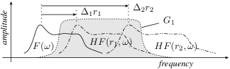
Figure 5: Separation by source distance

Despite the increased spreading of the spectrum, there is opportunity for isolating the signal of a desired source if its shifted spectrum comes out substantially separated from its neighbours, as shown. We could, for instance, apply a band-pass filter $\widetilde{G}_{1}$ to the overall shifted spectrum $HF_{1}+HF_{2}$, such that $\widetilde{G}_{1}(HF_{1}+HF_{2})\approx\widetilde{G}_{1}HF_{1}.$ Writing $H$ as a function of $\alpha$, by equations (17) and (19), we get

$$H^{-1}(\alpha)=-H(\alpha)\quad.$$ (20)

We could apply a combination of mixing and frequency-modulation operations to shift and compress $\widetilde{G}_{1}HF_{1}$ back to $\approx F_{1}(\omega)$, or just apply a second $H$ with a negative $\alpha$. In general, a set of distance-selecting “projection operators” $H^{-1}\widetilde{G}_{i}H$, can thus be defined by the conditions

$$H^{-1}\widetilde{G}_{i}H\,\sum_{j}F(r_{j},\omega)\approx F(r_{j},\omega)\text{~{}or~{}}H^{-1}\widetilde{G}_{i}H\approx\delta_{ij}$$ (21)

With base-band prefilters $G_{i}F_{i}\approx F_{i}$, they yield

$$H^{-1}\widetilde{G}_{i}H=\delta_{ij}G_{j}\quad\text{so that}\quad\widetilde{G}_{i}H=HG_{i}\quad.$$ (22)

As $H$ is parametrized by $\alpha$ independently of $i$, $H\widetilde{G}_{i}H$ provides spectral separation without prior knowledge of $r_{i}$. It is also independent of signal content, wherein the source coordinates could be supplied or included via modulation, but since $H$ depends only on the path phase contribution, it provides separation at a more basic level. Coordinate-based spread spectrum coding could be combined, for example, to differentiate sources at the same distance, as an alternative to or to improve over current phased array antennas.

It has been further suggested [1] that DDM raises the theoretical capacity of a channel to $\sim 2\mathcal{C}L/\lambda\gg\mathcal{C}$, where $\mathcal{C}$ is the traditional Shannon capacity for a source-receiver pair using the channel, by admitting additional sources into the channel at intermediate distances. Further, if combined with directional selectivity say from phased array antennae, we would get true space-division multiplexing [ibid.].

V Military and intelligence applications

The above theory represents a long overdue rigorous analysis of the spectral decomposition of waveforms by a real, and therefore imperfect, instrument. The nature of the error was inferred, as mentioned, from an immense gamut of astronomical, planetary and terrestrial data, spanning all scales of range ever measured. A natural occurrence of the effect subsequently deduced from creep theory (footnote, page 2) could have been contradicted in at least one set of data, but remains totally consistent. Instead, we clearly face a converse problem in physics itself, that its patterns have been so well explored on earth that only astronomical tests can expose remaining shortcomings [5]. The known laws of physics only reflect understood mechanisms, like interference and the Doppler effect and only partially. We once again face a need to lead physics by engineering.

V-A Precision, power-independent frequency shifting

This application would itself be a direct, visible test of the effect, the idea being that the method could be applied also to a proximal source at a precisely known distance in order to uniformly scale its spectrum with great accuracy. Accuracy is expected because the source distance can be accurately set by simple mechanical means, independently of the exponential control of $\alpha$. The mechanism would be the first means for shifting frequencies that is independent of the nature and energy of the waves, and their frequencies and bandwidth, yet realizable by a mundane, static means. The main difficulty is the magnitude of $\alpha$ needed for source distances of under $1~{}\mathrm{m}$, but it should be eventually solvable.

Likely applications include transformation of high power modulated $\mathrm{G}\mathrm{Hz}$ carriers to $\mathrm{T}\mathrm{Hz}$ or optical bands, and efficient, tunable visible light, UV or even X- or $\gamma$-rays, all with controlled coherence and without nonlinear media.

V-B Monostatic ranging and passive radar

This application was immediately envisaged when the effect was first actually suspected, taking from the well known notion of the cosmological distance scale available from the Hubble redshifts. By providing a “virtual Hubble flow” view that can be activated and scaled at the receiver’s discretion, the present methods enable ranging, or distance measurement, of any source that can be seen or received, at only half the round-trip delay, and zero transmitted power.

To compare, as traditional active radar depends on round trip times (RTT), its range is fundamentally limited by the transmitter power. While Venus and Mars have been explored by radar, for example, the ranging of other planets and of astronomical objects in general is largely limited to spatial triangulation, including using the earth’s orbit itself as the baseline. Tracking of orbiting satellites places similar demands on the radar transmitter power $P$, as the range $R$ is governed by the “radar power law” $P\propto R^{4}$. This makes current (active) radars generally bulky. The power law is relaxed for cooperative targets with transponders, to $P\propto R^{2}$, where $P$ denotes transponder power, and the range is obtained from the RTT of a transponded signal. The present methods make this lower power law available for all targets, and also eliminate the need for a spatial baseline for parallax, as the baseline is now given by the range of variation of $\alpha$ at the receiver. As shown in Section III-C, a very large baseline seems to be indeed possible with DSP alone for both terrestrial and earth orbit distances.

Current passive radar technology, like Lockheed’s Silent Sentry, involves coherent processing of the received scatter of energy from television broadcast (see US Patent 3,812,493, 1974) and cellular base stations. The accuracy is again dependent on information representing overall trip times, and hence entails coherent processing.

Accurate ranging is now possible via triangulation using temporal parallax, as explained in Section III-D. The difference is that coherent processing can provide imaging with subwavelength precision, but triangulation would be simpler for ranging and tracking. We still need to illuminate silent targets, but the processing could be simplified for the same accuracy. The accuracy of tracking could improve for radiating targets given the lower overall trip time. We can also use temporal triangulation to simplify traditional radar and as a fast, efficient cross-check.

V-C Overcoming interference, jamming and noise

The capability for separating sources regardless of the signal content or modulation is also a guarantee that a desired signal can be isolated from any interfering signals at the same frequencies and bearing the same modulations or spread-spectrum codes, so long as the interfering sources are at other directions or distances from the receiver.

Simulation shows that even signals in destructive interference can be separated. The criterion for separation is simply the bandwidth to distance ratio: denoting the low and high frequency bounds of the signal bandwidth $W$ by $\mathcal{L}$ and $\mathcal{H}$, respectively, each of equations (5) or (17) implies

$$(1+\alpha r_{i})\mathcal{H}\leq(1+\alpha r_{i+1})\mathcal{L}$$ (23)

as the condition for separation between the $i$th and $(i+1)$th sources, assuming $r_{i}\leq r_{i+1}$ (see Fig. 5). This means

$$\alpha r_{i}\geq\frac{W}{(\delta r_{i}/r_{i})\mathcal{L}-W}=\left[\frac{\delta r_{i}}{r_{i}}\frac{\mathcal{L}}{W}-1\right]$$ (24)

where $W=\mathcal{H}-\mathcal{L}$ and $\delta r_{i}=r_{i+1}-r_{i}$. As separation is only possible for $\alpha>0$, we need to have $\delta r_{i}>r_{i}W/\mathcal{L}$. It then follows, however, that sufficiently narrow subbands of the total received signal would be “source-separable” even when the condition should fail for $W$ as a whole.

All of the limitations are thus purely technological, e.g. how many and how narrow subbands we can construct, how linear we can make the subband and band-pass ($\widehat{G}$) filters (since phase envelope distortions will alter the shift), and how large the stop-band rejection we can get. The stop-band rejection ratio is important in overcoming jamming, and the separation as such should suffice, in principle, for filtering out truly extraneous noise like lightnings.

V-D Incoherent aperture synthesis

In a conventional SAR, multiple targets or features are imaged from the echos received on a moving platform, typically an aircraft or satellite, as depicted in Fig. 6.

Figure 6: Aperture synthesis

If the onboard oscillator could maintain coherence for the duration of the flight, i.e. not suffer random phase shifts, an entire target region could be imaged by a simple Fourier transform, after correcting for the Doppler shifts in the received echos due to the radar’s own motion. At each point $Q$ on the flight path, echos are received from multiple features $A$, $B$, etc. and corresponding to multiple previous locations $P_{1}$, $P_{2}$, … of the transmitter. Fourier techniques and their optical holographic counterparts are most efficient for unravelling the information.

As stated in Section V-B, the fundamental reason for coherent processing is our current dependence on RTT of radar echos for the range information. The dependence is obviated by the wave effect. In the example scenario, echos received at $Q$ from target features differing in direction, like $A$ and $B$, can be separated by the phase information from an antenna array. The echos from the same direction, such as from $A$ and $D$, can now be similarly separated using the methods of Section III – in particular, the changing delay transform of equation (15) can be applied to recordings of the received echo waveform.

Coherent processing ordinarily has two advantages that would seem to be impossible in any other approach: it tends to curtail noise and is generally precise to within a wavelength. We would get suppression of external noise, as discussed in Section V-C, and subwavelength resolution, as shown in Section III-D, so that applications including hand-held short-range carrier-deck operation, for which coherent processing is difficult, become feasible.

References

- [1] V Guruprasad. Relaxed bandwidth sharing with Space Division Multiplexing. In Proceedings of the IEEE Wireless Communication and Networking Conference, March 2005.
- [2] L Parker. Quantized fields and particle creation in expanding universe - I. Phys Rev, 183(5):1057–1068, 25 Jul 1969.
- [3] J D Anderson et al. Study of the anomalous acceleration of Pioneer 10 and 11. Phys Rev D, 65, Apr 2002. Also: report LA-UR-00-5654 and gr-qc/0104064, Apr 2001.
- [4] V Guruprasad (unpublished). astro-ph/9907363 (analysis of the Pioneer 10/11 anomalies, 1999), gr-qc/0005014 (“prediction” of the cosmological acceleration , 2000). At http://www.arxiv.org, both cited in [3].
- [5] J D Anderson et al. Indication from Pioneer 10/11, Galileo and Ulysses data of an apparent anomalous, weak, long-range acceleration. Phys Rev Lett, Oct 1998.
- [6] R P Feynman, R Leighton, and M Sands. The Feynman Lectures on Physics. Addison-Wesley, 1964.
- [7] P L Bender and M A Vincent. Small Mercury Relativity Orbiter. Technical Report N90-19940 12-90, NASA, Aug 1989.
- [8] M A Vincent and P L Bender. Orbit determination and gravitational field accuracy for a Mercury transponder satellite. J Geophy Res, 95:21357–21361, Dec 1990.