Chaos synchronization in networks of coupled maps with time-varying topologies

Abstract

Complexity of dynamical networks can arise not only from the complexity of the topological structure but also from the time evolution of the topology. In this paper, we study the synchronous motion of coupled maps in time-varying complex networks both analytically and numerically. The temporal variation is rather general and formalized as being driven by a metric dynamical system. Four network models are discussed in detail in which the interconnections between vertices vary through time randomly. These models are 1) i.i.d. sequences of random graphs with fixed wiring probability, 2) groups of graphs with random switches between the individual graphs, 3) graphs with temporary random failures of nodes, and 4) the meet-for-dinner model where the vertices are randomly grouped. We show that the temporal variation and randomness of the connection topology can enhance synchronizability in many cases; however, there are also instances where they reduce synchronizability. In analytical terms, the Hajnal diameter of the coupling matrix sequence is presented as a measure for the synchronizability of the graph topology. In topological terms, the decisive criterion for synchronization of coupled chaotic maps is that the union of the time-varying graphs contains a spanning tree.

PACS 05.45.Ra(Coupled map lattices); 05.45.Xt(Synchronization, coupled oscillators); 02.50.Ey(Stochastic processes).

1 Introduction

Synchronization of coupled maps in networks is presently an active research topic [1]. It represents a mathematical framework that on the one hand can elucidate – desired or undesired – synchronization phenomena in diverse applications. On the other hand, the synchronization paradigm is formulated in such a manner that powerful mathematical techniques from dynamical systems and graph theory can be utilized. A standard version of the network of coupled maps, coming from the well-known coupled map lattices (CML) [2], can be formalized as follows:

$$x^{i}(t+1)=f(x^{i}(t))+\sum\limits_{j=1}^{m}L_{ij}f(x^{j}(t)),i=1,\cdots,m,$$ (1)

where $t\in\mathbb{Z}^{+}=\{0,1,2,\cdots,\}$, $x^{i}(t)$ is the state variable of vertex $i$, $f:\mathbb{R}\rightarrow\mathbb{R}$ is a differentiable map, and $L=[L_{ij}]_{i,j=1}^{m}\in\mathbb{R}^{m\times m}$ is the diffusion matrix, which is determined by the topological structure of the network and satisfies $L_{ij}\geq 0$ for all $i\neq j$ and $\sum_{j=1}^{m}L_{ij}=0$ for all $i=1,\cdots,m$. Let $x=[x^{1},x^{2},\dots,x^{m}]^{\top}\in\mathbb{R}^{m}$, $F(x)=[f(x^{1}),f(x^{2}),\dots,f(x^{m})]^{\top}$, and $G=I_{m}+L$, where $I_{m}$ denotes the identity matrix of dimension $m$. Then, Eq. (1) can be rewritten in the matrix form:

$$x(t+1)=GF(x(t))$$ (2)

where $G=[G_{ij}]_{i,j=1}^{m}\in\mathbb{R}^{m\times m}$ denotes the coupling and satisfies $G_{ij}\geq 0$ for $i\neq j$ and $\sum_{j=1}^{m}G_{ij}=1$ for all $i=1,\cdots,m$. Thus, if $G_{ii}\geq 0$ holds for all $i=1,\cdots,m$, then $G$ is a stochastic matrix.

This dynamical system formulation contains two aspects. One of them is the reaction dynamics at each vertex of the network. The other is the coupling structure, that is, whether and how strongly, the dynamics at one vertex is directly influenced by the states of the other vertices. This influence can be described by notions of graph theory. Hence, the coupling matrix $G$ corresponds to a graph $\Gamma=[{\mathcal{V}},{\mathcal{E}}]$, where ${\mathcal{V}}=\{1,2,\cdots,m\}$ denotes the vertex set and ${\mathcal{E}}=\{e_{ij}\}$ denotes the edge set such that there exists a directed edge from vertex $j$ to vertex $i$ if and only if $G_{ij}>0$.

Synchronous dynamics in complex networks have recently attracted increasing attention [1, 3, 4, 5, 6, 7]. Linear stability analysis was used and transverse Lyapunov exponents were introduced to analyze the influence of the topological structure of networks [6]. Ref. [7] has related the ability to synchronize chaotic maps to the existence of a spanning tree in the corresponding graph. However, synchronization analysis has so far been mostly limited to autonomous systems, where the interactions between the state components are static. In [6], a generalized criterion guaranteeing synchronization in the model (2) is proposed as follows:

$$\log|\lambda_{1}|+\mu<0,$$ (3)

where $\mu$ is the Lyapunov exponent of the uncoupled system $s(t+1)=f(s(t))$ and $\lambda_{1}$ is the eigenvalue of the coupling matrix $G$ with the second largest modulus, noting that the largest eigenvalue has a modulus of $1$.

Many real-world applications from the social, natural, and engineering disciplines include a temporal variation of topology of the network. In communication networks, for example, one must consider dynamical networks of moving agents. In this case, some of the existing connections can fail simply due to occurrence of an obstacle between agents [8]. Also, some new connections may be created when one agent enters the effective region of other agents [9, 10, 11]. Furthermore, this temporal variation of topology involves randomness. In [8, 9, 10], consensus in multi-agent networks was considered where the state of each vertex is updated according to the states of its connected neighbors with switching connecting topologies. The consensus protocol of multi-agent dynamical networks can generally be formalized in discrete-time form as

$$x^{i}(t+1)=\sum\limits_{j=1}^{m}G_{ij}(t)x^{j}(t),~{}i=1,\cdots,m,$$ (4)

where $[G_{ij}(t)]_{i,j=1}^{m}$, $t\in\mathbb{Z}^{+}$, are stochastic matrices. It was proved in Ref. [11] that the connectivity of the switching graphs plays a key role in the consensus dynamics of multi-agent networks with switching topologies. Some papers from the recent literature [12] studied synchronization of continuous-time dynamical networks with time-varying topologies; however, the time-varying couplings were specific, with either symmetry, node balance, or fixed time average.

In this paper, we study the local complete synchronization of networks of coupled maps with time-varying couplings:

$$x(t+1)=G(\theta^{(t)}\omega)F(x(t)).$$ (5)

Here, $\theta^{(t)}\cdot$ represents a metric dynamical system $\{\Omega,{\mathcal{F}},P,\theta^{(t)}\}$, where $\Omega$ is the state space, $\mathcal{F}$ is the $\sigma$-algebra, $P$ is the probability measure, and $\theta^{(t)}$ is the semi-flow satisfying $\theta^{(t+s)}=\theta^{(t)}\circ\theta^{(s)}$, where $\theta^{(0)}$ is the identity map, $G(\theta^{(t)}\omega)=[G_{ij}(\theta^{(t)}\omega)]_{i,j=1}^{m}\in\mathbb{R}^{m\times m}$ denotes the coupling matrix at time $t$ and is measurable on $(\Omega,\mathcal{F})$, and $F(x)=[f(x_{1}),\cdots,f(x_{n})]^{\top}$ is a differentiable function.

Thus, Eq. (5) is a random dynamical system. For more details on random dynamical systems, we refer to the textbooks [16]. This form of time-varying coupling is rather general and includes the deterministic case, where $G(\cdot)$ can be regarded as a known function of time $t$, as well as the stochastic case, where $G(\cdot)$ can be regarded as being enforced by a stochastic process $\{\xi^{t}\}_{t\in\mathbb{Z}^{+}}$, namely, $G(\xi^{t})$.

Accordingly, we denote time varying graphs by $\{\Gamma(\theta^{(t)}\omega)\}_{t\in{\mathbb{Z}}^{+}}$. Define $\Gamma(\theta^{(t)}\omega)=[{\mathcal{V}},{\mathcal{E}}(\theta^{(t)}\omega)]$, where ${\mathcal{V}}=\{1,2,\cdots,m\}$ denotes the fixed vertex set and ${\mathcal{E}}(\theta^{(t)}\omega)=\{e_{ij}(\theta^{(t)}\omega)\}$ denotes the edge set of the graph at time $t$, i.e., edge $e_{ij}(\theta^{(t)}\omega)$ exists if and only if $G_{ij}(\theta^{(t)}\omega)>0$. So, the coupling matrix $G(\theta^{(t)}\omega)$ might be a function of the coupling graph topology.

Local complete synchronization (synchronization for short) is defined in the sense that the differences between states of vertices of the coupled dynamical system (5) converge to zero whenever the initial state of each vertex is picked sufficiently near the attractor of the uncoupled system and their differences are sufficiently small, i.e.,

$$\lim_{t\rightarrow\infty}\|x^{i}(t)-x^{j}(t)\|=0,~{}i,j=1,\cdots,m.$$ (6)

For a more geometric definition, suppose that the uncoupled system $s(t+1)=f(s(t))$ possesses an attractor (see Ref. [17] for details), which we denote by $A$. Define

$${\mathcal{S}}=\big{\{}[x^{1},x^{2},\cdots,x^{m}]^{\top}\in\mathbb{R}^{m}:~{}x^{i}=x^{j},~{}i,j=1,\cdots,m\big{\}}$$

which is an invariant subspace of Eq. (5). Let $A^{m}$ denote the Cartesian product $A\times\cdots\times A$ ($m$ times). We define the synchronization manifold by the set $\mathcal{A}=\mathcal{S}\cap A^{m}=\{[x,\cdots,x]:x\in A\}$. In this sense, synchronization is equivalent to the stability of $\mathcal{A}$.

The purpose of this paper is to study the synchronization of the coupled map network (5) with time-varying topology. Here, the topology is generally supposed to be driven by a metric dynamical system and the coupled network can be regarded as a random dynamical system. We present sufficient conditions guaranteeing synchronization. Furthermore, we show that the property that the union of the time-varying graphs contains a spanning tree is very important for the network’s ability to synchronize chaotic maps. Additionally, we present several time-varying network models and study the synchronization of coupled maps on these dynamical networks. The topological structures of these models vary in time and include randomness. Generally, the collections of interconnections in these networks can be regarded as Markov chains. Besides illustrating the theoretical results, we also focus on the variation of synchronizability of each model, which is quantitatively measured with respect to several parameters in the model. As we show, temporal variation and randomness can enhance synchronization in some cases. Further examples indicate that the communication between vertices in the dynamical networks might play an important role in synchronizability.

2 Theoretical analysis

In this section, we present theoretical results on synchronization of coupled map networks with time-varying couplings. The mathematical results have been proven in detail in our companion papers [14, 15]. Our main tool to investigate the synchronous motion of the coupled system (5) is the Hajnal diameter, which was first introduced in Ref. [13] to describe the compression rate of a stochastic matrix and is defined as follows:

Definition 1

For a matrix $G$ with row vectors $g_{1},\cdots,g_{m}$ and a vector norm $\|\cdot\|$ in $\mathbb{R}^{m}$, the Hajnal diameter of $G$ is defined as

$${\rm diam}(G)=\max\limits_{i,j}\|g_{i}-g_{j}\|.$$ (7)

From this definition, synchronization of the coupled system (5) can equivalently be stated as

$$\lim_{t\rightarrow\infty}{\rm diam}([x_{1}(t),\cdots,x_{m}(t)]^{\top})=0.$$ (8)

We can extend this concept to matrix sequences driven by a dynamical system: ${\mathcal{G}}(\omega)=\{G(\theta^{(t)}\omega)\}_{t\geq 0}:\Omega\rightarrow 2^{\mathbb{R}^{m,m}}$ for any $\omega\in\Omega$, where $2^{\mathbb{R}^{m,m}}$ denotes the set composed of all subsets of $\mathbb{R}^{m,m}$. For a matrix sequence ${\mathcal{G}}$, its Hajnal diameter at initial data $\omega\in\Omega$ is defined by

$${\rm diam}(\mathcal{G}(\omega))=\overline{\lim\limits_{t\rightarrow\infty}}\big{\{}{\rm diam}\bigg{[}\prod\limits_{k=0}^{t-1}G(\theta^{(k)}\omega)\bigg{]}\big{\}}^{\frac{1}{t}},$$ (9)

where $\prod$ denotes the left matrix product: $\prod_{k=1}^{n}A_{k}=A_{n}\times A_{n-1}\times\cdots\times A_{1}$. One can see that ${\rm diam}(\mathcal{G}(\omega))<0$ implies that the differences between rows of the infinite matrix product $\prod_{t=0}^{\infty}G(\theta^{(t)}\omega)$ converge to zero as $t$ goes to infinity.

Let $s(t)$ be the synchronized state solution satisfying $s(t+1)=f(s(t))$ for all $t\geq 0$. Let $\delta x(t)=x(t)-s(t)$. Linearizing the system (5) about $s(t)$ gives

$$\delta x(t+1)=f^{\prime}(s(t))G(\theta^{(t)}\omega)\delta x(t).$$ (10)

Note that

$${\rm diam}\bigg{[}\prod\limits_{k=0}^{t-1}G(\theta^{(k)}\omega)f^{\prime}(f^{(k)}(s_{0}))\bigg{]}$$

$$={\rm diam}\bigg{[}\prod\limits_{k=0}^{t-1}G(\theta^{(k)}\omega)\bigg{]}\bigg{|}\prod\limits_{l=0}^{t-1}f^{\prime}(f^{(l)}(s_{0}))\bigg{|}.$$ (11)

Then, the Hajnal diameter of the variational system (10) equals to ${\rm diam}({\mathcal{G}}(\omega))e^{\mu}$, where $\mu$ denotes the maximum Lyapunov exponent of the attractor $A$ of the uncoupled system,

$$\mu=\max\limits_{s_{0}\in A}\overline{\lim\limits_{t\rightarrow\infty}}\frac{1}{t}\sum\limits_{k=0}^{t-1}\log|f^{{}^{\prime}}(f^{(k)}(s_{0}))|.$$ (12)

This leads to the following condition

$${\rm diam}(\mathcal{G}(\omega))e^{\mu}<1,$$ (13)

which guarantees that the variable vector $x(t)$ can be synchronized by picking the initial data of $\theta^{(t)}\cdot$ as $\omega$.

Similar to the case of static network topology, we can extend the transverse Lyapunov exponent for the matrix sequence $\mathcal{G}$ in direction $v\in\mathbb{R}^{m}$ as:

$$\sigma(\mathcal{G},\omega,v)=\overline{\lim\limits_{t\rightarrow\infty}}\frac{1}{t}\log\bigg{\|}\prod\limits_{k=0}^{t-1}G(\theta^{(k)}\omega)v\bigg{\|}$$ (14)

Along the synchronization direction $e_{0}=[1,1,\cdots,1]^{\top}$,
one has $\sigma(\mathcal{G},\omega,e_{0})=0$ since $G(\cdot)$ has a common row sum of unity. Let $0=\sigma_{0}\geq\sigma_{1}\geq\sigma_{2}\geq\cdots\geq\sigma_{m}$ be the Lyapunov exponents for the initial condition $\omega$, counted with multiplicities. We have $\sigma_{1}(\omega)=\log{\rm diam}(\mathcal{G}(\omega))$ according to lemma 2.7 in Ref. [14]. Then, the condition (13) can be rewritten as

$$\sigma_{1}+\mu<0.$$ (15)

If (15) is satisfied, then the coupled system (5) can synchronize.

Remark 1

By Proposition 4.4 in Ref. [14], one can see that the criterion (3) for static networks is a direct consequence of the criterion (15).

We apply the above results to the case where the time-varying coupling is induced by a homogeneous Markov chain $\{\sigma^{t}\}_{t\in\mathbb{Z}^{+}}$ defined on a finite state space with an irreducible transition probability matrix. Also, a homogeneous Markov chain can be regarded as a dynamical system $(\Omega,\mathcal{F},P_{\pi},\theta^{(t)}\cdot)$ as described in the appendix. We now consider a coupled map network with Markov jump topologies:

$$x^{i}(t+1)=\sum\limits_{j=1}^{m}G_{ij}(\sigma^{t})f(x^{j}(t)),~{}i=1,\cdots,m$$ (16)

or in matrix form:

$$x(t+1)=G(\sigma^{t})F(x(t)).$$ (17)

Results in Ref. [15] indicate that in this case, $\log{\rm diam}(\mathcal{G}(\omega))=\sigma_{1}(\omega)$ exists and is a non-random number for almost every $\omega\in\Omega$. Hence for simplicity we can write ${\rm diam}(\mathcal{G}(\omega))$ as ${\rm diam}(\mathcal{G})$ and $\sigma_{1}(\omega)$ as $\sigma_{1}$. From (13), one can obtain the criterion for synchronization of coupled maps (17) as

$$\log{\rm diam}(\mathcal{G})+\mu<0.$$ (18)

According to the equivalence, we can rewrite the condition (18) as the inequality (15). From the criteria (18)–(15), the Hajnal diameter ${\rm diam}(\mathcal{G})$, or equivalently, $\sigma_{1}$, can be used to measure the synchronizability of a Markov jump graph topology process. The question then arises under what conditions this graph process can synchronize some chaotic dynamics, i.e., when does it hold that ${\rm diam}(\mathcal{G})<1$. The following result comes from Theorem 4.2 in Ref. [14] and the theory of Markov chains [21].

Theorem 1

Suppose that $G(\cdot)$ has all diagonal elements positive and the transition probability matrix $T$ is irreducible. Then, ${\rm diam}(\mathcal{G})<1$ if and only if the graph union $\bigcup_{i\in\underline{N}}\Gamma(i)$ possesses a spanning tree.

For the detailed proof, we refer to Ref. [15]. This theorem shows that there exist cases when a Markov jump graph process can synchronize a chaotic map (with $\mu>0$) even though at each instant the network may be disconnected, as long as the union graph has a spanning tree.

3 Applications

In the following, we will study the synchronous dynamics in four time-varying graph process models. In each model, the number of vertices is constant in time but the interconnections between vertices vary, and the variation of interactions can be regarded as a Markov chain. We expect, on the one hand, to illustrate the theoretical results of the previous section, and on the other hand, to numerically analyze the synchronizability as computed by the largest nonzero Lyapunov exponent $\sigma_{1}$, by observing the variations of $\sigma_{1}$ with respect to several parameters in the models.

The map $f$ is chosen here as the logistic map: $f=ax(1-x)$. We take the parameter $a=3.90$ throughout this section (hence with the Lyapunov exponent $\mu\approx 0.5$). Thus, we can focus on the influence of the time-varying coupling on synchronous motions by fixing the parameter of the coupled map, which fixes the Lyapunov exponent $\mu$ of the uncoupled system. (Note that the theoretical results presented above do not depend on this particular choice of chaotic dynamics.)

We realize the coupled networks via two types of coupling configurations. The first system is the coupled map lattice via a time varying graph process:

$$x^{i}(t+1)=\left\{\begin{array}[]{l}f(x^{i}(t))+\displaystyle{\frac{\epsilon}{k_{i}(t)}}\sum\limits_{j=1}^{m}A_{ij}(t)[f(x^{j}(t)-f(x^{i}(t)],~{}~{}~{}\text{if }k_{i}(t)>0,\\ f(x^{i}(t)),~{}~{}~{}~{}~{}~{}~{}~{}~{}~{}~{}~{}~{}~{}~{}~{}~{}~{}~{}~{}~{}~{}~{}~{}~{}~{}~{}~{}~{}~{}~{}~{}~{}~{}~{}~{}~{}~{}~{}~{}~{}~{}~{}~{}~{}~{}~{}~{}~{}~{}\text{if }k_{i}(t)=0,\end{array}\right.$$ (19)

where $i=1,\cdots,m$, $\epsilon\geq 0$ is the coupling strength, $A(t)$ denotes the adjacency matrix of the graph at time $t$, and $k_{i}(t)=\sum_{j\neq i}A_{ij}(t)$ denotes the (in-)degree of vertex $i$ at time $t$. Synchronization is measured by the time average of the variance of the states over the network:

$$K=\bigg{\langle}\frac{1}{m-1}\sum_{i=1}^{m}[x^{i}(t)-\bar{x}(t)]^{2}\bigg{\rangle},$$

where $\bar{x}=(1/m)\sum_{i=1}^{m}x^{i}(t)$ and $\langle\cdot\rangle$ denotes the time average. One can regard $K$ as a function of the coupling strength $\epsilon$. Let $[G(t)]_{ij}=\delta_{ij}(1-\epsilon)+\epsilon k_{i}^{-1}(t)[A(t)]_{ij}$ if $k_{i}(t)>0$ and $[G(t)]_{ij}=\delta_{ij}$ otherwise, where $\delta_{ij}$ are the elements of the identity matrix $I_{m}$. Then, the second largest Lyapunov exponent $\sigma_{1}$ of the stochastic matrix series $\{G(t)\}_{t\in{\mathcal{Z}}^{+}}$ is also a function of $\epsilon$. We also define $W=\sigma_{1}+\mu$, which is the largest Lyapunov exponent of the system (19) in directions transverse to the synchronization manifold.

The second system is the dynamical multi-agent system with the logistic output function $f$ given above. At each vertex $i$, the state is the average of the values $f(x^{i}(t))$ of all its neighbors and itself, i.e.,

$$x^{i}(t+1)={\displaystyle\frac{1}{k_{i}(t)+1}}\bigg{[}\sum\limits_{j\in{\mathcal{N}}_{i}(t)}f(x^{j}(t))+f(x^{i}(t))\bigg{]},~{}~{}~{}~{}~{}i=1,\cdots,m,$$ (20)

where ${\mathcal{N}}_{i}(t)$ denotes the neighborhood of vertex $i$ in graph $\Gamma(t)$ and $k_{i}(t)$ is the degree of the vertex $i$ at time $t$. So, $G_{ij}(t)=1/(k_{i}(t)+1)$ in the form (5) if vertex $j$ is linked to vertex $i$ at time $t$; otherwise, $G_{ij}=0$. According to the criterion (15), the quantity $\sigma_{1}$ can be utilized to measure synchronizability of the time varying graph process of the coupled system (20). A smaller value of $\sigma_{1}$ indicates better synchronizability. The simulation time length is $1000$ in all cases.

3.1 I.i.d. random graphs

In the independent-identical-distribution (i.i.d.) random graph, the edge for each pair of vertices can disappear or appear randomly, independent of time and other pairs of vertices and following an identical distribution. This is a special case of the model introduced in Ref. [9]. As a realization in the present paper, at each time $t$, $\Gamma(t)$ is a $p$-random graph following the famous Erdös-Renyi model [22]: for every pair $(i,j)$, we randomly put an edge between them with probability $p$ and the selection is statistically independent for different times $t$ and other pairs of vertices.

We realize the coupled map networks (19) and (20) in this model. Figure 1 (a) indicates that the parameter range of the coupling strength $\epsilon$ for which synchronization occurs coincides with the range where $W(\epsilon)<0$. This verifies the criterion (15). From the criterion (3), the synchronizability measure for static networks is $\log|\lambda_{1}|$, which has been studied in e.g. Ref. [27]. From figure 2 (a), we observe the variation of $\sigma_{1}$ with respect to $p$ and compare it to the logarithm of the second largest eigenvalue (in modulus) of the coupling matrix of the static random graph in the coupled model (20). One can see that the synchronizability of i.i.d. random graphs increases with increasing probability parameter $p$ and is clearly better than a static random graph of the same size and with the same wiring probability $p$. This implies that in a random network, temporal variation and randomness can increase synchronizability. Furthermore, as one would expect, synchronizability increases with the wiring probability $p$.

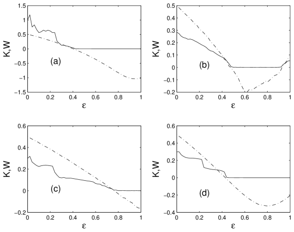
Figure 1: Variation of $K$ and $W$ with respect to $\epsilon$. Figures (a)-(d) are plotted for coupled logistic maps (19). (a) i.i.d. random network with $200$ vertices and $p=0.1$; (b) networks with switching topologies between $\Gamma_{3}$ and $\Gamma_{4}$ with switching probability $p=0.5$; (c) random error model: beginning with a scale-free network introduced in [24] with $200$ vertices and average degree $20$, failure occurs with probability $p=0.01$ and the recovery time $T=3$; (d) meet-for-dinner model with $N=200$ members and subgroups of size $n=5$ . In all cases, $K$ is shown by solid lines ($-$) and $W$ is shown by dotted lines ($-\cdot-$).

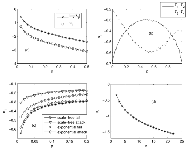
Figure 2: Synchronizability of different graph processes. Subfigures (a)-(d) are plotted for the variation of synchronizability $\sigma_{1}$ with respect to the parameters of the coupled network (20). (a) The variation of $\sigma_{1}$ of an i.i.d. random network with respect to the parameter $p$ and $\log|\lambda_{1}|$ where $\lambda_{1}$ is the second largest eigenvalue of the coupling matrix of a static random graph with the same $p$ in the model (20). The network size is 1024. (b) The variation of $\sigma_{1}$ of a randomly switching network with respect to $p$, for the first group $\{\Gamma_{1},\Gamma_{2}\}$ and the second group $\{\Gamma_{3},\Gamma_{4}\}$ of Figure 3. (c) The variation of $\sigma_{1}$ of malfunction-and-recovery networks with respect to malfunction fraction $p$, with recovery time $T=5$, for failure and attack on scale-free and random networks. The initial scale-free network has size $N=1024$ and average degree $20$, and the random network has $N=1024$ and average degree $152$. (d) The variation of $\sigma_{1}$ of the meet-for-dinner model with respect to $n$, in a network of size $N=1024$.

3.2 Randomly switching topologies

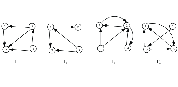
Figure 3: Two groups of graphs $\{\Gamma_{1},\Gamma_{2}\}$ and $\{\Gamma_{3},\Gamma_{4}\}$. Switch occurs in either group randomly. Namely, at each time, with probability $p$ the graph topology is selected as $\Gamma_{1}$ (respectively, $\Gamma_{3}$) and with probability $1-p$ as $\Gamma_{2}$ (resp., $\Gamma_{4}$).

Randomly switching topologies were introduced in Ref. [8]. That is, the graph topology at time $t$ is randomly picked from a given finite set of topologies that follows an identical time-independent distribution. Here, we consider two pairs of graphs, see $\{\Gamma_{1}$, $\Gamma_{2}\}$ and $\{\Gamma_{3}$, $\Gamma_{4}\}$ in figure 3. The random switch occurs between the two graphs of each pair. The switching signal is driven by a Bernoulli random variable $v$. For some constant $p\in(0,1)$, if $v<p$ then the first graph in each pair is chosen as the coupling topology; otherwise, the second graph is chosen.

From figure 1 (b), one can see that the parameter region for which $\sigma_{1}+\mu<0$ equals to the region where $K\approx 0$, which verifies the criterion (15). From figure 2 (b), one can see that for the graph pair $\{\Gamma_{1},\Gamma_{2}\}$, the synchronizability of random switching measured by $\sigma_{1}$ is worse than either of the individual graphs (noting that the synchronizability of each graph can be found at the endpoints $p=0$ and $p=1$). In contrast, for the graph pair $\{\Gamma_{3},\Gamma_{4}\}$, the synchronizability obtained by random switching is better than those of the individual graphs. That is to say, there exist instances where temporal variation of the network topology can increase or decrease synchronizability.

3.3 Random errors

In this model, we consider a network with random errors. If an error occurs at a vertex, then all connections of this vertex disappear. This model is characterized by two kinds of errors. One is called failure, which happens to vertices following the uniform distribution; the other is called attack, which happens to vertices following a selective distribution according to a certain statistical property of the vertices. As shown in Ref. [23], for a class of complex networks with inhomogeneous degree distribution (for example, the Barabási-Albert (BA) model), the statistics such as shortest-path diameter and clustering can have good error tolerance if the errors occur as failure but they are extremely vulnerable for attacks based on highest degrees. As shown in Ref. [25], the synchronizability of a network measured by the eigenratio of the corresponding Laplacian almost does not vary if a vertex is randomly removed but dramatically varies by the selective removal of one vertex. In the present paper, we realize attack according to the connection degree of each vertex. Namely, errors happen merely on vertices with highest degrees. In addition, we add a recovery phase: Every malfunctioned vertex will recover, i.e., all its connections will appear, after a fixed time period. We denote by $p$ the fraction of error vertices in the whole vertex set, i.e., there are $\lfloor N\times p\rfloor$ error vertices, where $\lfloor\cdot\rfloor$ denotes the floor function and $N$ is the size of the whole network.

Comparing the regions of the coupling strength where $K\approx 0$ and $W<0$ in figure 1 (c), one can similarly see that the inequality (15) can precisely predict synchronization. Figure 2 (c) indicates the variation of the synchronizability with error occurrence. We use two network models, namely the Barabási-Albert (BA) network introduced in Ref. [24] as a scale-free network (which has a power-law degree distribution $P(k)\sim k^{-\gamma}$, with $\gamma=3$ independent of the size of the network in case of sufficiently large network sizes), and a random network with exponential tails introduced in Ref. [22]. One can see that for a random network with high degrees, owing to the homogeneity of the network, there is no substantial difference in synchronizability whether the malfunctioned vertices are selected randomly or in decreasing order of connection degree. On the other hand, a drastically different behavior is observed for the scale-free network. If the vertices with higher degrees are attacked, the synchronizability is much reduced compared to the case with random failure. Due to the degree inhomogeneity of the BA networks, the vertices with a high degree play a more important role in synchronization than those with smaller degrees.

3.4 Meet for dinner

In the meet-for-dinner model introduced in [26], a group of friends decide to meet for dinner at a particular restaurant but fail to specify a precise time. On the afternoon of the dinner appointment, they need to find a solution to decide on the meeting time. A centralized solution is to have an advanced conference for the whole group; however, if this option is unavailable, then a decentralized solution is that one meets, one at a time, a subset in the subgroup to collect the information of this subgroup about their expected meeting time, and update with this information until obtaining consensus. Here, we set up the model as follows. The whole group has $N$ members. At each time interval, the group is randomly divided into subgroups with $n$ members (if $N\neq 0\mod n$, then we put the remaining ones into the last subgroup) and each subgraph is a complete graph. Furthermore, every division is stochastically independent of each other.

The region of the coupling strength for synchronization coincides with the range where $W<0$ in figure 1 (d). (The tiny region of apparent discrepancy near $\epsilon\approx 0.45$ is an artifact of plotting the curves with finite data points.) Interestingly, the meet-for-dinner model can synchronize a chaotic map $f$ despite the fact that the graph is disconnected at any time. For a static disconnected graph, there exist several vertices whose dynamical information never reaches the others; so, obviously, a chaotic map cannot be synchronized by a disconnected graph. However, if the graph topology is time-varying, despite the disconnectedness of the network at each time, the dynamical information can reach others in a certain time period. Therefore, in this sense, theorem 1 implies that in some cases, temporal variation of the network topology can enhance synchronization. Figure 2(d) shows that the synchronizability of the meet-for-dinner model increases with size $n$ of the subgroups.

4 Conclusions

In conclusion, we have presented an effective method based on the extended Hajnal diameter for matrix sequences to study the synchronization in networks of coupled maps with time varying topologies. As shown by the sufficient criteria guaranteeing synchronization, the Hajnal diameter of the coupling matrix sequence can be utilized to measure network synchronizability. As shown in Sec.3, synchronizability varies with respect to several parameters in time-varying network models. An intuitive interpretation is that the time-cost of communication between vertices might play a key role for synchronization of a dynamical network. The vertices in the i.i.d. random graphs have a higher chance to access others than in a static random graph. Attack to a network with a power-law degree distribution is more likely to interrupt the communication between vertices than random failures. However, for a random network with high average degree, attack and failure can cause almost equal damage in communication between vertices. When the network size increases, the indirect communication of two vertices can be enhanced by the time-varying connection structure, which can increase synchronizability. These phenomena imply that in some cases time-variance and randomness can enhance synchronizability. However, as shown in figure 2 (b), it is also possible to have decreased synchronizability. This issue deserves further investigation in the future.

Appendix: Homogeneous Markov chain with finite state space

A homogeneous Markov chain with finite state space and an irreducible probability transition matrix can be regarded as a metric dynamical system with invariant probability $\{\Omega,\mathcal{F},P,\theta^{(t)}\cdot\}$. Its state space $\Omega={\underline{N}}^{\mathbb{Z}^{+}}$ is composed of all sequences: $\omega=\{\sigma^{t}\}_{t\geq 0}$; its Borel $\sigma$-algebra $\mathcal{F}=\mathcal{B}^{\mathbb{Z}^{+}}$, where $\mathcal{B}$ denotes all subsets of $\underline{N}$, has a basis of the form $\{\sigma^{t_{1}}\in B_{1},\cdots,\sigma^{t_{r}}\in B_{r}\}$ for some $t_{1}\leq t_{2}\leq\cdots\leq t_{r}$ and $B_{l}\in\mathcal{B}$ for all $l=1,\cdots,r$; $\theta$ denotes the shift map, $\theta\omega=\{\sigma^{(t)}\}_{t\geq 1}$; $P_{\pi}$ denotes the probability measure induced by the unique invariant class of the transition probability matrix $\pi$, which is given by

$$P_{\pi}(\sigma^{t_{1}}\in B_{1},\cdots,\sigma^{t_{r}}\in B_{r})=\sum\limits_{i_{l}=1:l,~{}i_{l}\notin\mathbb{T}}^{N}\sum\limits_{i_{t_{l}}\in B_{l}:l=1,\cdots,r}\pi_{i_{1}}t_{i_{1}i_{2}}t_{i_{2}i_{3}}\cdots t_{i_{t_{r-1}}t_{r}},$$ (21)

where $\mathbb{T}=\{t_{1},\cdots,t_{r}\}$, and invariant through $\theta^{(t)}\cdot$. Induced by different initial distributions $\xi$, this system can have different probability measures $P_{\xi}$, but they all are not invariant over $\theta^{(t)}\cdot$. If the invariant probability $\pi$ is ergodic in the sense that each $\pi_{k}>0$, then for any initial distribution $\xi$, $P_{\xi}$ is absolutely continuous with $P_{\pi}$, i.e, $P_{\xi}\ll P_{\pi}$, which implies that any characteristic in the $P_{\pi}$ almost sure sense certainly holds in the almost sure sense for any $P_{\xi}$ if $\pi$ is ergodic, or equivalently, if the transition probability matrix $T$ is irreducible. In this paper, we only focus on the probability measure $P_{\pi}$ and simplify $P_{\pi}$-almost surely by “almost surely” unless denoted otherwise. By the multiplicative ergodic theorem for random dynamical systems [16], the multiplicative Lyapunov exponents for the infinite matrix sequence $\prod_{t=0}^{\infty}G(\sigma^{t})$ exist and are non-random almost surely.

References

- [1] J. Jost, M. P. Joy, Phys. Rev. E 65, 016201 (2001); Y. H. Chen, G. Rangarajan, M. Ding, Phys. Rev. E 67, 026209 (2003); W. Lu, T. Chen, Physica D 198, 148 (2004); R. E. Amritkar, S. Jalan, C-K. Hu, Phys. Rev. E 72, 016212 (2005)
- [2] K. Kaneko, Prog. Theor. Phys. 74, 1033 (1985); T. Bohr, O. B. Christensen, Phys. Rev. Lett. 63, 2161 (1989); K. Kaneko, Theory and Applications of Coupled Map Lattices, (Wiley, New York, 1993)
- [3] A. Pikovsky, M. Rosenblum, J. Kurths, Synchronization: A universal concept in nonlinear sciences (Cambridge University Press, 2001)
- [4] S. Morita, Phys. Rev. E 58, 4401 (1998); A. M. Batista, S. E. de. S. Pinto, R. L. Viana, S. R. Lopes, Phys. Rev. E 65, 056209 (2002)
- [5] T. Shinbrot, Phys. Rev. E 50, 3230 (1994); Y. Jiang, P. Parmananda, Phys. Rev. E 57, 4135 (1998); P. M. Gade, C-K. Hu, Phys. Rev. E 65, 6409 (2000)
- [6] L. M. Pecora, T. L. Caroll, Phys. Rev. Lett. 80, 2109 (1998); G. Rangarajan, M. Ding, Phys. Lett. A 296, 204 (2002); F. M. Atay, T. Biyikoglu, J. Jost, Physica D 224, 35 (2006)
- [7] C. W. Wu, Nonlinearity 18 1057 (2005); W. Lu, T. Chen, IEEE T. CAS:-II 54:2, 136 (2007)
- [8] R. Olfati-Saber, R. M. Murray, IEEE T. Autom. Control 49:9, 1520 (2004)
- [9] Y. Hatano, M. Mesbahi, IEEE Trans. Autom. Control 50:11, 1867 (2004)
- [10] T. Vicsek, A. Czirok, E. B. Jacob, I. Cohen, O. Schochet, Phys. Rev. Lett. 75, 1226 (1995); A. Jadbabaie, J. Lin, A. S. Morse, IEEE T. Autom. Control 48, 988 (2003).
- [11] L. Moreau: IEEE Trans. Autom. Control, 50:2, 169 (2005)
- [12] J. H. Lü, G. Chen, IEEE Trans. Autom. Control 50, 841 (2005); I. V. Belykh, V. N. Belykh, M. Hasler, Physica D 195, 159 (2004); D. J. Stilwell, E. M. Bollt, D. G. Roberson, SIAM J. Appl. Dyn. Syst., 5:1, 140 (2006); S. Boccaletti, D.-U. Hwang, M. Chavez, A. Amann, J. Kurths, L. M. Pecora, Phys. Rev. E 74, 016102 (2006)
- [13] J. Hajnal, Proc. Camb. Phil. Soc. 54, 233 (1958); J. Hajnal, Proc. Camb. Phil. Soc. 52, 67 (1956)
- [14] W. Lu, F. M. Atay, J. Jost, SIAM Journal on Math. Anal. 39, 1231–1259 (2007)
- [15] W. Lu, F. M. Atay, J. Jost, Synchronization in coupled map networks with uncertain topologies (in preparation)
- [16] L. Arnold, Random Dynamical Systems, (Springer-Verlag, Heidelberg, 1998); M. Dunford, J. T. Schwartz, Linear Operators, (Interscience, New York, 1958)
- [17] P. Ashwin, J. Buescu, I. Stewart, Nonlinearity 9, 703–737 (1996)
- [18] J. Milnor, Commun. Math. Phys. 99, 177 (1985)
- [19] L. Arnold, J. Diff. Equ. 177, 235 (2001)
- [20] J. Shen, Wavelet Anal. Multi. Meth. LNPAM, 212, 341 (2000)
- [21] Y. Fang, Ph.D. thesis, Case Western Reserve University, 1994
- [22] P. Erdös, A. Rényi, Publ. Math. Debrecen 6, 290 (1959)
- [23] R. Albert, H. Jeong, A.-L. Barabási, Nature, 406:27, 378 (2000)
- [24] A.-L. Barabási, R. Albert, Science 286, 509 (1999)
- [25] H. Hong, B. J. Kim, M. Y. Choi, H. Park, Phys. Rev. E 69, 067105 (2004)
- [26] W. Ren, R. W. Beard, T. W. McLain, Springer-Verlag Series: LNCIS 309, 171 (2004)
- [27] F. M. Atay, T. Biyikoglu, Phys. Rev. E 72, 016217 (2005) ; F. M. Atay, T. Biyikoglu, J. Jost, IEEE Trans. Circ. Syst.-I 53:1, 92 (2006); F. M. Atay, T. Biyikoglu, J. Jost, Physica D 224, 35 (2006)