We explore electron transport properties in molecular wires made of heterocyclic molecules (pyrrole, furan and thiophene) by using the Green’s function technique. Parametric calculations are given based on the tight-binding model to describe the electron transport in these wires. It is observed that the transport properties are significantly influenced by (a) the heteroatoms in the heterocyclic molecules and (b) the molecule-to-electrodes coupling strength. Conductance ($g$) shows sharp resonance peaks associated with the molecular energy levels in the limit of weak molecular coupling, while they get broadened in the strong molecular coupling limit. These resonances get shifted with the change of the heteroatoms in these heterocyclic molecules. All the essential features of the electron transfer through these molecular wires become much more clearly visible from the study of our current-voltage ($I$-$V$) characteristics, and they provide several key informations in the study of molecular transport.

^∗Corresponding Author: Santanu K. Maiti

Electronic mail: santanu.maiti@saha.ac.in

1 Introduction

Quantum transport properties of organic molecules bridging over electrodes are recent interest of nanotechnologies since they constitute promising building blocks for future generation of nanoelectronic devices where the electron transport is predominantly coherent.[1, 2] Following experimental developments, theory can play a major role in understanding the new mechanisms of conductance, and in the last few decades, electron transport through different nano-scale systems[3, 4, 5, 6] have been studied enormously. The single-molecule electronics plays a key role in the design of future nanoelectronic circuits, but the goal of developing a reliable molecular-electronics technology is still over the horizon and many key problems, such as device stability, reproducibility and the control of single-molecule transport need to be solved. Starting with the paper of Aviram and Ratner[7] in which a molecular electronic device has been suggested for the first time, the development of a theoretical description of molecular electronic devices has been pursued. Since then several numerous experiments[8, 9, 10, 11, 12] have been performed through molecules placed between two metallic electrodes with few nanometer separation. The operation of such two-terminal devices is due to an applied bias. Current passing across the junction is strongly nonlinear function of the applied bias voltage and its detailed description is a very complex problem. The complete knowledge of the conduction mechanism in this scale is not well understood even today. For example, it is not very clear how the molecular transport is affected by the structure of the molecule itself or by the nature of its coupling with the electrodes. The most important issue is probably the quantum interference effects[13, 14, 15, 16] among the electron waves traversing through different arms of the molecule. Another important issue is the molecular coupling to the side attached electrodes.[17] Tuning this coupling, one can control the current amplitude across the bridge quite significantly. Similar to these, there are several other factors like the electron-electron correlations,[18] dynamical fluctuations,[19, 20] etc., which provide rich effects in the electron transport. To design molecular electronic devices with specific properties, structure-conductance relationships are also needed, and in a very recent work Ernzerhof et al.[21] have presented a general design principle and performed several model calculations to demonstrate the concept. Here we focus on single molecular transport that are currently the subject of substantial experimental, theoretical and technological interest. These molecular systems can act as gates, switches, or transport elements, providing new molecular functions that need to be well characterized and understood. In many molecular devices, electron transport is dominated by conduction through broadened HOMO or LUMO states. In contrast, in this article we find that the electron transport through molecular bridges can be controlled very sensitively by chemically modifying the heteroatoms in the heterocyclic molecules.

Here we demonstrate that there are advantages in engineering molecules which can be modified externally to achieve control over transport by altering the properties of the heteroatoms. In an efficient molecular transport system, actual contact of the molecule to both electrodes is required. Therefore the simplest theoretical view is based on the tight-binding type one-electron picture. In this article we reproduce an analytic approach based on the tight-binding model to investigate the electron transport properties for the model of single heterocyclic molecules named as pyrrole, furan and thiophene, and the coupling of the molecules to the side attached electrodes is treated through the Newns-Anderson chemisorption theory.[22, 23, 24] There exist several ab initio methods for the calculation of the conductance[25, 26, 27, 28, 29, 30, 31, 32, 33, 34, 35] as well as model calculations.[23, 24, 36, 37] The model calculations are motivated by the fact that the ab initio theories are computationally too expensive, while the model calculations by using the tight-binding formulation are computationally very cheap and also provide a worth insight to the problem. In our present study, attention is drawn on the qualitative behavior of the physical quantities rather than the quantitative ones. Here we do not take into account the effect of charge transfer from the electrode which may play a significant role in the ab initio study.

Our scheme of study is as follows. In Section $2$ we describe very briefly about the methodology for the calculation of the transmission probability ($T$) and the current ($I$) through a finite size conducting system sandwiched between two metallic electrodes by the use of Green’s function technique. Section $3$ investigates the behavior of the conductance ($g$) as a function of the injecting electron energy ($E$) and the current-voltage ($I$-$V$) characteristics for the model of three different heterocyclic molecules. Here we focus our results in the aspects of (a) the heteroatoms in the heterocyclic molecules, and (b) the molecular coupling to the side attached electrodes. Finally, we summarize our results in Section $4$.

2 A Brief Description Onto the Theoretical Formulation

In this section we discuss very briefly about the methodology for the calculation of the transmission probability ($T$), conductance ($g$) and current ($I$) through a finite size conductor attached to two one-dimensional semi-infinite metallic electrodes by the use of Green’s function technique.

Let us refer to Fig. 1, where a one-dimensional conductor with $N$ number of atomic sites (array of filled circles) connected to two semi-infinite metallic electrodes,

Figure 1: Schematic view of a one-dimensional conductor with $N$ number of atomic sites (filled circles) attached to two metallic electrodes (source and drain) through the atomic sites $1$ and $N$ respectively.

viz, source and drain. The conducting system within the two electrodes can be anything like a single molecule, or an array of few molecules, or an array of some quantum dots, etc. At sufficient low temperature and applied bias voltage, the conductance of the conductor can be written by the Landauer conductance formula[38, 39] as,

$$g=\frac{2e^{2}}{h}T$$ (1)

where $g$ is the conductance and $T$ is the transmission probability of an electron through the conductor. The transmission probability can be expressed in terms of the Green’s function of the conductor and its coupling to the side attached electrodes by the relation,[38, 39]

$$T=Tr\left[\Gamma_{S}G_{c}^{r}\Gamma_{D}G_{c}^{a}\right]$$ (2)

where $G_{c}^{r}$ and $G_{c}^{a}$ are respectively the retarded and advanced Green’s function of the conductor. $\Gamma_{S}$ and $\Gamma_{D}$ are the coupling terms due to the coupling of the conductor to the source and drain respectively. For the complete system i.e., the conductor with the two electrodes, the Green’s function is defined as,

$$G=\left(\epsilon-H\right)^{-1}$$ (3)

where $\epsilon=E+i\eta$. $E$ is the energy of the source electron and $\eta$ gives an infinitesimal imaginary part to $\epsilon$. Evaluation of this Green’s function requires the inversion of an infinite matrix as the system consists of the finite conductor and the two semi-infinite electrodes. However, the entire system can be partitioned into sub-matrices corresponding to the individual sub-systems, and the Green’s function for the conductor can be effectively written as,

$$G_{c}=\left(\epsilon-H_{c}-\Sigma_{S}-\Sigma_{D}\right)^{-1}$$ (4)

where $H_{c}$ is the Hamiltonian of the conductor sandwiched between the two electrodes. The Hamiltonian of the conductor in the tight-binding framework can be written within the non-interacting picture in this form,

$$H_{c}=\sum_{i}\epsilon_{i}c_{i}^{\dagger}c_{i}+\sum_{<ij>}t\left(c_{i}^{\dagger}c_{j}+c_{j}^{\dagger}c_{i}\right)$$ (5)

where $c_{i}^{\dagger}$ ($c_{i}$) is the creation (annihilation) operator of an electron at site $i$, $\epsilon_{i}$’s are the site energies and $t$ is the nearest-neighbor hopping strength. In Eq. (4), $\Sigma_{S}=h_{Sc}^{\dagger}g_{S}h_{Sc}$ and $\Sigma_{D}=h_{Dc}g_{D}h_{Dc}^{\dagger}$ are the self-energy operators due to the two electrodes, where $g_{S}$ and $g_{D}$ are respectively the Green’s function for the source and drain. $h_{Sc}$ and $h_{Dc}$ are the coupling matrices and they will be non-zero only for the adjacent points of the conductor, $1$ and $N$ as shown in Fig. 1, and the electrodes respectively. The coupling terms $\Gamma_{S}$ and $\Gamma_{D}$ for the conductor can be calculated through the expression,

$$\Gamma_{S(D)}=i\left[\Sigma_{S(D)}^{r}-\Sigma_{S(D)}^{a}\right]$$ (6)

where $\Sigma_{S(D)}^{r}$ and $\Sigma_{S(D)}^{a}$ are the retarded and advanced self-energies respectively and they are conjugate with each other. Datta et al.[40] have shown that the self-energies can be expressed like as,

$$\Sigma_{S(D)}^{r}=\Lambda_{S(D)}-i\Delta_{S(D)}$$ (7)

where $\Lambda_{S(D)}$ are the real parts of the self-energies which correspond to the shift of the energy eigenvalues of the conductor, and the imaginary parts $\Delta_{S(D)}$ of the self-energies represent the broadening of these energy levels. This broadening is much larger than the thermal broadening, and accordingly, we restrict our all calculations only at absolute zero temperature. Here we adopt the Newns-Anderson chemisorption model[22, 23, 24] for the description of the electrodes and for the interaction of the electrodes with the conductor, where the effect of the electrodes is then formally incorporated through the self-energies $\Sigma_{S}$ and $\Sigma_{D}$. To describe the electrodes (in the form of a semi-infinite one-dimensional chain), in this present scheme, we use the similar kind of tight-binding model Hamiltonian as presented in Eq. (5), which is parametrized by the constant on-site potential $\epsilon_{0}$ and nearest-neighbor hopping integral $v$. From the standpoint of the band theory or molecular orbital, the coupling between the conductor and the electrodes can be attributed to one-electron hopping processes, where the hopping parameters are $\tau_{S}$ and $\tau_{D}$ respectively. All these are the essential parameters for this particular scheme to describe the electron transport phenomena in a bridge system. Now by utilizing the Newns-Anderson type model, we can express the conductance in terms of the effective conductor properties multiplied by the effective state densities involving the coupling. This permits us to study directly the conductance as a function of the properties of the electronic structure of the conductor within the bridge.

Since the coupling matrices $h_{Sc}$ and $h_{Dc}$ are non-zero only for the adjacent points in the conductor, $1$ and $N$ as shown in Fig. 1, the transmission probability becomes,

$$T(E,V)=4\Delta_{11}^{S}(E,V)\Delta_{NN}^{D}(E,V)|G_{1N}(E,V)|^{2}$$ (8)

where $\Delta_{11}=<1|\Delta|1>$, $\Delta_{NN}=<N|\Delta|N>$ and $G_{1N}=<1|G_{c}|N>$.

The current passing across the conductor is depicted as a single-electron scattering process between the two reservoirs of charge carriers. The current-voltage relation is evaluated from the following expression,[38]

$$I(V)=\frac{e}{\pi\hbar}\int_{E_{F}-eV/2}^{E_{F}+eV/2}T(E,V)dE$$ (9)

where $E_{F}$ is the equilibrium Fermi energy. For the sake of simplicity, here we assume that the entire voltage is dropped across the conductor-electrode interfaces and this assumption doesn’t greatly affect the qualitative aspects of the $I$-$V$ characteristics. This assumption is based on the fact that the electric field inside the conductor, especially for short conductors, seems to have a minimal effect on the conductance-voltage characteristics. On the other hand for quite larger conductors and high bias voltages, the electric field inside the conductor may play a more significant role depending on the internal structure and size of the conductor,[40] but yet the effect is too small. Using the expression of $T(E,V)$ as in Eq. (8) the final form of $I(V)$ will be,

$$I(V) = \frac{4e}{\pi\hbar}\int_{E_{F}-eV/2}^{E_{F}+eV/2}\Delta_{11}^{S}(E,V)\Delta_{NN}^{D}(E,V)$$ (10)

$$\times|G_{1N}(E,V)|^{2}dE$$

Eq. (1), Eq. (8) and Eq. (10) are the final working formule for the calculation of the conductance $g$, transmission probability $T$, and current $I$ respectively through any finite size conductor sandwiched between two metallic electrodes.

In this paper, we will describe the electron transport properties by using the above methodology for the three different models of heterocyclic molecules those are defined as pyrrole, furan and thiophene (Fig. 2). For simplicity, we take the unit $c=e=h=1$ in our present calculations.

3 Results and their Interpretation

This section investigates the behavior of the conductance $g$ as a function of the injecting electron energy $E$, and the variation of the current $I$ with the applied bias voltage $V$ for the three different molecular wires containing the heterocyclic molecules. Here we focus our results on the electron transport properties considering the effects of (a) the heteroatoms in the heterocyclic molecules (pyrrole, furan and thiophene), and (b) the molecule-to-electrodes coupling strength. The arrangements of the three different molecular wires are shown in Fig. 2, where nitrogen, oxygen and sulfur are the heteroatoms in the molecular wires consisting with pyrrole, furan

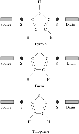
Figure 2: Schematic view of the three different molecular wires. The heterocyclic molecules (pyrrole, furan and thiophene) are attached to the electrodes, viz, source and the drain via thiol (S-H) groups.

and thiophene molecules respectively. These molecules are attached to the semi-infinite metallic electrodes by thiol (sulfur-hydrogen i.e., S-H bond) groups. In actual experimental set-up, the electrodes made from gold (Au) are used and the molecule coupled to the electrodes through thiol groups in the chemisorption technique where hydrogen (H) atoms remove and sulfur (S) atoms reside. To describe these heterocyclic molecules, we use the similar kind of non-interacting tight-binding Hamiltonian as given in Eq. (5).

All the essential features of this article are studied in the two distinct regimes. One is so-called the weak-coupling regime, defined by the condition $\tau_{\{S,D\}}<<t$. The other one is so-called the strong-coupling regime, denoted by the condition $\tau_{\{S,D\}}\sim t$. For these two limiting cases, we take the values of the different parameters as follows: $\tau_{S}=\tau_{D}=0.5$; $t=2.5$ (weak coupling) and $\tau_{S}=\tau_{D}=2$; $t=2.5$ (strong-coupling). Here we set the on-site energy $\epsilon_{0}=0$ (we can take any constant value of it instead of zero since it gives only the reference energy level) for the electrodes, and the hopping strength $v=4$ in the two semi-infinite metallic electrodes. For the sake of simplicity, here we set the Fermi energy $E_{F}=0$.

In Fig. 3, we plot the conductance $g$ as a function of the injecting electron energy $E$ for the three molecular wires, where the solid, dotted and dashed curves correspond to the results for the wires containing pyrrole, furan and thiophene molecules respectively. The results for the weak-coupling case are shown in Fig. 3(a), while Fig. 3(b) gives the results in the limit of strong molecular coupling. In the weak molecular coupling, the $g$-$E$ characteristics show sharp resonance peaks for some particular energy values, while they (resonance peaks) disappear for all other energies. These resonance peaks are associated with the energy eigenvalues of the individual molecules. Therefore we can say

Figure 3: Conductance $g$ as a function of the injecting electron energy $E$, where the solid, dotted and dashed curves correspond to the molecular wires with pyrrole, furan and thiophene molecules respectively. (a) weak-coupling limit and (b) strong-coupling limit.

that, the conductance spectrum manifests itself the electronic structure of the molecule. As expected, the maximum value of these conductance peaks goes to two i.e., the transmission probability ($T$) becomes unity since we get the relation $g=2T$ from the Landauer conductance formula, Eq. (1), with $e=h=1$ in our present formulation. From these results it is observed that the resonance peaks get shifted in the scale of the energy $E$ as we chemically change the heteroatoms in these heterocyclic molecules. Thus we can predict that the on/off state of the electron conduction across the molecule can be tuned by chemically modifying the heteroatoms, though in all these three molecular wires the molecular structures are the same. This provides an important finding in the study of molecular transport. In the strong molecule-to-electrodes coupling limit, these resonance peaks get substantial widths as presented in Fig. 3(b). Such increment of the resonance widths is due to the broadening of the molecular energy levels in the limit of strong molecular coupling, where the contribution comes from the imaginary parts of the self-energies $\Sigma_{S}$ and $\Sigma_{D}$,[38] as mentioned earlier in Section $2$. From the curves plotted in Figs. 3(a) and (b) it is observed that, the positions of the resonance peaks are independent of the molecule-to-electrodes coupling strength. Another significant feature observed from these curves is that, in the strong-coupling limit, the molecular bridge remains in the on-state condition i.e., electron passes through the molecule for a wide range of energies, while a fine tuning in the energy scale is necessary to get the on-state condition for that bridge in the limit of weak molecular coupling. This feature is quite significant in fabrication of efficient electronic circuits by using these molecules.

The scenario of the electron transfer through such molecular wires becomes much more clearly visible by describing the current-voltage characteristics, where the current passing across the molecule is computed from the integration procedure of the transmission function $T$ (see Eq. (9)). The variation of this transmission function looks similar to that of the conductance spectra (see Figs. 3(a) and (b)), differ only in magnitude by the factor $2$, since the relation $g=2T$ holds from the Landauer conductance formula as stated earlier. In Fig. 4, we display the current $I$ as a function of the applied bias voltage $V$ for the three molecular wires where the solid, dotted and dashed curves correspond to the same molecular systems as given in Fig. 3. The results for the weak-coupling limit are shown in Fig. 4(a), while Fig. 4(b) corresponds to the results in the limit of strong molecular coupling. In the limit of weak molecular coupling, the current-voltage characteristics give staircase-like behavior with sharp steps (Fig. 4(a)). This is due to the existence of the sharp resonance peaks in the conductance spectrum (Fig. 3(a)) since the current is evaluated from the integration procedure of the transmission function $T$. With the increase of the applied bias voltage, the electrochemical potentials on the electrodes are shifted gradually, and eventually cross one of the molecular energy levels. Accordingly, a current channel is opened up and the current-voltage curve produces a jump. The shape and height of these current steps depend on the width of the molecular resonances. With the increase of the molecular coupling strength, the current varies quite continuously with the bias voltage $V$, as illustrated in Fig. 4(b), and achieves much higher values. This can be understood by noting the areas under the curves in the conductance spectrum as plotted in Fig. 3(b) in the limit of strong molecular coupling.

Figure 4: Current $I$ as a function of the applied bias voltage $V$, where the solid, dotted and dashed curves correspond to the molecular wires with pyrrole, furan and thiophene molecules respectively. (a) weak-coupling limit and (b) strong-coupling limit.

From these results we predict that one can achieve much higher current amplitude in a molecular bridge system just by tuning the molecule-to-electrodes coupling strength, without changing any geometry of the bridge. The other most important feature appears from these current-voltage characteristics is that, the threshold bias voltage ($V_{th}$) of the electron conduction changes with the change of the heteroatoms in these heterocyclic molecules. Thus we can tune $V_{th}$ by chemically modifying the heteroatoms and this provides a key result in the study of molecular transport in these molecular wires.

4 Conclusion

In conclusion, we have explored the electron transport properties of the molecular wires made by the heterocyclic molecules (pyrrole, furan and thiophene), and observed that the transport properties are significantly influenced by (a) the heteroatoms in the molecules and (b) the molecule-to-electrodes coupling strength. Here we have used the simple tight-binding model to describe the molecular wires, and introduced a parametric approach to study the electron transport.

In the study of the $g$-$E$ characteristics we have noticed that the conductance shows very sharp resonance peaks (Fig. 3(a)) in the limit of weak molecular coupling associated with the molecular energy levels, while the widths of these resonances get enhanced substantially (Fig. 3(b)) in the strong molecular coupling limit. This is due to the broadening of the molecular energy levels in the limit of strong coupling, where the contribution comes from the imaginary parts of the two self energies $\Sigma_{S}$ and $\Sigma_{D}$.[38]

Next we have concentrated our study on the current-voltage characteristics from which the scenario of the electron transfer through the molecules can be understood much more clearly. The current changes its behavior from the staircase-like structure with sharp steps (Fig. 4(a)) to the continuous one (Fig. 4(b)) as the molecular coupling changes its strength from the weak regime to the strong one. From this study we have observed that the threshold bias voltage $V_{th}$ of the electron conduction can be tuned by chemically modifying the heteroatoms in these heterocyclic molecules.

Throughout our study we have used several realistic assumptions. More studies are expected to take the Schottky effect, comes from the charge transfer across the metal-molecule interfaces, the static Stark effect, which is taken into account for the modification of the electronic structure of the molecular bridge due to the applied bias voltage (essential especially for higher voltages). However all these effects can be included into our framework by a simple generalization of the given formalism described here. In this article we have also ignored the effects of all inelastic scattering processes, by assuming that the electrons move smoothly from the source to the drain subject only to elastic scattering within the junction, and electron-electron correlation to characterize the electronic transport through such heterocyclic molecules.

References

- [1] A. Nitzan, Annu. Rev. Phys. Chem. 52, 681 (2001).
- [2] A. Nitzan and M. A. Ratner, Science 300, 1384 (2003).
- [3] P. A. Orellana, M. L. Ladron de Guevara, M. Pacheco and A. Latge, Phys. Rev. B 68, 195321 (2003).
- [4] P. A. Orellana, F. Dominguez-Adame, I. Gomez and M. L. Ladron de Guevara, Phys. Rev. B 67, 085321 (2003).
- [5] S. M. Cronenwett, T. H. Oosterkamp and L. P. Kouwenhoven, Science 281, 5 (1998).
- [6] A. W. Holleitner, R. H. Blick, A. K. Huttel, K. Eber and J. P. Kotthaus, Science 297, 70 (2002).
- [7] A. Aviram and M. Ratner, Chem. Phys. Lett. 29, 277 (1974).
- [8] R. M. Metzger et al., J. Am. Chem. Soc. 119, 10455 (1997).
- [9] C. M. Fischer, M. Burghard, S. Roth and K. V. Klitzing, Appl. Phys. Lett. 66, 3331 (1995).
- [10] J. Chen, M. A. Reed, A. M. Rawlett and J. M. Tour, Science 286, 1550 (1999).
- [11] M. A. Reed, C. Zhou, C. J. Muller, T. P. Burgin and J. M. Tour, Science 278, 252 (1997).
- [12] T. Dadosh, Y. Gordin, R. Krahne, I. Khivrich, D. Mahalu, V. Frydman, J. Sperling, A. Yacoby and I. Bar-Joseph, Nature 436, 677 (2005).
- [13] R. Baer and D. Neuhauser, J. Am. Chem. Soc. 124, 4200 (2002).
- [14] D. Walter, D. Neuhauser and R. Baer, Chem. Phys. 299, 139 (2004).
- [15] K. Tagami, L. Wang and M. Tsukada, Nano Lett. 4, 209 (2004).
- [16] K. Walczak, Cent. Eur. J. Chem. 2, 524 (2004).
- [17] R. Baer and D. Neuhauser, Chem. Phys. 281, 353 (2002).
- [18] T. Kostyrko and B. R. BuÅa, Phys. Rev. B 67, 205331 (2003).
- [19] Y. M. Blanter and M. Buttiker, Phys. Rep. 336, 1 (2000).
- [20] K. Walczak, Phys. Stat. Sol. (b) 241, 2555 (2004).
- [21] M. Ernzerhof, M. Zhuang and P. Rocheleau, J. Chem. Phys. 123, 134704 (2005).
- [22] D. M. Newns, Phys. Rev. 178, 1123 (1969).
- [23] V. Mujica, M. Kemp and M. A. Ratner, J. Chem. Phys. 101, 6849 (1994).
- [24] V. Mujica, M. Kemp, A. E. Roitberg and M. A. Ratner, J. Chem. Phys. 104, 7296 (1996).
- [25] S. N. Yaliraki, A. E. Roitberg, C. Gonzalez, V. Mujica and M. A. Ratner, J. Chem. Phys. 111, 6997 (1999).
- [26] M. Di Ventra, S. T. Pantelides and N. D. Lang, Phys. Rev. Lett. 84, 979 (2000).
- [27] Y. Xue, S. Datta and M. A. Ratner, J. Chem. Phys. 115, 4292 (2001).
- [28] J. Taylor, H. Gou and J. Wang, Phys. Rev. B 63, 245407 (2001).
- [29] P. A. Derosa and J. M. Seminario, J. Phys. Chem. B 105, 471 (2001).
- [30] P. S. Damle, A. W. Ghosh and S. Datta, Phys. Rev. B 64, R201403 (2001).
- [31] M. Ernzerhof and M. Zhuang, Int. J. Quantum Chem. 101, 557 (2005).
- [32] M. Zhuang, P. Rocheleau and M. Ernzerhof, J. Chem. Phys. 122, 154705 (2005).
- [33] M. Zhuang and M. Ernzerhof, Phys. Rev. B 72, 073104 (2005).
- [34] W. W. Cheng, H. Chen, R. Note, H. Mizuseki and Y. Kawazoe, Physica E 25, 643 (2005).
- [35] W. W. Cheng, Y. X. Liao, H. Chen, R. Note, H. Mizuseki and Y. Kawazoe, Phys. Lett. A 326, 412 (2004).
- [36] M. P. Samanta, W. Tian, S. Datta, J. I. Henderson and C. P. Kubiak, Phys. Rev. B 53, R7626 (1996).
- [37] M. Hjort and S. Staftröm, Phys. Rev. B 62, 5245 (2000).
- [38] S. Datta, Electronic transport in mesoscopic systems, Cambridge University Press, Cambridge (1997).
- [39] M. B. Nardelli, Phys. Rev. B 60, 7828 (1999).
- [40] W. Tian, S. Datta, S. Hong, R. Reifenberger, J. I. Henderson and C. I. Kubiak, J. Chem. Phys. 109, 2874 (1998).