Triggered star formation
on the borders of the Galactic H ii region RCW 82

Abstract

Context. We are engaged in a multi-wavelength study of several Galactic H ii regions that exhibit signposts of triggered star formation on their borders, where the collect and collapse process could be at work.

Aims. When addressing the question of triggered star formation, it is critical to ensure the real association between the ionized gas and the neutral material observed nearby. In this paper we stress this point and present CO observations of the RCW 82 star forming region.

Methods. The velocity distribution of the molecular gas is combined with the study of young stellar objects (YSOs) detected in the direction of RCW 82. We discuss the YSO’s evolutionary status using near- and mid-IR data. The spatial and velocity distributions of the molecular gas are used to discuss the possible scenarios for the star formation around RCW 82.

Results. Several massive molecular condensations, together with star formation sites, are observed on the borders of RCW 82. The shapes of the three brightest condensations suggest that they were pre-existent, i.e. not formed through the collect and collapse process. A thin layer of molecular material is observed surrounding the ionized gas, adjacent to the ionization front. This results from the sweeping up of neutral material around the expanding region. Several Class I YSOs are detected in the direction of this layer.

Conclusions. The numerous YSOs observed towards the bright molecular condensations bordering (and velocity-associated with) the ionized gas reveal the intense star formation activity in RCW 82. But this region is probably too young to have triggered star formation via the collect and collapse process.

1 Introduction

The formation of massive stars can be triggered by H ii regions. Massive molecular condensations on the borders of Galactic H ii regions are the most likely sites for star formation and are consequently the most likely locations for observing the earliest stages of stellar births.

Several recent H ii region studies (Deharveng et al. deh03 (2003), Zavagno et al. zav06 (2006), Watson et al. Wat08 (2008), Cappa et al. cap08 (2008), Kirsanova et al. kir08 (2008)) have taken up the challenge to understand the triggered star formation processes, even if some points still remain not clear.

In the collect and collapse process, proposed by Elmegreen & Lada (elm77 (1977)), the expansion of the ionized region leads to the formation of a dense layer of material, collected between the ionization front (IF) and the shock front, during the supersonic expansion of the H ii region. This layer eventually becomes gravitationally unstable along its length and fragments, leading to the formation of massive condensations that are potential sites for subsequent star formation. In 2005, Deharveng et al. proposed a list of candidate Galactic H ii regions where the collect and collapse process may be the main triggering agent for the star formation observed on their borders. We have shown this process to be at work in a number of regions, among them Sh 104 (Deharveng et al. deh03 (2003)) and RCW 79 (Zavagno et al. zav06 (2006)). We have also shown that this process works in inhomogeneous turbulent clouds as in the cases of Sh2-212 (Deharveng et al. deh08 (2008)), Sh2-217 (Brand et al. in preparation) and Sh2-241 (Pomarès et al. in preparation).

The observations of an increasing number of sources show that the layer of collected neutral material is always present around the ionized gas and that various triggering processes are at work there.

Information about the distribution of associated molecular material is frequently lacking for these regions. We therefore carried out line observations of the molecular material, at velocities bracketing those of the surrounding ionized gas. Without such radial velocities we are never sure that a given condensation is indeed associated with the H ii region we are studying. The same is true of the YSOs that are observed in the direction of the region, with no more than a reasonable probability of being associated with it, based on the spatial distribution of these types of sources. We therefore carried out a series of molecular observations around H ii regions using the Mopra radio-telescope. The first results are presented here for RCW 82, along with a discussion of the YSO population using new near-IR, Spitzer-GLIMPSE and MIPSGAL mid-IR data.

This paper is organized as follows: Sect. 2 presents the Galactic H ii region RCW 82. New observations towards this region are presented in Sect. 3. Results are given in Sect. 4. Sect. 5 presents a general discussion about the morphology of the region and the star formation processes at work there. Conclusions are given in Sect. 6.

2 Presentation of RCW 82

RCW 82 (Rodgers et al. rod60 (1960)) is an optical H ii region centred at $\alpha_{2000}$=13^h 59^m 30^s, $\delta_{2000}$=$-$61^∘ 23^′ 30^′′ ($l$=310$.\!\!^{\circ}$99, $b$=0$.\!\!^{\circ}$41). Its diameter is $\sim$6^′ ($\sim$6 pc for a distance of 3.4 kpc).

RCW 82 is a thermal radio-continuum source (Whiteoak et al. whi94 (1994)). Its radio flux density is very badly constrained from the literature: $S_{\rm{5\leavevmode\nobreak\ GHz}}=0.73$ Jy (Haynes et al. hay79 (1979)), $S_{\rm{5\leavevmode\nobreak\ GHz}}=4.6$ Jy (Caswell & Haynes cas87 (1987); resolution 4$.\mkern-4.0mu^{\prime}$2), $S_{\rm{4.85\leavevmode\nobreak\ GHz}}=1.302$ Jy (Kuchar et al. kuc97 (1997)), $S_{\rm{843\leavevmode\nobreak\ MHz}}=1.5$ Jy (Cohen et al. coh07 (2007); resolution 43^′′).

Fig. 1 shows the emission from the ionized gas. The H$\alpha$ emission (gray scale image) is from the SuperCOSMOS survey (Parker et al. par05 (2005)). The contours are for the SUMSS survey at 843 MHz (FWHM $43\hbox{${}^{\prime\prime}$}\times 43\hbox{${}^{\prime\prime}$}\cos(\delta)$; Bock, Large, & Sadler boc99 (1999)). A radio point source is present in the direction of the ionized gas, at $\alpha_{2000}$=13^h 59^m 10${}^{\rm s}.72$, $\delta_{2000}$=$-$61^∘ 23^′ 00^′′. At 843 MHz the emission is strongly weighted by non-thermal emission, if any is present. It is not clear if this point source is thermal, or if it is a non-thermal background source, possibly a galaxy (its flux density at 843 MHz is $\sim 70$ mJy, M. Cohen, private communication).

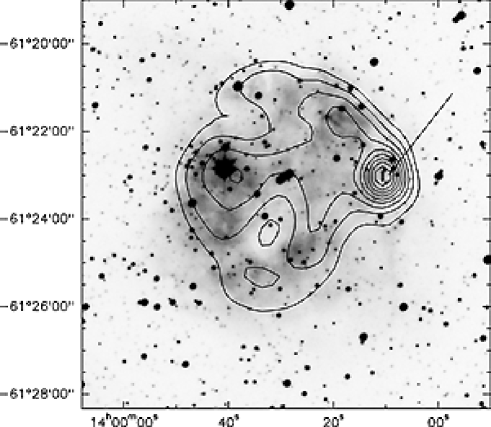
Figure 1: SuperCOSMOS image of RCW 82, showing the H$\alpha$ emission of the ionized gas. The contours are for the SUMSS survey at 843 MHz (FWHM $43\hbox{${}^{\prime\prime}$}\times 43\hbox{${}^{\prime\prime}$}\cos(\delta)$). The first contour is at 0.02 Jy/beam, and the step is 0.01 Jy/beam. The arrow points to the radio-continuum point source discussed in the text.

2.1 RCW 82 in the infrared

RCW 82 was observed by the infrared satellite MSX (Mid-course Space eXperiment), from 8.3 $\mu$m to 21.3 $\mu$m (Price et al. pri01 (2001)). Deharveng et al. (deh05 (2005)) present a colour composite image of RCW 82 (their Fig. 1). At 8.3 $\mu$m, RCW 82 appears as an empty bubble. The MSX band at 8.3 $\mu$m contains, superimposed on a continuum, emission bands attributed to large molecules such as polycyclic aromatic hydrocarbons (PAHs; Léger & Puget leg84 (1984)). These molecules are destroyed inside the ionized gas, but are excited in the photodissociation region (PDR) by the radiation leaking from the H ii region. On the other hand, part of the 21.3 $\mu$m emission comes from small grains within the ionized gas of the bubble. Small grains can survive in strong UV fields, while large molecules cannot (Crété et al. cre99 (1999), Peeters et al. pee02 (2002)). RCW 82 (S 137 in Churchwell et al.’s catalogue, chu06 (2006)) is one of the many bubbles detected by the Spitzer infrared satellite in the Galactic plane. Fig. 2 is a colour composite image of RCW 82, showing the H$\alpha$ emission of the ionized gas (from the SuperCOSMOS survey) in blue, the emission at 3.6 $\mu$m in green (mainly stellar emission), from the Spitzer-GLIMPSE survey (Benjamin et al. ben03 (2003)), and the PAH emission at 8.0 $\mu$m in red (Spitzer-GLIMPSE survey). This confirms, with higher spatial resolution and sensitivity, the view given by MSX. The PAH emission comes from the hot photo-dissociation zone surrounding the ionized region. This zone is extended, but the brightest emission comes from a thin layer adjacent to the ionization front.

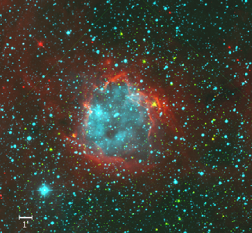
Figure 2: Colour composite image of RCW 82. Spitzer-IRAC 8.0 $\mu$m (red) and 3.6 $\mu$m (green) images from the Spitzer-GLIMPSE survey have been combined with the H$\alpha$ (blue) image from the SuperCOSMOS survey. A PAH emission layer, emitted by the hot photo-dissociation region, surrounds the ionized region. The field size is 20$.\mkern-4.0mu^{\prime}$0 (E-W) $\times$ 18$.\mkern-4.0mu^{\prime}$5 (N-S). North is up and east is left.

The Spitzer-MIPSGAL emission at 24 $\mu$m (Carey et al. car05 (2005)) is dominated by the continuum emission of small grains, located either in the extended ionized region and its PDR, or in the envelopes or disks associated with YSOs. This is illustrated by Fig. 3, a colour composite image of RCW 82, showing the stellar emission at 4.5 $\mu$m (in blue), the PAH emission at 8.0 $\mu$m (in green), and the 24 $\mu$m emission of the small grains (in red). YSOs and red giants are strong emitters at 24 $\mu$m. Two bright YSOs (indicated by arrows on Fig. 3) are diametrically opposite each other on the border of RCW 82; they will be discussed in Sect. 5.2.2. We also see the extended emission of the small grains located inside the H ii region. However, their distribution differs from that of the ionized gas: i) they are located in the very central zone; this may be due to a higher temperature of the grains close to the central exciting star(s); ii) their emission is not enhanced in the direction of the radio-continuum point source (arrow in Fig. 1); this suggests that this radio point source is an unrelated non-thermal background source.

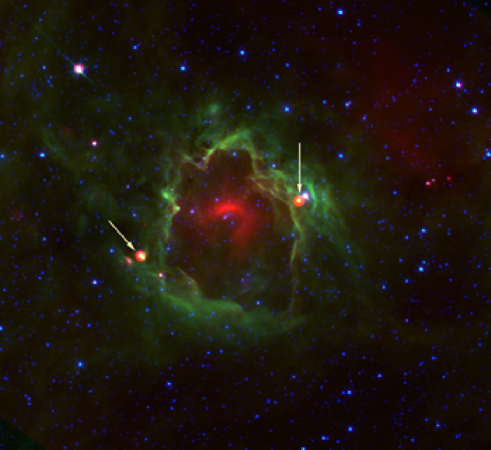
Figure 3: Colour composite image of RCW 82. Red is the emission of small grains at 24 $\mu$m, from the Spitzer-MIPSGAL survey, green is the PAH emission at 8.0 $\mu$m, and blue the 4.5 $\mu$m emission, from the Spitzer-GLIMPSE survey. North is up, east is left. The arrows point to the two main star formation sites discussed in Sect 5.2.2. The east and west arrows point to the cluster and to the YSO $\#$106, respectively.

RCW 82 is situated on the southeastern border of a $\sim 27\hbox{${}^{\prime}$}$ diameter shell. Fig. 4 shows a colour composite image of this shell, with 8.0 $\mu$m emission in turquoise and 24 $\mu$m emission in red. Diffuse radio emission at 843 MHz is detected by the SUMSS in the direction of the shell interior, suggesting the presence of ionized gas within the shell. Most probably the shell surrounds an H ii region, and the 24 $\mu$m emission arise from small dust grains surviving with the ionized gas, as it is the case for RCW 82. We also see several very luminous red sources in the direction of the shell. They are associated with dark filaments seen in absorption at 8 $\mu$m, probably tracing very dense material. Fig. 4 suggests that the formation of RCW 82 could have been triggered by the expansion of the large shell. However, we do not know the shell’s distance, and whether it is really associated with RCW 82. This shell is faint and is not detected on the IRAS survey. We searched the H i (continuum and line) SGPS data (McClure-Griffiths et al. mcc01 (2001)) to identify this structure. Continuum emission at 21 cm confirms that ionized gas is observed towards the interior of the shell, as well as in RCW 82. However, 21 cm line emission is observed everywhere and the large shell is not clearly outlined. Large scale, higher resolution data are needed to address the association of RCW 82 with this large bubble.

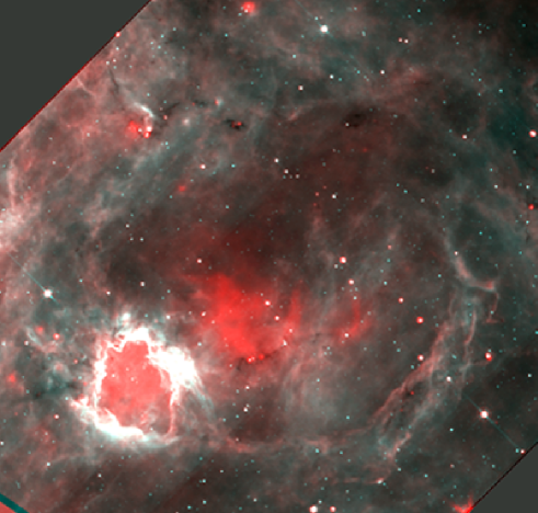
Figure 4: Large scale composite colour image of RCW 82 and its surroundings. The 8 $\mu$m emission from Spitzer-GLIMPSE appears in turquoise and the 24 $\mu$m emission from Spitzer-MIPSGAL in red. North is up, east is left.

2.2 The exciting star(s) of RCW 82

No exciting star of RCW 82 was identified in the literature. Here we offer indirect evidence suggesting the possible location and properties of the exciting star(s).

The first piece of information is given by the radio continuum emission of RCW 82. We used equation (1) of Simpson & Rubin (sim90 (1990)) to estimate the number of ionizing Lyman continuum photons $N_{\rm{Lyc}}$ emitted by the exciting star(s) from the radio-continuum flux density; Using the radio flux $S_{5\leavevmode\nobreak\ \rm{GHz}}=4.6$ Jy (Caswell & Haynes cas87 (1987)), supposing an electron temperature $T_{\rm{e}}=10000$ K and a distance of 3.4 kpc, we obtain $\log(N_{\rm{Lyc}}$)$\sim$48.7 photons per second. According to the calibration of O stars by Martins, Schaerer & Hillier (mar05 (2005)), this corresponds to a spectral type $\sim$O7V (assuming a single main-sequence exciting star).

The second indication concerns the location of the exciting star(s). Four stars lying near the upper centre of RCW 82 are candidates. Our selection is based on the following reasons:

$\bullet$ The H ii region is almost circular. Hence the exciting star(s) are expected near its centre.

$\bullet$ The IF shows some structures (like “pillars” or “fingers”) protruding inside the ionized region (Fig. 5). Such structures, shaped by the UV radiation field, usually point towards the exciting stars (Osterbrock ost57 (1957)). Here, they point to the four central stars.

$\bullet$ Another argument is the presence of a hole in the 24 $\mu$m emission in the centre of RCW 82, seen in the direction of these four stars, and the annular shape of the dust emission delimiting its border, clearly seen in Fig. 3. This feature is observed in several H ii regions such as RCW 120 (Zavagno et al. zav07 (2007)) and N 49 (Watson et al. Wat08 (2008)) around the exciting stars.

Fig. 5 shows these stars, labelled from e1 to e4, at different wavelengths, from the near-IR to 24 $\mu$m. These stars have similar $K$-band fluxes, but e2 and e3 decrease in brightness with increasing wavelength, while e4 is brightest in $K$. Also e1 is brighter than e2 and e3 in the mid-IR; it is the only star detected at 24 $\mu$m.

We used the 2MASS and Spitzer-GLIMPSE magnitudes to determine the nature of these four stars, and especially whether they could be O stars. The 2MASS $J-H$ vs. $H-K$ diagram (Fig. 15) shows that e4 is probably a giant, that e1 presents a small near-IR excess, and that e2 and e3 are probably main sequence stars. The $J$ vs. $J-K$ diagram (not shown here) confirms that e4 is a giant, and that stars e2 and e3 are O type stars – possibly O7.5V and O6.5V stars with a visual extinction $\sim$ 4.2 mag and 4.7 mag, respectively. In the Spitzer $[3.6]-[4.5]$ vs. $[5.8]-[8.0]$ colour-colour diagram (Fig 13) star e1 again shows an infrared excess (it appears close to the Class II YSO area of the diagram), whereas stars e2, e3 and e4 are situated in the group of main-sequence and giant stars. Thus we propose that stars e2 and e3 participate in the excitation of the H ii region; the part played by star e1, possibly still accreting material through a disk, is uncertain. Star e4, a giant, is possibly unassociated with RCW 82.

According to Martins, Schaerer & Hillier (mar05 (2005)) the ionizing flux of an O7.5V plus an 06.5V stars is $\sim 9\times 10^{48}\leavevmode\nobreak\ s^{-1}$, thus slightly larger than necessary to account for the observed radio flux density of RCW 82. Some of these ionizing photons are possibly used to heat the dust emitting at 24 $\mu$m in the ionized gas.

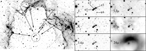
Figure 5: The four candidate exciting stars, e1, e2, e3, and e4. Left: unsharp masked image at 5.8 $\mu$m (from Spitzer-GLIMPSE) showing bright rims and “fingers” pointing to the candidate exciting stars. Right: the four central stars at various wavelengths.

3 New observations and data reduction

3.1 Molecular Observations

We used the 22-m Mopra single-dish radio telescope to study the distribution of the molecular material associated with RCW 82. This antenna has a full width at half maximum (FWHM) of 33^′′$\pm$2^′′and a main beam efficiency of 0.42 at a frequency of 115 GHz (Ladd et al. lad05 (2005)). Observations were undertaken in on-the-fly (OTF) mapping mode using the Mopra-MOPS digital filterbank (MOPS-DFB) spectrometre in July and August 2007. The MOPS-DFB has a bandwidth of 8 GHz, and can operate in either broadband or zoom mode (see Jones et al. jon08 (2008) for more information). We used the zoom mode of the MOPS Spectrometre, with 12 ’zoom’ windows of width 137 MHz, with 4096 channels each, giving a velocity resolution of 0.09 km s^-1. The pointing was done using nearby SiO masers, with the pointing being generally better than 10^′′. Individual maps of 5^′ $\times$ 5^′ were combined to cover a field of 12$.\mkern-4.0mu^{\prime}$5 $\times$ 12$.\mkern-4.0mu^{\prime}$5 centred on RCW 82. The OTF maps were made in a similar way to that described in Bains et al. (bai06 (2006)). Position switching was used for calibration, with the offset reference position l=310.6, b=+1.5 being observed after each row of an OTF map. The scan rate was 2^′′ per second, and the spectra were read out with 2 seconds of integration time. The scan lines were separated by about 10^′′. Each map took 85 mins to complete, which included 72 mins of on-source time. Each 5^′ $\times$ 5^′ region was mapped twice, once scanning in right ascension, and once scanning in declination. Several lines were observed simultaneously; the lines detected were ¹²CO(1-0) (115.271 GHz), ¹³CO(1-0) (110.201 GHz) and C¹⁸O(1-0) (109.782 GHz).

Data reduction was done with the ATNF GRIDZILLA and LIVEDATA packages (http://www.atnf.csiro.au/computing/software/). Using LIVEDATA, we fitted a linear baseline, computed using emission-free channels, and subtracted it from each 5$\hbox{${}^{\prime}$}\leavevmode\nobreak\ \times\leavevmode\nobreak\ 5\hbox{${}^{\prime}$}$ map. We then used GRIDZILLA with a 0$.\mkern-4.0mu^{\prime}$25 FWHM Gaussian smoothing with a pixel size of 0$.\mkern-4.0mu^{\prime}$2 to grid the spectra into datacubes. In this way we obtained data cubes covering the velocity range $-100$ to $100$ km s^-1 for each spectral line.

3.2 Near-IR observations

NTT-SofI observations were obtained at La Silla (Chile) on 15 February 2003, in the $J$ (1.247 $\mu$m), $H$ (1.653 $\mu$m) and $K_{\rm{S}}$ (2.162 $\mu$m) bands.

Two fields of $\sim$ 2.6^′ $\times$ 2.6^′ were observed. Field 1 is centred on the MSX point source G331.0341+00.3791 centred at $\alpha_{2000}$=13^h 59^m 57$.\!\!^{\rm s}$4, $\delta_{2000}$=$-$61^∘ 24^′ 32$.\!\!^{\prime\prime}$9 (see Fig 3). The position of this MSX source is indicated in the paper Deharveng et al. (deh05 (2005)), where the numbers of the sources in their Fig. 18 are reversed by mistake. Field 2 is centred at $\alpha_{2000}$=13^h 59^m 45$.\!\!^{\rm s}$6, $\delta_{2000}$=$-$61^∘ 22^′ 54$.\!\!^{\prime\prime}$5, on the ionization front.

The images were reduced with the procedure described by Zavagno et al. (zav06 (2006)) for the RCW 79 H ii region. For field 1, the total exposure times are 250 s, 36 s and 12 s respectively in $J$, $H$ and $K_{\rm{S}}$. For field 2, they were 100 s in $J$, 60 s in $H$ and 24 s in $K_{\rm{S}}$. The photometry was performed using DAOPHOT (Stetson ste87 (1987)), also as described in Zavagno et al. (zav06 (2006)).

4 Results

4.1 H$\alpha$ velocity field

Large scale H$\alpha$ emission from the ionized gas around RCW 82 was reported by Russeil et al. (rus98 (1998)). They showed that in addition to the local diffuse emission, widely distributed diffuse emission is detected at velocities around $-$31 km s^-1 and $-$50 km s^-1. Using the stellar distance of the OB stars and clusters in the “313^∘ zone” one can place the $-$31 km s^-1 layer at 1.5 $\pm$ 0.3 kpc and the $-$50 km s^-1 layer at 3.4 $\pm$ 0.9 kpc (Russeil et al. rus98 (1998)). With an H$\alpha$ systemic velocity of $-$50 km s^-1 (obtained from the profile integrated over the total H ii region) RCW 82 clearly belongs to the more distant layer. From these same data we can carry out a detailed study of the internal kinematics of RCW 82 (Fig. 6). The FWHM line width of the fitted gaussian components has a typical value, between 23 and 25 km s^-1, except at three positions where it is less than 20 km s^-1. These positions are located on the border of the ionized region.

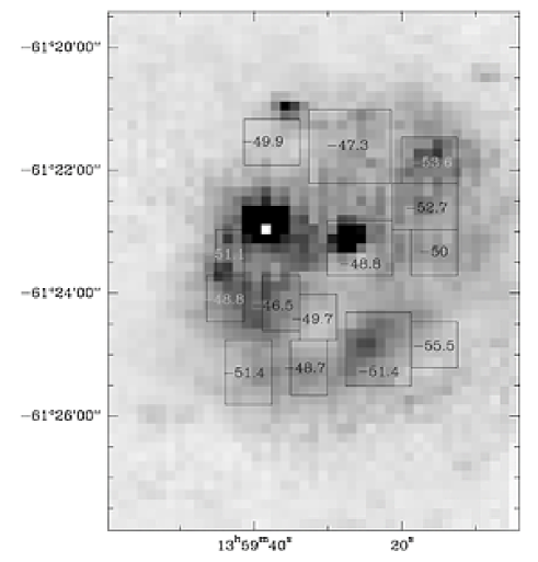
Figure 6: H$\alpha$ Velocity field of RCW 82. The velocities obtained over the selected areas are shown. The values in white correspond to the regions where small line width is observed.

4.2 The molecular materiel

4.2.1 Spatial distribution of the molecular materiel

We used the ¹²CO, ¹³CO and C¹⁸O datacubes to study the dynamics of the molecular material detected in the direction of RCW 82 and to determine some physical properties of the observed condensations. The first step is to isolate the molecular components along the line of sight that are associated with the H ii region. Fig. 7 shows the velocity profile of the ¹²CO emission, integrated over the whole field, between $-70$ and $+30$ km s^-1 (no CO emission is seen outside this velocity range), obtained using MIRIAD (Sault et al. sau95 (1995)). We detect at least five velocity components along the line of sight. The brightest ones are centred at $-48$ and $-55$ km s^-1. Two intermediate ones are seen at about $-35$ and $-39$ km s^-1. Another component is detected a a positive velocity, $+16$ km s^-1.

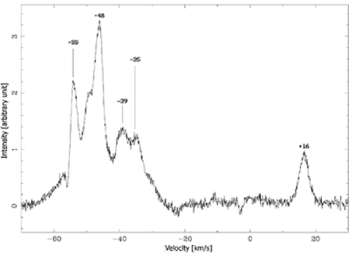
Figure 7: Integrated emission of ¹²CO (linear arbitrary unit) on the RCW 82 line of sight. Velocities are indicated for the different emission components mentioned in the text.

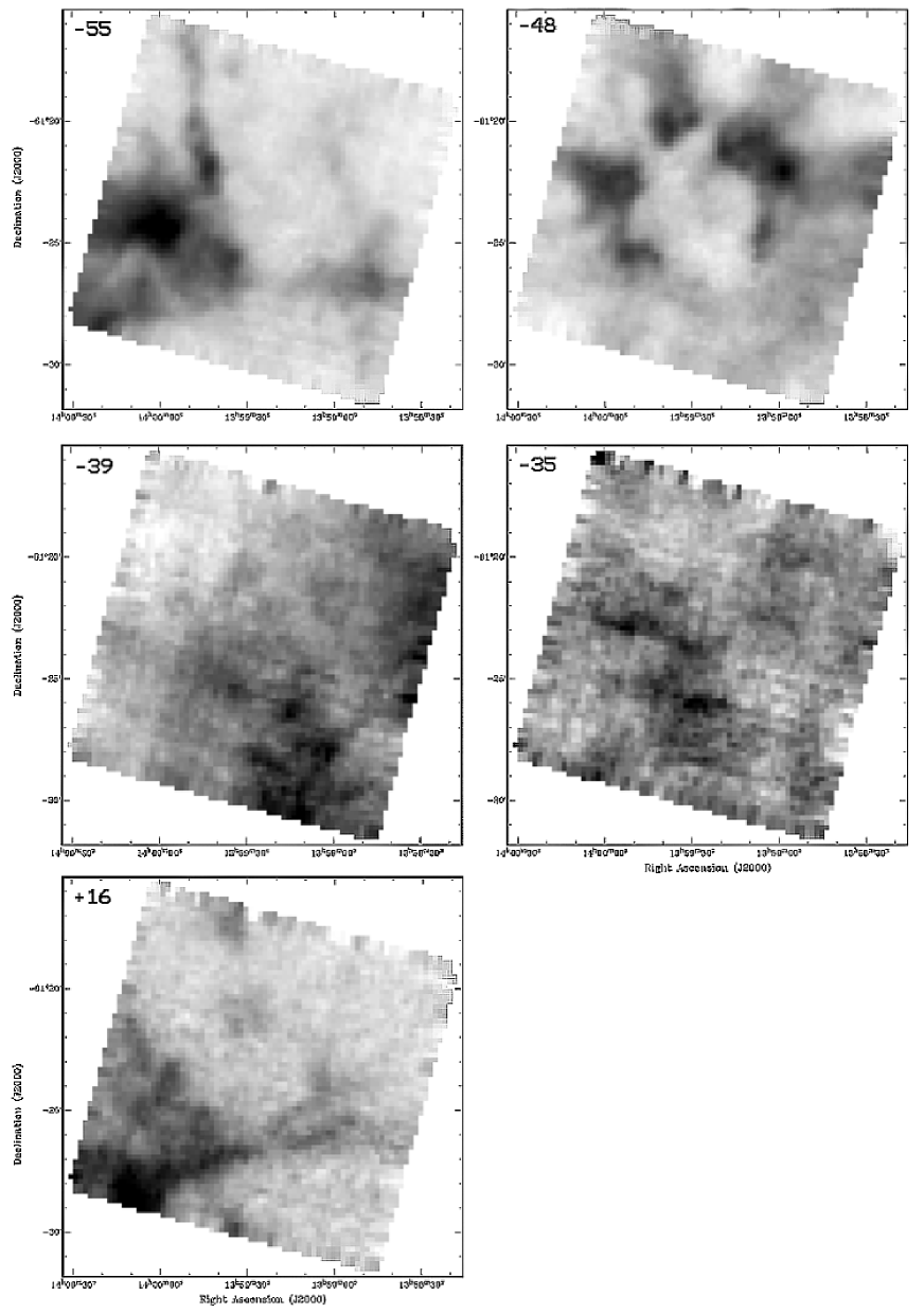
Figure 8: The different components seen in ¹²CO on the line of sight toward RCW 82. The velocity ranges for each integration are respectively $-57.06$ to $-52.07$, $-52.07$ to $-41.99$, $-41.99$ to $-36.35$, $-36.35$ to $-23.06$ and $+10.06$ to $+22.07$ km s^-1. The central velocity is given at the top left of each panel, in km s^-1. The gray scale is in units of K km s^-1, with darker shades indicating higher values.

We isolated these 5 molecular components. Fig. 8 shows the morphology of the corresponding emitting regions.

$\bullet$ The $-55$ km s^-1 component is seen as a strong emission, mainly on the east side of the H ii region and partly on its southwest side. At this velocity, the molecular material may be interacting with RCW 82, since H$\alpha$ emission from the H ii region is seen at a similar velocity (Fig. 6). The V-shape filamentary molecular emission associated with the $-55$ km s^-1 component (see Fig. 8) follows the 8 $\mu$m emission associated with the large bubble (Fig. 4). This association could indicate dynamical interactions between this large bubble and RCW 82. Unfortunately our spatial coverage of Mopra observations is not sufficient to make this association more clear. The dense emission peak (see Fig. 8 and Fig. 20) coincides with a dark structure seen at 8 $\mu$m (Fig. 4).

$\bullet$ The molecular component centred at $-48$ km s^-1 almost completely surrounds the ionized region. It consists of a thin layer (about 50^′′ thick (beam-corrected) or 0.8 pc at a distance of 3.4 kpc) together with a number of large clumps. Some of these clumps have cometary tails. H$\alpha$ emission from RCW 82 is observed at a velocity of about $-50$ km s^-1 (Russeil et al. rus98 (1998)). Based on velocity and morphological arguments we associate the molecular component centred at about $-48$ km s^-1 with the H ii region. This point is well illustrated by Fig. 9 which shows the excellent correspondence between molecular emission integrated between $-42$ and $-52$ km s^-1 and the border of the H ii region (outlined by the 24 $\mu$m emission of the PDR).

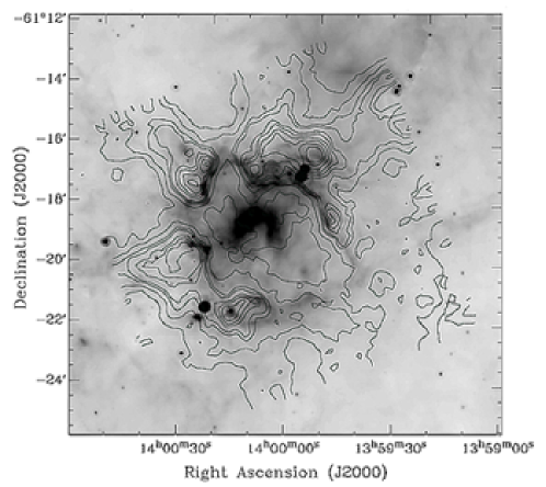
Figure 9: Isocontours of the ¹²CO emission integrated between $-42$ and $-52$ km.s^-1 superimposed on the 24 $\mu$m emission of RCW 82 taken from the Spitzer-MIPSGAL survey.

$\bullet$ The two components centred at $-39$ and $-35$ km s^-1 are probably not associated to RCW 82. They mainly consist of diffuse emission that extends throughout the field. The $-39$ km s^-1 component shows two emission peaks in the middle of the field, in the direction of the interior of RCW 82 (Fig. 8). The $-35$ km s^-1 component shows four emission peaks. Three of them are observed in the direction of the interior of RCW 82. They do not correspond to any absorption structures observed for example in the optical; thus these condensations are probably situated behind RCW 82 (the kinematic distances associated with the $-35$ km s^-1 velocity are 8.54 and 2.60 kpc, using the galactic rotation curve of Brand & Blitz bra93 (1993)).

$\bullet$ The $+16$ km s^-1 component lies very far from the H ii region, at 12.6 kpc from the sun, according to the Galactic rotation curve of Brand & Blitz (bra93 (1993)).

To conclude, based on velocity and morphology arguments, we consider in the following that the structure in the velocity range $-42$ to $-52$ km s^-1 is associated with RCW 82, but we bear in mind that the molecular emission centred at $-55$ km s^-1 could also be in interaction with RCW 82, even if it seems to be morphologically unrelated.

Fig. 10 and 11 show ¹²CO and ¹³CO emission associated with RCW 82, integrated over small velocity ranges of $\sim$1.6 km s^-1 wide, from $-51.81$ to $-41.38$ km s^-1. The emission peaks around $-48$ km s^-1. This velocity is slightly different from the velocity of the ionized gas: $-50$ km s^-1 from the H$\alpha$ line (Russeil et al. rus98 (1998)) or $-51$ km s^-1 from the H 109$\alpha$ line (Caswell & Haynes cas87 (1987)).

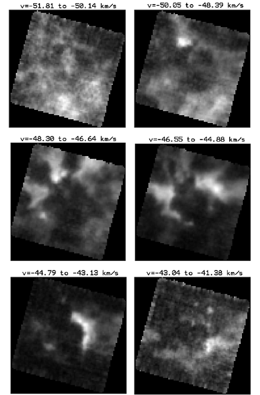
Figure 10: Integrated ¹²CO emission in the direction of RCW 82. Velocity ranges are indicated on the top of each image.

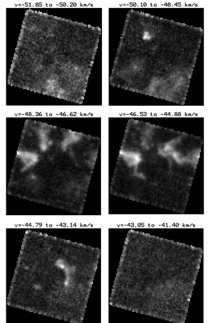
Figure 11: Integrated ¹³CO emission in the direction of RCW 82.

We now briefly describe the molecular material associated with RCW 82 shown in figures 10 and 11. To make this description clearer, we use the numbering of the molecular structures shown in Fig. 12.

From $-51.85$ to $-50.14$ km s^-1 two clumps of ¹²CO emission are seen southeast and southwest of the H ii region; these two clumps are also seen in ¹³CO. Some faint ¹²CO emission is observed towards the centre of the ionized region but is not detected in ¹³CO.

From $-50.05$ to $-48.40$ km s^-1 the southern emission is still present, and the clump $\#$1a appears north of the H ii region. Also, clump $\#$3 is seen on the southeast border.

From $-48.30$ to $-46.63$ km s^-1 the emission is seen mainly on the northeastern part of the ionized region. Clump $\#$3 observed on the east border is brighter. The same is observed for structure $\#$1 which now shows a cometary tail and a secondary peak on the west (structure 1b). Structures $\#$2, $\#$4 and $\#$5 appear on either side of the ionized region (north and northeast of the H ii region). They show cometary tails extending perpendicular to the ionization front. These structures are separated by holes in the CO emission. Fig. 18 shows ionized gas (H$\alpha$ emission) passing between structures $\#$1 and $\#$2. The ‘leakage’ of FUV radiation into these gaps might help to form the shapes of the molecular condensations.

From $-46.55$ to $-43.13$ km s^-1: Structure $\#$1 disappears, but structures $\#$5 and $\#$6 become brighter. On this same side we also see a thin layer of material adjacent to the ionization front (structure $\#$7). This is probably the shell of collected material compressed between the ionization front and the shock front expanding with the H ii region, as predicted by the collect and collapse theory (Elmegreen & Lada elm77 (1977)). The western part of this layer is not exactly at the same velocity but begins to appear. On the western counterpart the fragment is now larger and denser and seems to be elongated at both its extremities. This strange shape is compatible with the idea that some structures are due to pre-existing clouds.

From $-44.79$ to $-43.14$ km s^-1 almost all the clumps have disappeared. In this velocity range we see the western part of the collected material (structure $\#$7) which seems to be about 50^′′ in size (beam corrected) on the ¹²CO emission map (Fig. 10). The ¹³CO emission (Fig. 11) shows that the layer seems to be fragmented. The collect and collapse process predicts gravitational instabilities in the collected layer. The observation of cores agrees with this point, showing that the fragmentation phase has occurred for RCW 82. This point is discussed in section 5.3.

Only the brightest condensations are detected by our C¹⁸O observations (not shown here), mainly the clumps situated north of RCW 82 (structures $\#$1a, $\#$2, $\#$5 and $\#$6). This confirms that the surrounding molecular material is probably denser in the north than in the south.

4.2.2 H₂ column density

We estimated the $N$(H₂) column density from the ¹²CO and ¹³CO observations; the C¹⁸O emission is too weak over the field to be used, except in some specific locations. An upper limit to the total column density of ¹³CO can be derived by making the assumption that all rotational levels are thermalized with the same excitation temperature $T_{\rm{K}}=T_{\rm{ex}}$ (LTE assumption). The map of the excitation temperature is obtained from the peak brightness temperature of ¹²CO(1-0), assumed to be optically thick, and corrected for the cosmic background emission, via

$$T_{\rm{ex}}=\frac{5.532}{\ln(\frac{5.532}{T_{B}^{*}+0.840}+1)}.$$ (1)

The map we obtain shows temperatures up to 37 K.

The total column density map of ¹³CO is obtained assuming that the ¹³CO(1-0) emission is optically thin, so that

$$N_{\rm{Tot}}(^{13}\rm{CO})=U_{T_{\rm{ex}}}\frac{8\pi}{c^{3}}\frac{\nu_{0}^{2}}{g_{u}A_{ul}}e^{\frac{E_{l}}{kT_{\rm{ex}}}}\frac{k}{h}\int_{-\infty}^{+\infty}T_{\rm{mb}}\,d\rm{v}$$ (2)

where $U_{T_{\rm{ex}}}=0.7597\times T_{\rm{ex}}$ is the partition function for ¹³CO (Müller et al. mul05 (2005)).

Then, assuming LTE we use the conversion factor H₂/¹³CO=6$\times$10⁵ (obtained from the “canonical value” ¹²CO/H₂=10^-4 (van Dishoeck et al. vanDi92 (1992)) and the isotopic abundance ¹²CO/¹³CO=60), we can calculate the H₂ column density:

$$N(\rm{H_{2}})=6\times 10^{5}\leavevmode\nobreak\ N(^{13}\rm{CO})$$ (3)

The column density map of H₂ obtained using ¹³CO data via equations 2 and 3 is presented in Fig. 12. It shows several condensations as well as structures resulting from the accumulated material around the ionized region during its expansion.

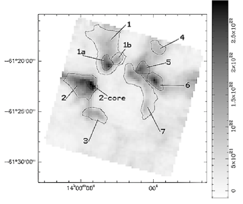
Figure 12: Map of H₂ column density obtained from the ¹³CO data, assuming that the ¹³CO emission is optically thin. The structures discussed in the text are identified. The solid contours are the limits chosen to define the structures presented in Table 1.

It is important to note that the coefficients used for the conversion from $N$(¹²CO) and $N$(¹³CO) to $N$(H₂) are quite uncertain, and therefore the masses of the condensations are uncertain as well.

4.2.3 Molecular condensations

Table 1: Mass of the molecular structures observed around RCW 82.

Structure	$\alpha_{2000}$	$\delta_{2000}$	velocity range	N(H2) peak	N(H2) level	mass
			(km s-1)	(cm-2)	(cm-2)	($M_{\odot}$)
1	13h 59m 36.86s	-61∘ 19′ 14.5′′	$-50.10$ to $-45.80$		2.5 $\times$ 1021	2300
1a	13h 59m 37.08s	-61∘ 20′ 18.97′′	$-50.10$ to $-45.80$	2.4 $\times$ 1022	1.3 $\times$ 1022	620
1b	13h 59m 30.40s	-61∘ 19′ 55.00′′	$-48.45$ to $-45.98$	1.7 $\times$ 1022	3.0 $\times$ 1021	187
2	13h 59m 57.96s	-61∘ 22′ 17.3′′	$-48.09$ to $-44.79$		9.0 $\times$ 1021	2560
2-core	13h 59m 52.12s	-61∘ 22′ 30.84′′	$-48.09$ to $-44.79$	2.7 $\times$ 1022	2.3 $\times$ 1022	355
3	13h 59m 47.14s	-61∘ 25′ 18.90′′	$-46.35$ to $-44.51$	7.9 $\times$ 1021	1.5 $\times$ 1021	255
4	13h 58m 57.15s	-61∘ 18′ 45.22′′	$-48.09$ to $-46.35$	8.7 $\times$ 1021	6.5 $\times$ 1021	283
5	13h 59m 10.39s	-61∘ 20′ 30.95′′	$-46.90$ to $-45.34$	1.5 $\times$ 1022	9.0 $\times$ 1021	386
6	13h 58m 58.78s	-61∘ 21′ 56.65′′	$-46.71$ to $-44.79$	2.1 $\times$ 1022	9.0 $\times$ 1021	626
7	13h 59m 5.36s	-61∘ 22′ 54.91′′	$-46.35$ to $-43.14$	1.4 $\times$ 1022	2.0 $\times$ 1021	1100
8	14h 00m 01.75s	-61∘ 24′ 01.1′′	$-52.79$ to $-56.61$		1.5 $\times$ 1022	1500
8-core	13h 59m 59.61s	-61∘ 24′ 19.1′′	$-52.79$ to $-56.61$	3.24 $\times$ 1022	2.0 $\times$ 1022	780

We identified several molecular structures around RCW 82 (see Figs. 12 and 20). These structures are clumps and fragments, selected by eye in the ¹²CO and ¹³CO data cubes. Each structure is observed over a given velocity range. Maps of the column density were obtained for each of these velocity ranges. The mass of the structures is then deduced from the column density integrated over the spatial extent of the structures. The results are given in Table 1. The first column gives the identification of the structure, as in Fig. 12 and 20. Columns 2 and 3 are the coordinates of the approximate centr of the structure. Column 4 is the velocity range over which the structure is seen, and column 5 gives the column density at the emission peak. Column 6 is the N(H₂) value used to define the integration boundary and derive the mass, and column 7 gives the resulting masses. The masses given in Table 1 have been derived from N(¹³CO).

We compared these masses to those obtained using the ¹²CO emission alone, via eq. 17 of Rosolowsky et al. (ros06 (2006)). This formula uses a CO-to-H₂ conversion factor $X_{\rm{CO}}$=2$\times$10²⁰ cm^-2 (K km s^-1)^-1 and takes into account the presence of helium in the mass calculation. The derived masses differ by up to 50 percent from the values given in Table 1. This discrepancy can be explained by the uncertainty on the conversion factors we used, and by the fact that the densest clumps are probably optically thick in ¹²CO (thus the ¹²CO masses are underestimated). This argument is confirmed by the N(H₂) column density map we obtain via the ¹²CO (not shown here), which shows lower column densities in the direction of the densest part of the condensations than those obtained with the ¹³CO.

Massive molecular structures are thus observed all around RCW 82. They contain enough material to form massive objects, stars or clusters. A number of these structures are adjacent to the ionization front ($\#$ 1a, $\#$ 1b, $\#$ 2-core). It is not possible to know if they were pre-existent clumps suddenly submitted to the pressure of the ionized gas, or if they are fragments resulting from the gravitational collapse of the collected shell. Structures $\#$ 3 and $\#$ 7 are clearly parts of this collected shell. Figs. 10 and 11 show that substructures are present in the collected layer.

4.3 A search for YSOs towards RCW 82

4.3.1 The global search

Our purpose is to study star formation in the vicinity of RCW 82 by detecting all the YSOs around RCW 82 and looking at their position with respect to the ionized gas and to the molecular condensations. Has star formation been triggered by the expanding H ii region? For that, we will use 2MASS data, supplemented by NTT observations in two fields, Spitzer-GLIMPSE and MIPS data. We do not know if all the sources seen in the direction of RCW 82 lie at the same distance as the H ii region and are associated with it. However, the high density of YSOs located in the immediate surroundings of RCW 82 indicates that the association is highly probable.

Allen et al. (all04 (2004)) shown that YSOs have specific mid-IR colours depending on their masses and their evolutionary stages. As a first step we based our YSO selection on the $[3.6]-[4.5]$ versus $[5.8]-[8.0]$ colour-colour diagram, obtained from magnitudes given in the Spitzer-GLIMPSE catalogue. For our study we considered an area of 12$.\mkern-4.0mu^{\prime}$5 $\times$12$.\mkern-4.0mu^{\prime}$5 centred on RCW 82, which corresponds to the field covered by the Mopra observations. This colour-colour diagram is presented in Fig. 13. We selected sources that satisfy the criteria $[3.6]-[4.5]>0.2$ and $[5.8]-[8.0]>0.4$. With these colour criteria we should select all the Class I objects, intermediate Class I/II objects (i.e. sources lying in the overlap region between Class I and Class II) and most of the Class II objects. We omit stars with $[3.6]-[4.5]$ between 0 and 0.2 in order to avoid reddened giant stars. This selection leads to a list of 58 YSO candidates which are presented as red symbols in Fig. 13. Some sources discussed in the text are identified in this figure.

In a second step, we used the MIPS-24 $\mu$m image. We measured the magnitudes of MIPS sources using DAOPHOT (PSF photometry). As most sources are observed in the direction of bright emission filaments, PSF photometry gives better results than aperture photometry. Many MIPS-24 $\mu$m sources are YSOs detected in our previous selection. We checked with the $J-H$ vs. $H-K$ and $[3.6]-[4.5]$ vs. $[5.8]-[8.0]$ diagrams and found that some other 24 $\mu$m sources are giant stars; they will not be considered hereafter. Only four more MIPS-24 $\mu$m sources could be young stars (stars $\#$98, $\#$100, $\#$101, $\#$103); they were not selected before because at least one magnitude was missing in the GLIMPSE catalogue.

We added a source to our list of YSOs: source $\#$106 (identified in Fig 3) is a very bright IR star, apparently isolated. It is not measured in the Spitzer-GLIMPSE catalogue, and we used DAOPHOT to estimate its magnitudes on the post BCD Spitzer-GLIMPSE images. This star is saturated at 24 $\mu$m. The other strong IR source seen close to it, source $\#$107, is a giant star. To summarize, we found 63 sources which are possibly YSOs associated with RCW 82.

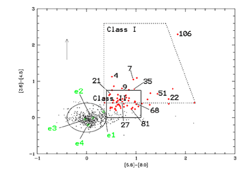
Figure 13: Colour-colour diagram for Spitzer-GLIMPSE sources in the direction of RCW 82. The ellipse shows the location of main-sequence and giant stars, the rectangle the Class II objects, and the dotted quadrilateral the area of the Class I objects, according to Allen et al. (all04 (2004)). The arrow shows the reddening shift corresponding to an extinction of $A_{V}=40$ mag.

For all these sources we used (when available) the 2MASS data (Skrutskie et al. skr06 (2006)), in order to complete the wavelength coverage and to obtain the spectral energy distributions (SEDs) of these objects. Table 2 gives the list of the sources studied in this paper. The first column gives the source designation; the second and third columns give the corresponding coordinates. Columns 4 to 6 are the 2MASS or NTT magnitudes, columns 7 to 10 are the Spitzer-GLIMPSE magnitudes, and column 11 gives the MIPS-24 $\mu$m magnitude. Sources $\#$51 and $\#$106 are saturated on the MIPS 24 $\mu$m map; we have used short exposure AKARI maps at 15 and 24 $\mu$m to measure their flux (see Zavagno et al. in preparation for a description of these data). We obtained respectively 1.97 Jy at 15 $\mu$m and 6.716 Jy at 24 $\mu$m for source $\#$51, and 3.06 Jy (15 $\mu$m) and 8.13 Jy (24 $\mu$m) for source $\#$106.

Fig. 14 shows the spatial distribution of the 63 YSOs candidates in the vicinity of RCW 82 compared to the molecular structures seen between $-42$ and $-52$ km s^-1. Several sources are seen on the borders of the H ii region and towards the ionized gas. The evolutionary stages for the 63 young sources were estimated (Class I, Class II, intermediate Class I/II) according to their position in $[3.6]-[4.5]$ versus $[5.8]-[8.0]$ diagram, in the 2MASS $J-H$ vs. $H-K_{\rm{S}}$ diagram and to their SEDs.

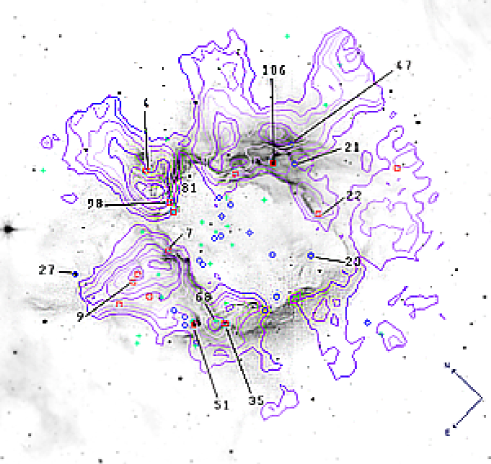
Figure 14: Superposition of the integrated ¹³CO emission contours on the 8 $\mu$m image. The selected YSOs are shown. Red squares, blue circles and green crosses respectively correspond to Class I, Intermediate and Class II sources. The sources discussed in the text are identified by their number according to Table 2.

Several sources are very luminous at mid-IR wavelengths, and have rising SEDs. Some of them have emission detected in all bands from 1.24 to 24 $\mu$m. Stars $\#$51 and $\#$68 are members of the field 1 cluster and are discussed in section 4.3.2. Star $\#$7 is from field 2 of the SofI-NTT observations and is also discussed in section 4.3.2. Source $\#$106 will be discussed in section 5.2.

Table 2: JHK, Spitzer-GLIMPSE and MIPS magnitudes of discussed stars.

Star	$\alpha_{2000}$	$\delta_{2000}$	$J$	$H$	$K_{\rm{S}}$	[3.6]	[4.5]	[5.8]	[8.0]	[24]
Objects discussed around RCW 82
4	13h 59m 34.76s	$-$61∘ 19′ 22.10′′	17.586:	15.055	12.408	10.127	8.999	8.771	8.258	5.04
9	14h 00m 01.65s	$-$61∘ 21′ 54.76′′	15.892:	15.058	12.693	9.703	8.897	8.136	7.419	4.15
21	13h 59m 01.26s	$-$61∘ 22′ 59.87′′	16.652	14.821	13.304	11.178	10.534	10.020	9.544	…
22	13h 59m 06.76s	$-$61∘ 24′ 55.77′′				13.305	12.791	11.198	9.539	…
23	13h 59m 17.56s	$-$61∘ 25′ 49.26′′	17.067:	15.109	13.574	12.150	11.611	10.902	10.043	7.48
27	14h 00m 12.63s	$-$61∘ 20′ 13.23′′	17.188:	12.422	9.390	7.040	6.611	5.932	5.205	1.85
35	13h 59m 50.89s	$-$61∘ 25′ 22.23′′	13.723	12.207	10.780	8.622	7.837	7.074	6.110	2.58
47	13h 58m 57.77s	$-$61∘ 22′ 25.58′′	16.613	14.451	12.407	10.201	9.583	9.143	8.687	…
81	13h 59m 31.91s	$-$61∘ 20′ 37.43′′	17.605	15.261	13.145	11.306	11.065	10.543	9.635	…
98	13h 59m 36.76s	$-$61∘ 20′ 48.25′′	16.267:	15.305	13.566	10.088	9.238	8.472	…	4.01
106	13h 59m 05.86s	$-$61∘ 22′ 26.50′′	…	…		10.867	8.570	6.382	4.485	…
107b	13h 59m 03.57s	$-$61∘ 22′ 15.80′′	10.870	8.074	6.320	…	…	…	…	1.47
Cluster, NTT field 1
51	13h 59m 57.61s	$-$61∘ 24′ 36.85′′	17.811a	13.795a	11.127a	8.192	7.538	6.157	4.724
68	13h 59m 57.48s	$-$61∘ 24′ 29.38′′	14.968a	12.731a	11.294a	9.671	9.304	9.123	8.116
53	13h 59m 59.94s	$-$61∘ 24′ 22.14′′	19.762a	16.419a	14.088a	11.921	11.290	10.692	10.059
36	13h 59m 58.14s	$-$61∘ 24′ 10.27′′	17.695a	14.973a	13.354a	11.353	10.819	10.245	9.626	5.64
43	13h 59m 59.16s	$-$61∘ 23′ 43.467′′	19.191a	16.308a	14.772a	13.162	12.693	12.123	11.275
102b	13h 59m 48.40s	$-$61∘ 24′ 20.23′′	15.287a	11.323a	9.341a	7.791	7.715	7.249	7.087	5.80
A2	13h 59m 57.40s	$-$61∘ 24′ 37.2′′	…	16.962a	14.216a	…	…	…	…	…
C2	13h 59m 57.12s	$-$61∘ 24′ 34.4′′	19.359a	17.381a	15.951a	…	…	…	…	…
E2	13h 59m 56.43s	$-$61∘ 24′ 29.2′′	17.865a	15.721a	14.826a	…	…	…	…	…
F2	13h 59m 56.88s	$-$61∘ 24′ 41.2′′	…	15.594a	13.889a	…	…	…	…	…
L2	13h 59m 57.89s	$-$61∘ 24′ 25.46′′	18.226a	15.828a	14.303a	12.128	11.857	11.514	…	…
M2	13h 59m 58.13s	$-$61∘ 24′ 27.07′′	…	18.989a	16.201a	13.663	12.917	…	…	…
P2	14h 00m 01.70s	$-$61∘ 24′ 51.40′′	12.126	11.7096	11.504	11.270	11.162	…	…	…
NTT field 2
A3	13h 59m 44.34s	-61∘ 22′ 43.77′′	14.099a	13.048a	12.630a	12.377	12.603	…	…	…
B3	13h 59m 44.85s	$-$61∘ 22′ 44.4′′	12.488a	12.147a	11.960a	…	…	…	…	…
C3	13h 59m 44.71s	$-$61∘ 22′ 51.1′′	…	15.172a	13.683a	…	…	…	…	…
D3	13h 59m 45.11s	$-$61∘ 22′ 46.1′′	15.578a	14.249a	13.459a	…	…	…	…	…
7	13h 59m 47.34s	$-$61∘ 22′ 01.69′′	18.766a	15.847a	14.028a	11.284	10.235	9.111	8.167	…
J3	13h 59m 46.87s	$-$61∘ 22′ 09.26′′	15.914a	14.573a	13.484a	11.882	11.445	11.381	…	…
N3	13h 59m 48.89s	$-$61∘ 23′ 03.4′′	17.606a	16.076a	14.861a	…	…	…	…	…
O3	13h 59m 49.38s	$-$61∘ 23′ 04.01′′	…	…	15.035a	12.276	11.453	10.599	…	…
candidate exciting stars
e1	13h 59m 29.93s	$-$61∘ 23′ 07.78′′	10.090	9.549	9.093	8.439	8.275	8.000	7.656	…
e2	13h 59m 29.17s	$-$61∘ 23′ 03.02′′	9.934	9.587	9.403	9.211	9.218	9.225	9.098	…
e3	13h 59m 28.11s	$-$61∘ 22′ 59.12′′	9.741	9.409	9.188	8.972	9.020	9.114	9.149	…
e4	13h 59m 27.39s	$-$61∘ 23′ 19.34′′	12.792	10.438	9.352	8.623	8.826	8.505	8.472	…

^a NTT magnitude
^b giant stars

Several sources are located in the Class I area of the $[3.6]-[4.5]$ versus $[5.8]-[8.0]$ diagram, tracing the emission of the dusty envelope in which the stars are embedded. However, Class II objects located behind a large quantity of external dust could be shifted into the Class I area of the diagram. Using 2MASS data, we constructed a $J-H$ vs. $H-K$ diagram in Fig. 15. The IR-excess evident in this diagram is generally attributed to emission from accretion disks. Characteristic SEDs of some YSOs detected around RCW 82 are shown in Fig. 16 (top and middle). In Fig. 16 (top) the SEDs of sources $\#$7, $\#$35, $\#$51 and $\#$106 are plotted. Sources $\#$4, $\#$9, and $\#$22, identified in Fig. 14, have similar SEDs increasing from 1.24 $\mu$m to 24 $\mu$m. SEDs of intermediate and Class II YSOs, such as sources $\#$21, $\#$27 (intermediate), $\#$68 and $\#$81 (Class II) have respectively SEDs which become flat or slowly decrease in the mid-IR (see Fig. 16 middle). Fig 16 (bottom) shows, for comparison, the SEDs of the four candidate exciting stars of the H ii region. Stars e2 and e3 are main-sequence stars, and e4 is most probably a giant. On this same graph we have plotted, for comparison with source e4, the SED of the source $\#$102, a typical giant star.

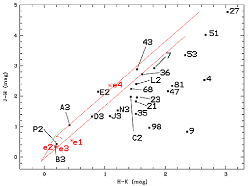
Figure 15: Colour-colour diagram with $J$, $H$ and $K_{\rm{S}}$ magnitudes (2MASS and NTT-SofI). The main sequence is plotted in red, and the giant branch in green. Reddening lines have a length corresponding to a visual extinction of 40 mag.

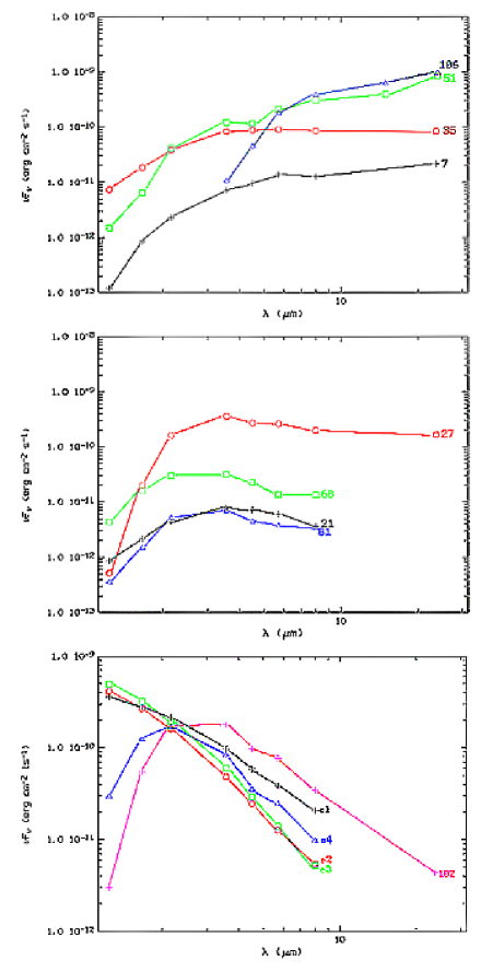
Figure 16: Spectral energy distributions of some Class I YSOs (top) and Class II and intermediate ClassI/II YSOs (middle) in the vicinity of RCW 82. The bottom image shows the SEDs of the four candidate exciting stars of the H ii region and that of star $\#$102, a typical giant.

4.3.2 The cluster

One of the two main star formation sites observed towards the borders of RCW 82 is a young cluster centred at $\alpha_{2000}$=13^h 59^m 57$.\!\!^{\rm s}$4, $\delta_{2000}$=$-$61^∘ 24^′ 32$.\!\!^{\prime\prime}$9, on the southeast border of RCW 82. Fig. 17 (middle) presents a colour composite image of this cluster. $K_{\rm{S}}$ (2.162 $\mu$m) emission observed with SofI at ESO-NTT is visible in blue, and 3.6 $\mu$m Spitzer-GLIMPSE emission in red. As for the other fields, we plotted these stars in the $J-H$ versus $H-K$ colour-colour diagram in Fig. 15. The sources are identified by their number in Table 2.

Several bright red sources, very luminous at near-IR wavelengths, are seen in this NTT field. We verified, from their magnitudes and their positions in the $J-H$ vs. $H-K$ diagram, that they are main sequence or giant stars. The small cluster at the centre of the field consists of several red stars. The sources $\#$51 and $\#$68 are the most luminous in the near-IR. Their emission dominates the emission of the cluster at longer wavelengths. MIPS 24 $\mu$m emission is centred on these sources which are not resolved.

Source $\#$51 presents a slight near-IR excess on the $J-H$ versus $H-K$ diagram (Fig. 15) and a large extinction ($A_{V}\geq$ 40 mag). According to its position on the Spitzer GLIMPSE $[3.6]-[4.5]$ vs. $[5.8]-[8.0]$ diagram (Fig. 13) this source is a Class I object, whose IR emission is dominated by an accretion envelope. The SED seen in Fig. 16 (top) clearly increases from 1.24 $\mu$m to 8 $\mu$m. The cluster is not resolved at longer wavelengths, and the flux density at 15 $\mu$m and 24 $\mu$m (AKARI data) is probably dominated by the emission of $\#$51, which is brighter and has an increasing SED up to 8 $\mu$m.

Star $\#$68 has a small near-infrared excess (Fig. 15). Its SED (Fig. 16, middle) and its position in the Spitzer-GLIMPSE colour-colour diagram (Fig. 13) are compatible with the characteristics of a Class II YSO, and thus this object may have a near-IR emission dominated by an accretion disk.

Around both these stars, SofI-NTT high resolution observations show a population of faint red sources in the cluster. Most of these sources have no Spitzer-GLIMPSE magnitudes because they are not resolved, but a diffuse emission is associated with the cluster at these wavelengths. Sources C2 and L2 appear in the colour-colour diagram (Fig. 15) with a small near-IR excess, and could be YSOs. In contrast, the colours of E2 suggest it is a giant star.

Source P2 is located southeast of the cluster and is clearly associated with a bow-shock (see Fig. 17 (middle)). According to its near-IR magnitudes this object is a main sequence star of type $\sim$B3V if located at the distance of RCW 82, and associated with 3.5 mag of visual extinction. Moreover only a spectrum could confirm its characteristics. This bow shock may originate from a wind emitted by source P2 and interacting with material flowing away from the cluster (more or less in the direction of the cluster). Another possibility is that star P2 emits a wind and is moving in the ambient medium, creating the bow shock (Povich et al. pov08 (2008)). Complementary data are needed to distinguish between the two possibilities. However, the first one is favored by the good alignment between the vertex of the bow shock and the direction of the cluster.

Northeast of the young cluster, three other bright red sources are seen (sources $\#$36, $\#$53 and the “Giant”). Sources $\#$36 and $\#$53 are classified as intermediate Class I/II sources from the colour-colour GLIMPSE diagram. This is in agreement with their SEDs and with their positions in the $JHK$ colour-colour diagram. The third source has the near-IR colours of a giant star.

4.3.3 Field 2

Field 2, presented in Fig. 17 (bottom), is centred on a bright border at $\alpha_{2000}$=13^h 59^m 45$.\!\!^{\rm s}$6, $\delta_{2000}$=$-$61^∘ 22^′ 54$.\!\!^{\prime\prime}$5. This field contains a bright filament at 8.0 $\mu$m – a part of the hot PDR bordering RCW 82, with a structure pointing towards the exciting stars (Fig. 5). Several stellar objects are seen in the direction of this structure, more or less embedded in the diffuse filamentary emission.

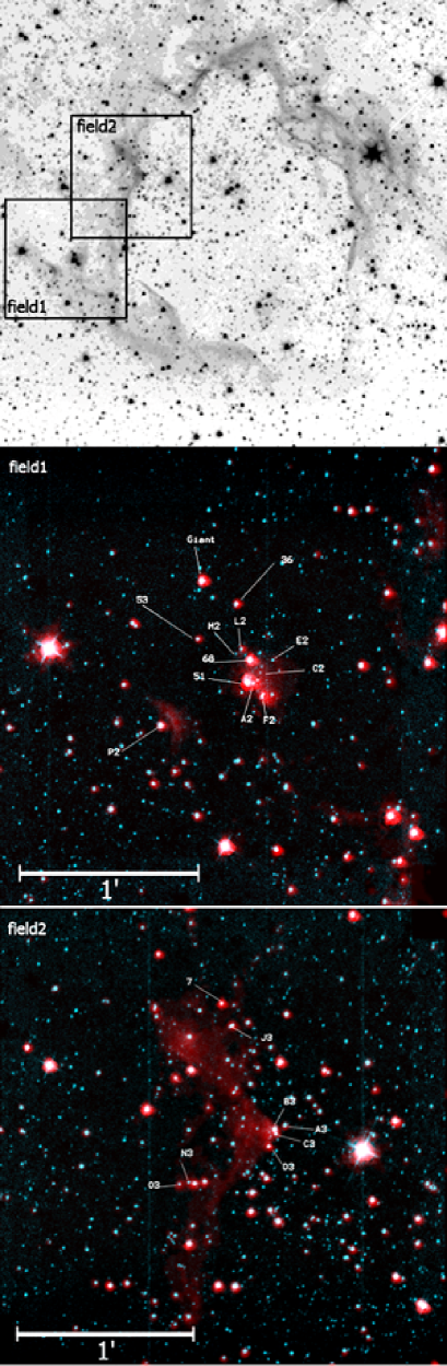
Figure 17: Top: RCW 82 at 3.6 $\mu$m, logarithmic scale. Middle and Bottom: Colour composite image of field1 and field2. NTT $K_{\rm{S}}$ emission is in blue, and Spitzer-GLIMPSE emission at 3.6 $\mu$m in red. The coordinates of the image centres are $\alpha_{2000}$=13^h59^m 57$.\!\!^{\rm s}$4, $\delta_{2000}$=$-$61^∘ 24^′ 32$.\!\!^{\prime\prime}$9 (field1) and $\alpha_{2000}$=13^h 59^m 45$.\!\!^{\rm s}$6, $\delta_{2000}$=$-$61^∘ 22^′ 54$.\!\!^{\prime\prime}$5. The field sizes are 2$.\mkern-4.0mu^{\prime}$6$\times$2$.\mkern-4.0mu^{\prime}$6. North is to up and east is left.

Only the most interesting objects are identified on Fig. 17 (bottom). Most sources of the field are main sequence or giant stars. Source C3 seems to correspond to the tip of the structure seen at 8 $\mu$m and at 24 $\mu$m. This source has been measured in $H$ and $K_{\rm{S}}$. It is seen in $J$, but not measured because it lies too close to star B3, which is more luminous and probably a main sequence star. We used a source of similar brightness, more isolated and measured in $J$ (17.67 mag) to estimate the position of the source C3 on the $J-H$ vs. $H-K_{\rm{S}}$ diagram; this indicates a young star. Moreover, C3 continues to be visible at longer wavelengths, up to 24 $\mu$m, even if no Spitzer-GLIMPSE magnitudes are available.

Other candidate YSOs are sources $\#$7, J3 and N3. Source O3 has missing measurements in the near- and mid-IR which prevents us from determining its nature. In addition we confirmed that the two sources to the right of sources O3 and N3 have main sequence near-IR colours.

5 Discussion

5.1 The molecular material

Fig.12 shows that the H₂ column densities reach values up to about 3$\times$10²² cm^-2. The four densest condensations are seen north of RCW 82. The layer of neutral material collected during the expansion of the H ii region is clearly seen in this figure.

Fig. 18 shows a composite colour image of RCW 82 with the H$\alpha$ emission in turquoise and the integrated ¹³CO emission between $-42$ and $-52$ km s^-1 in red. It shows that the ionized gas seems to escape from the centre of RCW 82, flowing between condensations $\#$1 and $\#$2, and between $\#$1 and $\#$5. We also see H$\alpha$ emission between the collected layer of accumulated material (structure $\#$7) and the dense condensations $\#$5 and $\#$6. This point is important because it demonstrates that the most massive fragments seen at the border of RCW 82 are adjacent to the H ii region and thus submitted to the pressure of the ionized gas.

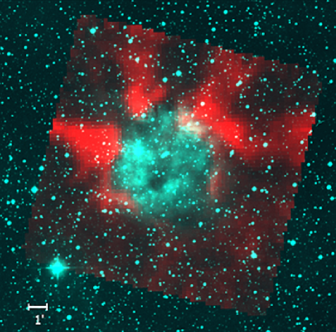
Figure 18: Colour composite image of RCW 82. H$\alpha$ emission of the ionized gas is seen in turquoise, and the molecular material associated with the H₂ column density map (see Fig. 12) in red.

One of the characteristics of the molecular emission around RCW 82 is the shape of the condensations. They present a bright core adjacent to the ionized region and extended diffuse tails almost perpendicular to the ionization front. These structures are seen in the ¹²CO and ¹³CO maps. We can only speculate about the origin of these structures: i) the exciting cluster of RCW 82 formed at the meeting point of several filaments, and what we see is the remnant of these pre-existing filaments; ii) the H ii region formed and evolved in a medium with pre-existing dense condensations. The expanding H ii region interacted with these condensations, collecting more material in their direction, hence the dense cores adjacent to the ionized gas. Then the ionized gas escaped from the central H ii region in directions of lower density zones, giving a radial shape to the molecular material hidden behind the heads of the condensations.

Also RCW 82 is seen on the border of a large bubble, to which it is possibly linked. The molecular component observed around $-55$ km s^-1 has a velocity compatible with the velocity of the H$\alpha$ emission of RCW 82 and show filaments following the borders of the large shell. The large shell has possibly triggered the formation of RCW 82 or is in interaction with the neutral material surrounding RCW 82.

5.2 Star formation around RCW 82

5.2.1 The distribution of YSOs

Fig. 19 shows the distribution of the YSOs detected in the direction of RCW 82, superimposed on the ¹³CO emission integrated between $-42$ and $-52$ km s^-1. This image shows a strong correlation between Class I sources and the molecular emission surrounding the H ii region. Many of these sources are not observed in the direction of molecular emission peaks, but are located on the borders of the condensations. However we have to keep in mind that some sources are possibly linked with molecular material observed in other velocity ranges.

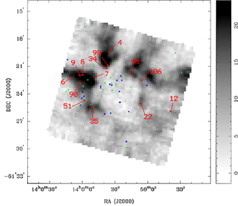
Figure 19: Map of the ¹³CO emission integrated between $-42$ and $-52$ km s^-1. Red squares, blue circles and green crosses represent the positions of Class I, intermediate, and Class II YSOs, respectively.

YSOs $\#$34 and $\#$98 are situated on the border of the molecular structure $\#$1a, linked to RCW 82. Only molecular emission associated with the H ii region (see Fig. 8) is observed in the direction of these two sources, so there is a strong probability that they are both linked to the H ii region.

Three other sources are very probably linked to the collected layer of material surrounding RCW 82. These sources are $\#$48, $\#$106 and $\#$22. They are perfectly aligned along the western part of the collected layer (fragment $\#$7), and no molecular emission at other velocities is seen in their direction.

Another interesting source is the Class I $\#$35. Molecular emissions at velocities $-55$, $-35$ and $+16$ km s^-1 are detected in the direction of this young source, but the strongest emission corresponds to the structure $\#$3 which is associated with RCW 82. Thus this Class I YSO could have been triggered by the H ii region.

5.2.2 The most massive YSOs

We continue this discussion by focusing on the two main sites of star formation seen on the borders of the H ii region.

Source $\#$106, an isolated YSO:

The association of this source with RCW 82 is highly probable. It is seen in the direction of the collected layer of materiel in ¹²CO and ¹³CO (structure $\#$7 on Fig. 12), on the western side of RCW 82. No other molecular emission is associated with source $\#$106 on the line of sight. Thus it is highly probable that this YSO is linked to RCW 82 and that its formation was triggered by the expansion of the H ii region.

Our study in the mid-IR shows that source $\#$106 could be a Class I candidate (Fig. 13). Furthermore this object seems to be massive according to its SED (Fig. 16), and appears to be isolated. This point is confirmed by some GEMINI 10 $\mu$m and 18.3 $\mu$m observations on which source $\#$106 appears as a single stellar object (Zavagno et al. in preparation).

Source $\#$106, corresponding to the MSX point source G310.9438+00.4411, was observed by Urquhart et al. (urq07 (2007)) at 3 cm and 6 cm. Their non-detection (at a 4$\sigma$ level of 1.1 mJy at 6 cm) allows us to derive an upper limit for the number of ionizing photons emitted by this source, using the relation (1) of Simpson & Rubin (sim90 (1990)). Assuming that star $\#$106 is probably not hot enough to ionize helium and adopting $T_{\rm{e}}$=10000 K we obtain $\log(N_{\rm{Lyc}}$)$\sim$45 s^-1. Thus, according to Smith et al. (smi02 (2002)), YSO $\#$106 cannot contain a central source hotter than a B1.5 star.

We used the online fitting tool of Robitaille et al. (rob07 (2007), http://caravan.astro.wisc.edu/protostars/) to model the SED of this source. We used data from Spitzer-GLIMPSE 3.6 $\mu$m to MIPS 70 $\mu$m (this last measurement is highly uncertain due to the underlying emission of the PDR). Most of the models show a massive and dominant disk: considering the 50 first best models the disk’s mass is high and can reach 0.26 $M_{\odot}$; also in most cases the envelope accretion rate is zero or very small. Another important conclusion is that the central object is massive, between 7 and 18 $M_{\odot}$. The inclination angle and the extinctions (both interstellar and circumstellar) are poorly constrained.

Two remarks can be made: i) models with important and dominant disks are compatible with the presence of the strong silicate absorption feature seen on the GEMINI spectra of the source (Zavagno et al. in preparation) This absorption feature indicates that source $\#$106 has a disk which is seen nearly edge-on; ii) masses of more than 10 $M_{\odot}$ for the central source are incompatible with the non-detection of radio emission at 3 and 6 cm by Urquhart et al. (urq07 (2007)).

Thus source $\#$106 is probably a Class II source containing a massive central object. Whitney et al. (whi04 (2004)) shown a trend for higher temperature sources to be redder, especially [3.6]-[4.5], than the colours usually attributed to Class II sources (the box in Fig. 13); a Class II YSO with a hot central source can be mistaken for a Class I source. Thus the mass of the central source of $\#$106 and the hypothetical presence of an accreting envelope remain to be ascertained.

The cluster:

The second main site of star formation in the direction of RCW 82 is the young cluster at the eastern border of the H ii region. The brightest star at mid-IR wavelengths, source $\#$51, is centred on the MSX point source G311.0341+00.3791. This was also observed by Urquhart et al. (urq07 (2007)) at 3 cm and 6 cm, but no radio continuum emission was detected. As for star $\#$106, this means that no star massive enough to ionize hydrogen is present in this cluster.

Fig. 19 shows that the cluster lies in a region of low molecular emission, slightly at the back of the collected layer, thus rather far away from the ionization front. Fig. 20 is the calculated $N(\rm{H_{2}}$) map based on the ¹³CO and ¹²CO emission integrated between $-56.6$ and $-52.8$ km s^-1. The position of source $\#$51 is shown, in the direction of a massive condensation. Thus the young cluster may be associated with this molecular structure. In conclusion, the association of the cluster with RCW 82 is uncertain, depending on the association of the molecular emission seen around $-55$ km s^-1 with RCW 82.

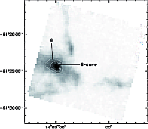
Figure 20: N(H₂) map of the molecular emission integrated between $-56.6$ and $-52.8$ km s^-1. The contours correspond to the levels of 1.5 $\times$ 10²² cm^-2 and 2 $\times$ 10²² cm^-2 used to compute the mass of the condensation (Tab. 1). The position of the Class I $\#$51 is shown by a white cross.

5.3 Comparisons with models

In the following we estimate the age of RCW 82, to see if the collect & collapse process is possibly at work around this region. We will assume that RCW 82 formed and evolved in a homogeneous medium of density $n_{0}$.

If we use an ionizing photon flux of 9.0 $\times$ 10⁴⁸ s^-1 (or 4.6 $\times$ 10⁴⁸ s^-1 for the exciting star (Sect. 2.2), a present radius of 3 pc for the H ii region, and assume $n_{0}$=10³ atoms cm^-3 (this value will be justified a posteriori), we estimate a present electron density for the H ii region n${}_{e}\sim$120 cm^-3 (90 cm^-3), a mass M(H ii)=310 $M_{\odot}$ (230 $M_{\odot}$), an expansion velocity $\sim$3.7 km s^-1 (3.2 km s^-1), and an age $\sim$0.4 Myr (0.5 Myr).

The sphere of 3 pc radius initially contained 2600$M_{\odot}$ of material. This material is now to be found in the ionized region and in the shell of material accumulated around the ionized gas; thus a mass $\sim$ 2260$M_{\odot}$ (2370$M_{\odot}$) for this shell, in rather good agreement with the total mass ($\sim$2520$M_{\odot}$) of the structures adjacent to the IF ($\#$3, $\#$2-core, $\#$1a, $\#$1b and $\#$7; these structures are considered as parts of the collected layer); hence the justification of the adopted value for n₀.

We can now, according to Whitworth et al. (whi94 (1994), section 5), estimate when the fragmentation of this collected layer should occur. Assuming $a_{\rm{S}}$=0.2 km s^-1 for the turbulent velocity in the collected layer, we find that the fragmentation of the H ii region occurs 1.6 Myr after its formation, when its radius is 5.74 pc. The fragmentation will be later, and for larger radii, for higher values of $a_{\rm{S}}$. We conclude that RCW 82 is not old enough for star formation to take place in the collected layer via the collect & collapse process.

The formation of the YSOs present on the border of RCW 82 most probably results from some other process of star formation like small-scale Jeans gravitational instabilities in the collected layer, or interactions of the IF with pre-existing condensations (Lefloch & Lazareff lef94 (1994)).

6 Conclusions

We have presented a multi-wavelength study of the H ii region RCW 82. Molecular observations in ¹²CO and ¹³CO obtained with Mopra and the near-to-mid IR study of YSOs in the direction of this star forming region allow us to make the following conclusions:

$\bullet$ RCW 82 is seen on the border of a large shell observed at 8 $\mu$m, which probably surrounds an H ii region. Unfortunately the spatial coverage of our molecular observations is not sufficient to prove the link between the two regions;

$\bullet$ We have identified four candidate exciting stars of RCW 82. Among these sources, stars $\#$e2 and $\#$e3 are probably O-type stars responsible for the ionization of RCW 82;

$\bullet$ Molecular material is associated with RCW 82. We observe a molecular layer around the H ii region, corresponding to interstellar material accumulated around the ionized gas during the expansion of RCW 82. We also observe elongated structures, oriented almost perpendicular to the ionization front. We suggest that these structures correspond to pre-existing condensations, possibly shaped by UV radiation. Some condensations have masses greater than 2000 $M_{\odot}$;

$\bullet$ Many YSOs are observed at the periphery of RCW 82, among which is a non-negligible number of potential Class I sources. Their distribution is not uniform and most of them are observed on the borders of RCW 82, close to the IF. It indicates that triggered star formation is at work around this H ii region;

$\bullet$ The presence of a collected layer of material around RCW 82 shows that the collect part of the collect and collapse process has occurred. However, our age estimate of RCW 82 shows that the H ii region is probably not evolved enough for the collected shell to be in the fragmentation phase. This means that the star formation activity observed around RCW 82 is due to other processes;

$\bullet$ Among the YSOs we have identified a candidate isolated massive young object, source $\#$106; its evolutionary stage remains to be more precisely defined. The formation of this object may have been triggered by RCW 82, as it is observed in the direction of the shell of material collected around the H ii region. However this point remains to be confirmed as the estimated age of the H ii region does not allow enough time for the collapse process to occur. On the other hand, the young cluster, observed around source $\#$51, could be associated with a massive molecular component observed around $-55$ km s^-1, for which the association with RCW 82 is uncertain.

- (1) Allen, L.E., Calvet, N., D’Alessio, P., Merin, B., Hartmann, L., Megeath, S.T., Gutermuth, R.A., Muzerolle, J. Pipher, J.L., Myers, P.C., Fazio, G.G., 2004, ApJS, 154, 363
- (2) Bains, I.; Wong, T.; Cunningham, M.; Sparks, P.; Brisbin, D.; Calisse, P.; Dempsey, J. T. et al. 2006, MNRAS, 367, 1609
- (3) Benjamin, R.A., Churchwell, E., Babler, B.L., Bania, T.M., Clemens, D.P., Cohen, M., Dickey, J.M., Indebetouw, R., Jackson, J.M., Kobulnicky, H.A. et al. 2003, PASP, 115, 953
- (4) Bock, D.C.-J., Large, M.I., & Sadler, E.M. 1999, AJ, 117, 1578
- (5) Bonnarel, F., Fernique, P., Bienayme, O., Egret, D., Genova, F., Louys, M., Ochsenbein, F.,Wenger, M., Bartlett, J.G. 2000, A&ASS, 143, 33
- (6) Brand, J., Blitz, L., 1993, A&A, 275, 67
- (7) Cappa, C., Niemela, V.S., Amorin, R., Vasquez, J. 2008, A&A, 477, 173
- (8) Carey, S.J., Noriega-Crespo, A., Price, S.D., et al. 2005, BAAS, 37, 1252
- (9) Caswell, J.L., Haynes, R.F., 1987, A&A, 171, 261
- (10) Churchwell, E., Povich, M. S., Allen, D., et al. 2006, ApJ, 649, 759
- (11) Cohen, M., & Green, A.J. 2001, MNRAS, 325, 531
- (12) Cohen, M., Green, A.J., Meade, M.R., et al. 2007, MNRAS, 374, 979
- (13) Crété, E., Giard, M., Joblin, C., Vauglin, I., Léger, A., & Rouan, D. 1999, A&A, 352, 277
- (14) Deharveng, L., Lefloch, B., Zavagno, A., Caplan, J., Whitworth, A.P., Nadeau, D., Martin, S., 2003, A&A, 408, L25
- (15) Deharveng, L., Zavagno, A., Caplan, J. 2005, A&A, 433, 565: paper I
- (16) Deharveng, L.; Lefloch, B.; Kurtz, S.; Nadeau, D.; Pomars, M.; Caplan, J.; Zavagno, A. 2008, A&A, 482, 585
- (17) Elmegreen, B. G., Lada, C.J. 1977, ApJ, 214, 725
- (18) García-Segura, G., Franco, J. 1996, ApJ, 469, 171
- (19) Georgelin, Y. M., Amram, P., Georgelin, Y. P., Le Coarer, E., Marcelin, M. 1994 A&AS, 108, 513
- (20) Goudis, C., Meaburn, J. 1978, A&A 68, 189
- (21) Haynes, R. F.; Caswell, J. L.; Simons, L. W. J. 1979, AuJPA, 48, 1
- (22) Hunter, D. 1994, AJ, 107, 565
- (23) Jones, P. A.; Burton, M. G.; Cunningham, M. R.; Menten, K. M.; Schilke, P.; Belloche, A.; Leurini, S.; Ott, J.; Walsh, A. J. 2008, MNRAS, 386, 117
- (24) Kirsanova, M.S., Sobolev, A.M., Thomasson, M., Wiebe, D.S., Johansson, L.E.B., Seleznev, A.F. 2008, MNRAS, in press (arXiv:0805.1586v1)
- (25) Kuchar, T. A. & Clark, F. O. 1997, ApJ, 488, 224
- (26) Ladd, N., Purcell, C., Wong, T. Robertson, S. 2005, Publ. Astron. Soc. Aust., 22, 62
- (27) Lefloch, B., Lazareff, B., 1994 A&A, 289, 559
- (28) Léger, A., Puget, J.-L. 1984, A&A, 137, L5
- (29) Martins, F., Schaerer, D., Hillier, D.J., 2005, A&A, 436, 1049
- (30) McClure-Griffiths, N.M., Green, A. J., Dickey, J. M., Gaensler, B. M., Haynes, R. F., Wieringa, M. H. 2001, ApJ, 551, 394
- (31) Meaburn, J. 1979, A&A, 75, 127
- (32) Müller, H. S. P., Schlöder, F., Stutzki, J. and Winnewisser, G.2005, J. Mol. Struct. 742, 215
- (33) Osterbrock, D.E. 1957, ApJ, 125, 622
- (34) Parker, Q.A., Phillipps, S., Pierce, M. J., Hartley, M., Hambly, N. C., Read, M. A., MacGillivray, H. T., Tritton, S. B., Cass, C. P., Cannon, R. D., et al. 2005, MNRAS, 362, 689
- (35) Peeters, E., Martín-Hernández, N.L., Damour, F., et al. 2002, A&A, 381, 571
- (36) Povich, M. S., Benjamin, R. A., Whitney, B. A., Babler, B. L., Indebetouw, R., Meade, M. R., Churchwell, E. 2008, arXiv0808.2168P
- (37) Price, S.D., Egan, S.M., Carey, S.J., Mizuno, D.R., Kuchar, T.A. 2001, AJ, 121, 2819
- (38) Robitaille, T.P., Whitney, B.A., Indebetouw, R., Wood, K. 2007, ApJS, 169, 328
- (39) Rodgers, A. W., Campbell, C. T., Whiteoak, J. B. 1960, MNRAS, 121, 103
- (40) Rosolowsky, E., Leroy, A. 2006, PASP, 118, 590
- (41) Russeil, D., Georgelin, Y. M., Amram, P., Gach, J. L., Georgelin, Y. P., Marcelin, M. 1998, A&AS, 130,119
- (42) Sault, R. J.; Teuben, P.J.; Wright, M. C. H. 1995, “A retrospective view of Miriad” in Astronomical Data Analysis Software and Systems IV, ed. R. Shaw, H. E. Payne, J. J. E. Hayes, ASP Conf. Ser., 77, 433-436
- (43) Simpson, J.P., Rubin, R.H. 1990, ApJ, 354, 165
- (44) Skrutskie, M.F., Cutri, R.M., Stiening, R., Weinberg, M. D., Schneider, S., Carpenter, J. M., Beichman, C., Capps, R., Chester, T., Elias, J. et al. 2006, AJ, 131, 1163
- (45) Smith, L., Norris, R.P.F., Crowther, P.A. 2002, MNRAS, 337, 1309
- (46) Stetson, P.B. 1987, PASP, 99, 191
- (47) Urquhart, S. J., Busfield, A. L. , Hoare, M. G., Lumsden, S. L., Clarke A. J., Moore, T. J. T., Mottram, J. C., and Oudmaijer, R. D. 2007, A&A, 461, 11
- (48) van Dishoeck, E. F.; Glassgold, A. E.; Guelin, M.; Jaffe, D. T.; Neufeld, D. A.; Tielens, A. G. G. M.; Walmsley, C. M.1992, IAUS, 150, 285
- (49) Watson, C., Povich, M.S., Churchwell, E.B., Babler, B.L., Chunev, G., Hoare, M., Indebetouw, R., Meade, M.R., Robitaille, T.P., Whitney, B.A. 2008, ApJ, 681, 1341
- (50) Whitney, B.A., Indebetouw R., Bjorkman, J.E., Wood, K. 2004, ApJ, 617, 1177
- (51) Whitworth, A.P., Bhattal, A.S., Chapman, S.J., Disney, M. J., Turner, J.A. 1994, MNRAS, 268, 291
- (52) Zavagno, A., Deharveng, L., Comeron, F., Brand, J., Massi, F. et al. 2006, A&A, 446, 171
- (53) Zavagno, A., Pomarès, M., Deharveng, L., Hosokawa, T., Russeil, D., Caplan, J. 2007, A&A, 472, 835