Asset Allocation and Risk Assessment with Gross Exposure Constraints for Vast Portfolios

Abstract

Markowitz (1952, 1959) laid down the ground-breaking work on the mean-variance analysis. Under his framework, the theoretical optimal allocation vector can be very different from the estimated one for large portfolios due to the intrinsic difficulty of estimating a vast covariance matrix and return vector. This can result in adverse performance in portfolio selected based on empirical data due to the accumulation of estimation errors. We address this problem by introducing the gross-exposure constrained mean-variance portfolio selection. We show that with gross-exposure constraint the theoretical optimal portfolios have similar performance to the empirically selected ones based on estimated covariance matrices and there is no error accumulation effect from estimation of vast covariance matrices. This gives theoretical justification to the empirical results in Jagannathan and Ma (2003). We also show that the no-short-sale portfolio is not diversified enough and can be improved by allowing some short positions. As the constraint on short sales relaxes, the number of selected assets varies from a small number to the total number of stocks, when tracking portfolios or selecting assets. This achieves the optimal sparse portfolio selection, which has close performance to the theoretical optimal one. Among 1000 stocks, for example, we are able to identify all optimal subsets of portfolios of different sizes, their associated allocation vectors, and their estimated risks. The utility of our new approach is illustrated by simulation and empirical studies on the 100 Fama-French industrial portfolios and the 400 stocks randomly selected from Russell 3000.

Keywords: Short-sale constraint, mean-variance efficiency, portfolio selection, risk assessment, risk optimization, portfolio improvement.

1 Introduction

Portfolio selection and optimization has been a fundamental problem in finance ever since Markowitz (1952, 1959) laid down the ground-breaking work on the mean-variance analysis. Markowitz posed the mean-variance analysis by solving a quadratic optimization problem. This approach has had a profound impact on the financial economics and is a milestone of modern finance. It leads to the celebrated Capital Asset Pricing Model (CAPM), developed by Sharpe (1964), Lintner (1965) and Black (1972). However, there are documented facts that the Markowitz portfolio is very sensitive to errors in the estimates of the inputs, namely the expected return and the covariance matrix. One of the problems is the computational difficulty associated with solving a large-scale quadratic optimization problem with a dense covariance matrix (Konno and Hiroaki, 1991). Green and Hollified (1992) argued that the presence of a dominant factor would result in extreme negative weights in mean-variance efficient portfolios even in the absence of the estimation errors. Chopra and Ziemba (1993) showed that small changes in the input parameters can result in large changes in the optimal portfolio allocation. Laloux et al.(1999) found that Markowitz’s portfolio optimization based on a sample covariance matrix is not adequate because its lowest eigenvalues associated with the smallest risk portfolio are dominated by estimation noise. These problems get more pronounced when the portfolio size is large. In fact, Jagannathan and Ma (2003) showed that optimal no-short-sale portfolio outperforms the Markowitz portfolio, when the portfolio size is large.

To appreciate the challenge of dimensionality, suppose that we have 2,000 stocks to be allocated or managed. The covariance matrix alone involves over 2,000,000 unknown parameters. Yet, the sample size $n$ is usually no more than 400 (about two-year daily data, or eight-year weekly data, or thirty-year monthly data). Now, each element in the covariance matrix is estimated with the accuracy of order $O(n^{-\frac{1}{2}})$ or 0.05. Aggregating them over millions of estimates in the covariance matrix can lead to devastating effects, which can result in adverse performance in the selected portfolio based on empirical data. As a result, the allocation vector that we get based on the empirical data can be very different from the allocation vector we want based on the theoretical inputs. Hence, the mean-variance optimal portfolio does not perform well in empirical applications, and it is very important to find a robust portfolio that does not depend on the aggregation of estimation errors.

Several techniques have been suggested to reduce the sensitivity of the Markowitz-optimal portfolios to input uncertainty. Chopra and Ziemba (1993) proposed a James-Stein estimator for the means and Ledoit and Wolf (2003, 2004) proposed to shrink a covariance matrix towards either the identity matrix or the covariance matrix implied by the factor structure, while Klein and Bawa (1976) and Frost and Savarino (1986) suggested Bayesian estimation of means and covariance matrix. Fan et al.(2008) studied the covariance matrix estimated based on the factor model and demonstrated that the resulting allocation vector significantly outperforms the allocation vector based on the sample covariance. Pesaran and Zaffaroni (2008) investigated how the optimal allocation vector depends on the covariance matrix with a factor structure when portfolio size is large. However, these techniques, while reducing the sensitivity of input vectors in the mean-variance allocation, are not enough to address the adverse effect due to the accumulation of estimation errors, particularly when portfolio size is large. Some of theoretical results on this aspect have been unveiled by Fan et al.(2008).

Various efforts have been made to modify the Markowitz unconstrained mean-variance optimization problem to make the resulting allocation depend less sensitively on the input vectors such as the expected returns and covariance matrices. De Roon et al.(2001) considered testing-variance spanning with the no-short-sale constraint. Goldfarb and Iyengar (2003) studied some robust portfolio selection problems that make allocation vectors less sensitive to the input vectors. The seminal paper by Jagannathan and Ma (2003) imposed the no-short-sale constraint on the Markowitz mean-variance optimization problem and gave insightful explanation and demonstration of why the constraints help even when they are wrong. They demonstrated that their constrained efficient portfolio problem is equivalent to the Markowitz problem with covariance estimated by the maximum likelihood estimate with the same constraint. However, as demonstrated in this paper, the optimal no-short-sale portfolio is not diversified enough. The constraint on gross exposure needs relaxing in order to enlarge the pools of admissible portfolios. We will provide statistical insights to the question why the constraint on gross exposure prevents the risks or utilities of selected portfolios from accumulation of statistical estimation errors. This is a prominent contribution of this paper in addition to the utilities of our formulation in portfolio selection, tracking, and improvement. Our result provides a thoeretical insight to the phenomenon, observed by Jagannathan and Ma (2003), why the wrong constraint helps on risk reduction for large portfolios.

We approach the utility optimization problem by introducing a gross-exposure constraint on the allocation vector. This makes not only the Markowitz problem more practical, but also bridges the gap between the no-short-sale utility optimization problem of Jagannathan and Ma (2003) and the unconstrained utility optimization problem of Markowitz (1952, 1959). As the gross exposure parameter relaxes from 1 to infinity, our utility optimization progressively ranges from no short-sale constraint to no constraint on short sales. We will demonstrate that for a wide range of the constraint parameters, the optimal portfolio does not sensitively depend on the estimation errors of the input vectors. The theoretical (oracle) optimal portfolio and empirical optimal portfolio have approximately the same utility. In addition, the empirical and theoretical risks are also approximately the same for any allocation vector satisfying the gross-exposure constraint. The extent to which the gross-exposure constraint impacts on utility approximations is explicitly unveiled. These theoretical results are demonstrated by several simulation and empirical studies. They lend further support to the conclusions made by Jagannathan and Ma (2003) in their empirical studies.

To better appreciate the above arguments, the actual risk of a portfolio selected based on the empirical data can be decomposed into two parts: the actual risk (oracle risk) of the theoretically optimal portfolio constructed from the true covariance matrix and the approximation error, which is the difference between the two. As the gross-exposure constraint relaxes, the oracle risk decreases. When the theoretical portfolio reaches certain size, the marginal gain by including more assets is vanishing. On the other hand, the risk approximation error grows quickly when the exposure parameter is large for vast portfolios. The cost can quickly exceed the benefit of relaxing the gross-exposure constraint. The risk approximation error is maximized when there is no constraint on the gross-exposure and this can easily exceed its benefit. On the other hand, the risk approximation error is minimized for the no-short-sale portfolio, and this can exceed the cost due to the constraint.

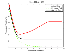
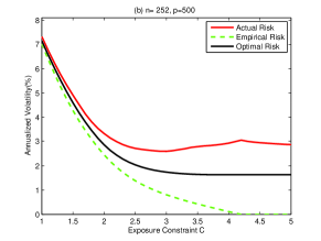
Figure 1: The risks of theoretically optimal portfolios, and the actual risks of the empirically optimal portfolios, and the empirical risks of the empirically optimal portfolios under gross-exposure constraints are plotted against the gross-exposure parameter $c$. The data are based simulated 252 daily returns of 500 stocks from the Fama-French three-factor model. As the gross-exposure parameter $c$ increases, the discrepancy between the optimal risks, actual risks, empirical risks get larger, which means the actual risk might be quite far away from the risk we think it should be. The total number of stocks under consideration is (a) 200 and (b) 500.

The above arguments can be better appreciated by using Figure 1, in which 252 daily returns for 500 stocks were generated from the Fama-French three-factor model, detailed in Section 4. We use the simulated data, instead of the empirical data, as we know the actual risks in the simulated model. The risks of optimal portfolios stop to decreases further when the gross exposure constant $c\geq 3$. On the other hand, based on the sample covariance matrix, one can find the empirically optimal portfolios with gross-exposure constraint $c$. The empirical risk and actual risk start to diverge when $c\geq 2$. The empirical risks are overly optimistic, reaching zero for the case of 500 stocks with one year daily returns. On the other hand, the actual risk increases with the gross exposure parameter $c$ until it reaches its asymptote. Hence, the Markowitz portfolio does not have the optimal actual risk.

Our approach has important implications in practical portfolio selection and allocation. Monitoring and managing a portfolio of many stocks is not only time consuming but also expensive. Therefore, it is ideal to pick a reasonable number of assets to mitigate these two problems. Ideally, we would like to construct a robust portfolio of reasonably small size to reduce trading, re-balancing, monitoring, and research costs. We also want to control the gross exposure of the portfolio to avoid too extreme long and short positions. However, to form all optimal subsets of portfolios of different sizes from a universe of over 2,000 (say) assets is an NP-hard problem if we use the traditional best subset approach, which cannot be solved efficiently in feasible time. Our algorithm allows one to pick an optimal subset of any number of assets and optimally allocate them with gross-exposure constraints. In addition, its associated utility as a function of the number of selected assets is also available so that the optimal number of portfolio allocations can be chosen.

2 Portfolio optimization with gross-exposure constraints

Suppose we have $p$ assets with returns $R_{1}$, $\cdots,R_{p}$ to be managed. Let R be the return vector, $\Sigma$ be its associated covariance matrix, and w be its portfolio allocation vector, satisfying $\mbox{\bf w}^{T}\mbox{\bf 1}=1$. Then the variance of the portfolio return $\mbox{\bf w}^{T}\mbox{\bf R}$ is given by $\mbox{\bf w}^{T}\mbox{\boldmath$\Sigma$}\mbox{\bf w}$.

2.1 Constraints on gross exposure

Let $U(\cdot)$ be the utility function, and $\|\mbox{\bf w}\|_{1}=|w_{1}|+\cdots+|w_{p}|$ be the $L_{1}$ norm. The constraint $\|\mbox{\bf w}\|_{1}\leq c$ prevents extreme positions in the portfolio. A typical choice of $c$ is about 1.6, which results in approximately 130% long positions and 30% short positions. When $c=1$, this means that no short sales are allowed as studied by Jagannathan and Ma (2003). When $c=\infty$, there is no constraint on short sales. As a generalization to the work by Markowitz (1952) and Jagannathan and Ma (2003), our utility optimization problem with gross-exposure constraint is

$$\max_{\mbox{\bf w}} E[U(\mbox{\bf w}^{T}\mbox{\bf R})]$$

$$s.t. \mbox{\bf w}^{T}\mathbf{1}=1,\>\>\|\mbox{\bf w}\|_{1}\leq c,\>\>\mbox{\bf A}\mbox{\bf w}=\mbox{\bf a}.$$

The utility function can also be replaced by any risk measures such as those in Artzner et al.(1999), and in this case the utility maximization should be risk minimization.

As to be seen shortly, the gross-exposure constraint is critical in reducing the sensitivity of the utility function on the estimation errors of input vectors such as the expected return and covariance matrix. The extra constraints $\mbox{\bf A}\mbox{\bf w}=\mbox{\bf a}$ are related to the constraints on percentage of allocations on each sector or industry. It can also be the constraint on the expected return of the portfolio.

The $L_{1}$ norm constraint has other interpretations. For example, $\|\mbox{\bf w}\|_{1}$ can be interpreted as the transaction cost. In this case, one would subtract the term $\lambda\|\mbox{\bf w}\|_{1}$ from the expected utility function, resulting in maximizing the modified utility function

$$\max_{\mbox{\bf w}}E[U(\mbox{\bf w}^{T}\mbox{\bf X})]-\lambda\|\mbox{\bf w}\|_{1}.$$

This is equivalent to problem (2.1).

The question of picking a reasonably small number of assets that have high utility arises frequently in practice. This is equivalent to impose the constraint $\|\mbox{\bf w}\|_{0}\leq c$, where $\|\mbox{\bf w}\|_{0}$ is the $L_{0}$-norm, counting number of non-vanishing elements of w. The utility optimization with $L_{0}$-constraint is an NP-complete numerical optimization problem. However, replacing it by the $L_{1}$ constraint is a feasible convex optimization problem. Donoho and Elad (2003) gives the sufficient conditions under which two problems will yield the same solution.

2.2 Utility and risk approximations

It is well known that when the return vector $\mbox{\bf R}\sim N(\mbox{\boldmath$\mu$},\mbox{\boldmath$\Sigma$})$ and $U(x)=1-\exp(-Ax)$, with $A$ being the absolute risk aversion parameter, maximizing the expected utility is equivalent to maximizing the Markowitz mean-variance function:

$$M(\mbox{\boldmath$\mu$},\mbox{\boldmath$\Sigma$})=\mbox{\bf w}^{T}\mbox{\boldmath$\mu$}-\lambda\mbox{\bf w}^{T}\mbox{\boldmath$\Sigma$}\mbox{\bf w},$$ (2.2)

where $\lambda=A/2$. The solution to the Markowitz utility optimization problem (2.2) is $\mbox{\bf w}^{opt}=c_{1}\mbox{\boldmath$\Sigma$}^{-1}\mbox{\boldmath$\mu$}+c_{2}\mbox{\boldmath$\Sigma$}^{-1}\mbox{\bf 1}$ with $c_{1}$ and $c_{2}$ depending on $\mu$ and $\Sigma$ as well. It depends sensitively on the input vectors $\mu$ and $\Sigma$, and their accumulated estimation errors. It can result in extreme positions, which makes it impractical.

These two problems disappear when the gross-exposure constraint $\|\mbox{\bf w}\|_{1}\leq c$ is imposed. The constraint eliminates the possibility of extreme positions. The sensitivity of utility function can easily be bounded as follows:

$$|M(\hat{\mbox{\boldmath$\mu$}},\hat{\mbox{\boldmath$\Sigma$}})-M(\mbox{\boldmath$\mu$},\mbox{\boldmath$\Sigma$})|\leq\|\hat{\mbox{\boldmath$\mu$}}-\mbox{\boldmath$\mu$}\|_{\infty}\|\mbox{\bf w}\|_{1}+\lambda\|\hat{\mbox{\boldmath$\Sigma$}}-\mbox{\boldmath$\Sigma$}\|_{\infty}\|\mbox{\bf w}\|_{1}^{2},$$ (2.3)

where $\|\hat{\mbox{\boldmath$\mu$}}-\mbox{\boldmath$\mu$}\|_{\infty}$ and $\|\hat{\mbox{\boldmath$\Sigma$}}-\mbox{\boldmath$\Sigma$}\|_{\infty}$ are the maximum componentwise estimation error. Therefore, as long as each element is estimated well, the overall utility is approximated well without any accumulation of estimation errors. In other words, even though tens or hundreds of thousands of parameters in the covariance matrix are estimated with errors, as long as $\|\mbox{\bf w}\|_{1}\leq c$ with a moderate value of $c$, the utility approximation error is controlled by the worst elementwise estimation error, without any accumulation of errors from other elements. The story is very different in the case that there is no constraint on the short-sale in which $c=\infty$ or more precisely $c\geq\|\mbox{\bf w}^{opt}\|_{1}$, the $L_{1}$ norm of Markowitz’s optimal allocation vector. In this case, the estimation error does accumulate and they are negligible only for a portfolio with a moderate size, as demonstrated in Fan et al.(2008).

Specifically, if we consider the risk minimization with no short-sale constraint, then analogously to (2.3), we have

$$|R(\mbox{\bf w},\hat{\mbox{\boldmath$\Sigma$}})-R(\mbox{\bf w},\mbox{\boldmath$\Sigma$})|\leq\|\hat{\mbox{\boldmath$\Sigma$}}-\mbox{\boldmath$\Sigma$}\|_{\infty}\|\mbox{\bf w}\|_{1}^{2},$$ (2.4)

where as in Jagannathan and Ma (2003) the risk is defined by $R(\mbox{\bf w},\mbox{\boldmath$\Sigma$})=\mbox{\bf w}^{T}\mbox{\boldmath$\Sigma$}\mbox{\bf w}$. The most accurate upper bound in (2.4) is when $\|\mbox{\bf w}\|_{1}=1$, the no-short-sale portfolio, in this case,

$$|R(\mbox{\bf w},\hat{\mbox{\boldmath$\Sigma$}})-R(\mbox{\bf w},\mbox{\boldmath$\Sigma$})|\leq\|\hat{\mbox{\boldmath$\Sigma$}}-\mbox{\boldmath$\Sigma$}\|_{\infty}.$$ (2.5)

The inequality (2.5) is the mathematics behind the conclusions drawn in the seminal paper by Jagannathan and Ma (2003). In particular, we see easily that estimation errors from (2.5) do not accumulate in the risk. Even when the constraint is wrong, we lose somewhat in terms of theoretical optimal risk, yet we gain substantially the reduction of the error accumulation of statistical estimation. As a result, the actual risks of the optimal portfolios selected based on wrong constraints from the empirical data can outperform the Markowitz portfolio.

Note that the results in (2.3) and (2.4) hold for any estimation of covariance matrix. The estimate $\hat{\mbox{\boldmath$\Sigma$}}$ is not even required to be a semi-definite positive matrix. Each of its elements is allowed to be estimated separately from a different method or even a different data set. As long as each element is estimated precisely, the theoretical minimum risk we want will be very closed to the risk we get by using empirical data, thanks to the constraint on the gross exposure. See also Theorems 1–3 below. This facilitates particularly the covariance matrix estimation for large portfolios using high-frequency data (Barndorff-Nielsen et al., 2008) with non-synchronized trading. The covariance between any pairs of assets can be estimated separately based on their pair of high frequency data. For example, the refresh time subsampling in Barndorff-Nielsen et al.(2008) maintains far more percentage of high-frequency data for any given pair of stocks than for all the stocks of a large portfolio. This provides a much better estimator of pairwise covariance and hence more accurate risk approximations (2.3) and (2.4). For covariance between illiquid stocks, one can use low frequency model or even a parametric model such as GARCH models (see Engle, 1995; Engle et al., 2008). For example, one can use daily data along with a method in Engle et al.(2008) to estimate the covariance matrix for a subset of relatively illiquid stocks.

Even though we only consider the unweighted constraints on gross-exposure constraint throughout the paper to facilitate the presentation, our methods and results can be extended to a weighted one:

$$\|\mbox{\bf w}\|_{a}=\sum_{i=1}^{p}a_{i}|w_{i}|\leq c,$$

for some positive weights $\{a_{j}\}$ satisfying $\sum_{j=1}^{p}a_{j}=1$. In this case, (2.3) is more generally bounded by

$$|M(\hat{\mbox{\boldmath$\mu$}},\hat{\mbox{\boldmath$\Sigma$}})-M(\mbox{\boldmath$\mu$},\mbox{\boldmath$\Sigma$})|\leq c\max_{j}|\hat{\mu}_{j}-\mu_{j}|/a_{j}+c^{2}\max_{i,j}|\hat{\sigma}_{ij}-\sigma_{ij}|/(a_{j}a_{j}),$$

where $\sigma_{ij}$ and $\hat{\sigma}_{ij}$ are the $(i,j)$ elements of $\Sigma$ and $\hat{\mbox{\boldmath$\Sigma$}}$, respectively. The weights can be used to downplay those stocks whose covariances can not be accurately estimated, due to the availability of its sample size or volatility, for example.

2.3 Risk optimization: some theory

To avoid the complication of notation and difficulty associated with estimation of the expected return vector, from now on, we consider the risk minimization problem (2.5):

$$\min_{\mbox{\bf w}^{T}\mbox{\scriptsize\bf 1}=1,\;\;\|\mbox{\bf w}\|_{1}\leq c}\mbox{\bf w}^{T}\mbox{\boldmath$\Sigma$}\mbox{\bf w}.$$ (2.6)

This is a simple quadratic programming problem and can be solved easily numerically for each given $c$. The problem with sector constraints can be solved similarly by substituting the constraints into (2.6) .

To simplify the notation, we let

$$R(\mbox{\bf w})=\mbox{\bf w}^{T}\mbox{\boldmath$\Sigma$}\mbox{\bf w},\qquad R_{n}(\mbox{\bf w})=\mbox{\bf w}^{T}\hat{\mbox{\boldmath$\Sigma$}}\mbox{\bf w},$$ (2.7)

be respectively the theoretical and empirical portfolio risks with allocation w, where $\hat{\mbox{\boldmath$\Sigma$}}$ is an estimated covariance matrix based on the data with sample size $n$. Let

$$\mbox{\bf w}_{opt}=\mathrm{argmin}_{\mbox{\bf w}^{T}\mbox{\scriptsize\bf 1}=1,\;||\mbox{\bf w}||_{1}\leq c}R(\mbox{\bf w}),\qquad\hat{}\mbox{\bf w}_{opt}=\mathrm{argmin}_{\mbox{\bf w}^{T}\mbox{\scriptsize\bf 1}=1,\;||\mbox{\bf w}||_{1}\leq c}\mbox{R}_{n}(\mbox{\bf w})$$ (2.8)

be respectively the theoretical optimal allocation vector we want and empirical optimal allocation vector we get. The following theorem shows the theoretical minimum risk $R(\mbox{\bf w}_{opt})$ (also called the oracle risk) and the actual risk $R(\hat{}\mbox{\bf w}_{opt})$ of the invested portfolio are approximately the same as long as the $c$ is not too large and the accuracy of estimated covariance matrix is not too poor. Both of these risks are unknown. The empirical minimum risk $R_{n}(\hat{\mbox{\bf w}}_{opt})$ is known, and is usually overly optimistic. But, it is close to both the theoretical risk and the actual risk when $c$ is moderate (see Figure 1) and the elements in the covariance matrix is well estimated. The concept of risk approximation is similar to persistent in statistics (Greentshein and Ritov, 2005).

Theorem 1.

Let $a_{n}=\|\hat{\mbox{\boldmath$\Sigma$}}-\mbox{\boldmath$\Sigma$}\|_{\infty}$. Then, we have

$$|R(\hat{}\mbox{\bf w}_{opt})-R(\mbox{\bf w}_{opt})| \leq 2a_{n}c^{2}$$

$$|R(\hat{}\mbox{\bf w}_{opt})-R_{n}(\hat{\mbox{\bf w}}_{opt})| \leq a_{n}c^{2},$$

and

$$|R(\mbox{\bf w}_{opt})-R_{n}(\hat{}\mbox{\bf w}_{opt})|\leq 3a_{n}c^{2}.$$

Theorem 1 gives the upper bounds on the approximation errors, which depend on the maximum of individual estimation errors in the estimated covariance matrix. There is no error accumulation component in Theorem 1, thanks to the constraint on the gross exposure. In particular, the no short-sale constraint corresponds to the specific case with $c=1$, which is the most conservative case. The result holds for more general $c$. As noted at the end of §2.2, the covariance matrix $\hat{\mbox{\boldmath$\Sigma$}}$ is not required to be semi-positive definite, and each element can be estimated by a different method or data sets, even without any coordination. For example, some elements such as the covariance of illiquid assets can be estimated by parametric models and other elements can be estimated by using nonparametric methods with high-frequency data. One can estimate the covariance between $R_{i}$ and $R_{j}$ by simply using

$$\mathrm{cov}(R_{i},R_{j})=[\mathrm{var}(R_{i}+R_{j})-\mathrm{var}(R_{i}-R_{j})]/4,$$ (2.9)

as long as we know how to estimate univariate volatilities of the portfolios $\{R_{i}+R_{j}\}$ and$\{R_{i}-R_{j}\}$ based on high-frequency data. While the sample version of the estimates (2.9) might not form a semi-positive definite covariance matrix, Theorem 1 is still applicable. This allows one to even apply univariate GARCH models to estimate the covariance matrix, without facing the curse of dimensionality.

In Theorem 1, we do not specify the rate $a_{n}$. This depends on the model assumption and method of estimation. For example, one can use the factor model to estimate the covariance matrix as in Jagannathan and Ma (2003), Ledoit and Wolf (2004), and Fan et al.(2008). One can also estimate the covariance via the dynamic equi-correlation model of Engle and Kelly (2007) or more generally dynamically equi-factor loading models. One can also aggregate the large covariance matrix estimation based on the high frequency data (Andersen et al., 2003, Barndorff-Nielsen and Shephard, 2002; Aït-Sahalia, et al., 2005; Zhang, et al., 2005; Patton, 2008) and some components based on parametric models such as GARCH models. Different methods have different model assumptions and give different accuracies.

To understand the impact of the portfolio size $p$ on the accuracy $a_{n}$, let us consider the sample covariance matrix $\mbox{\bf S}_{n}$ based on a sample $\{\mbox{\bf R}_{t}\}_{t=1}^{n}$ over $n$ periods. This also gives insightful explanation why risk minimization using sample covariance works for large portfolio when the constraint on the gross exposure is in place (Jagannathan and Ma, 2003). We assume herewith that $p$ is large relative to sample size to reflect the size of the portfolio, i.e., $p=p_{n}\to\infty$. When $p$ is fixed, the results hold trivially.

Theorem 2.

Under Condition 1 in the Appendix, we have

$$\|\hat{\mbox{\bf S}}_{n}-\mbox{\boldmath$\Sigma$}\|_{\infty}=O_{p}(\sqrt{\frac{\log p}{n}}).$$

This theorem shows that the portfolio size enters into the maximum estimation error only at the logarithmic order. Hence, the portfolio size does not play a significant role in risk minimization as long as the constraint on gross exposure is in place. Without such a constraint, the above conclusion is in general false.

In general, the uniform convergence result typically holds as long as the estimator of each element of the covariance matrix is root-$n$ consistent with exponential tails.

Theorem 3.

Let $\sigma_{ij}$ and $\hat{\sigma}_{ij}$ be the $(i,j)$th element of the matrices $\Sigma$ and $\hat{\mbox{\boldmath$\Sigma$}}$, respectively. If for a sufficiently large $x$,

$$\max_{i,j}P\{\sqrt{n}|\sigma_{ij}-\hat{\sigma}_{ij}|>x\}<\exp(-Cx^{1/a}),$$

for two positive constants $a$ and $C$, then

$$\|\mbox{\boldmath$\Sigma$}-\hat{\mbox{\boldmath$\Sigma$}}\|_{\infty}=O_{P}\left(\frac{(\log p)^{a}}{\sqrt{n}}\right).$$ (2.10)

In addition, if Condition 2 in Appendix holds, then (2.10) holds for sample covariance matrix, and if Condition 3 holds, then (2.10) holds for $a=1/2$.

3 Portfolio tracking and asset selection

The risk minimization problem (2.6) has important applications in portfolio tracking and asset selection. It also allows one to improve the utility of existing portfolios. We first illustrate its connection to a penalized least-squares problem, upon which the whole solution path can easily be found (Efron, et al.2004) and then outline its applications in finance.

3.1 Connection with regression problem

Markowitz’s risk minimization problem can be recast as a regression problem. By using the fact that the sum of total weights is one, we have

$$\mathrm{var}(\mbox{\bf w}^{T}\mbox{\bf R}) = \min_{b}E(\mbox{\bf w}^{T}\mbox{\bf R}-b)^{2}$$ (3.1)

$$= \min_{b}E(Y-w_{1}X_{1}-\cdots-w_{p-1}X_{p-1}-b)^{2},$$

where $Y=R_{p}$ and $X_{j}=R_{p}-R_{j}\;(j=1,\cdots,p-1)$. Finding the optimal weight w is equivalent to finding the regression coefficient $\mbox{\bf w}^{*}=(w_{1},\cdots,w_{p-1})^{T}$ along with the intercept $b$ to best predict $Y$.

Now, the gross-exposure constraint $\|\mbox{\bf w}\|_{1}\leq c$ can now be expressed as $\|\mbox{\bf w}^{*}\|_{1}\leq c-|1-\mbox{\bf 1}^{T}\mbox{\bf w}^{*}|$. The latter can not be expressed as

$$\|\mbox{\bf w}^{*}\|_{1}\leq d,$$ (3.2)

for a given constant $d$. Thus, problem (2.6) is similar to

$$\min_{b,\|\mbox{\bf w}^{*}\|_{1}\leq d}E(Y-\mbox{\bf w}^{*}{}^{T}\mbox{\bf X}-b)^{2},$$ (3.3)

where $\mbox{\bf X}=(X_{1},\cdots,X_{p-1})^{T}$. But, they are not equivalent. The latter depends on the choice of asset $Y$, while the former does not.

Recently, Efron et al.. (2004) developed an efficient algorithm by using the least-angle regression (LARS), called the LARS-LASSO algorithm (see Appendix B), to efficiently find the whole solution path $\mbox{\bf w}_{opt}^{*}(d)$, for all $d\geq 0$, to the constrained least-squares problem (3.3). The number of non-vanishing weights varies as $d$ ranges from 0 to $\infty$. It recruits successively one stock, two stocks, and gradually all stocks. When all stocks are recruited, the problem is the same as the Markowitz risk minimization problem, since no gross-exposure constraint is imposed when $d$ is large enough.

3.2 Portfolio tracking and asset selection

Problem (3.3) depends on the choice of the portfolio $Y$. If the variable $Y$ is the portfolio to be tracked, problem (3.3) can be interpreted as finding a limited number of stocks with a gross-exposure constraint to minimize the expected tracking error. As $d$ relaxes, the number of selected stocks increases, the tracking error decreases, but the short percentage increases. With the LARS-LASSO algorithm, we can plot the expected tracking error and the number of selected stocks, against $d$. See, for example, Figure 2 below for an illustration. This enables us to make an optimal decision on how many stocks to pick to trade off between the expected tracking errors, the number of selected stocks and short positions.

Problem (3.3) can also be regarded as picking some stocks to improve the performance of an index or an ETF or a portfolio under tracking. As $d$ increases, the risk (3.3) of the portfolio, consisting of $\mbox{\bf w}_{opt}^{*}(d)$ (most of components are zero when $d$ is small) allocated on the first $p-1$ stocks and the rest on $Y=X_{p}$, decreases and one can pick a small $d_{0}$ such that the risk fails to decrease dramatically. Let $\mbox{\bf w}_{o}^{*}$ be the solution to such a choice of $d_{0}$ or any value smaller than this threshold to be more conservative. Then, our selected portfolio is simply to allocate $\mbox{\bf w}_{o}^{*}$ on the first $p-1$ stocks $R_{1},\cdots,R_{p-1}$ and remaining percentage on the portfolio $R_{p}$ to be tracked. If $\mbox{\bf w}_{o}^{*}$ has 50 non-vanishing coefficients, say, then we essentially modify 50 weights of the portfolio $Y=R_{p}$ to be tracked to improve its performance. Efficient indices or portfolios correspond to the optimal solution $d_{0}=0$. This also provides a method to test whether a portfolio under consideration is efficient or not.

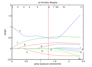
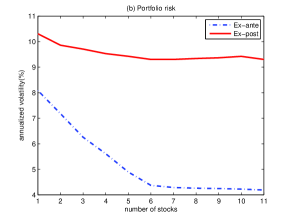
Figure 2: Illustration of risk improvement by using the constrained least-squares (3.3). On January 8, 2005, it is intended to improve the risk of the CRSP index using 10 industrial portfolios constructed by Kenneth French, using the past year daily data. (a) The solution paths for different gross exposure parameter $d$, using sample covariance matrix. The numbers on the top of the figure shows the number of assets recruited for a given $d$. (b) The ex-ante and ex-post risks (annualized volatility) of the selected portfolio. Ex-post risk is computed based on the daily returns of the selected portfolio from January 8, 2005 to January 8, 2006. They have the same decreasing pattern until 6 stocks are added.

As an illustration of the portfolio improvement, we use the daily returns of 10 industrial portfolios from the website of Kenneth French from July 1, 1963 to December 31, 2007. These portfolios are “Consumer Non-durables”, “Consumer Durables”, “Manufacturing”, “Energy”, “Hi-tech equipment”, “Telecommunication”, “Shops”, “Health”, “Utilities”, and “Others”. They are labeled, respectively, as 1 through 10 in Figure 2(a). Suppose that today is January 8, 2005, which was picked at random, and the portfolio to be improved is the CRSP value-weighted index. We wish to add some of these 10 industrial portfolios to reduce the risk of the index. Based on the sample covariance matrix, computed from the daily data between January 9, 2004 and January 8, 2005, we solve problem (3.3) based on the LARS-LASSO algorithm. The solution path $\mbox{\bf w}^{*}_{opt}(d)$ is shown in Figure 2(a). For each given $d$, the non-vanishing weights of 10 industrial portfolios are plotted along with the weight on the CRSP. They add up to one for each given $d$. For example, when $d=0$, the weight on CRSP is 1. As soon as $d$ moves slightly away from zero, the “Consumer Non-durables” (labeled as 1) are added to the portfolio, while the weight on CRSP is reduced by the same amount until at the point $d=0.23$, at which the portfolio “Utilities” (labeled as 9) is recruited. At any given $d$, the weights add up to one. Figure 2(b) gives the empirical (ex-ante) risk of the portfolio with the allocation vector $\mbox{\bf w}^{*}_{opt}(d)$ on the 10 industrial portfolios and the rest on the index. This is available for us at the time to make a decision on whether or not to modify the portfolio weights. The figure suggests that the empirical risk stops decreasing significantly as soon as the number of assets is more than 6, corresponding to $d=1.3$, shown as the vertical line in Figure 2(a). In other words, we would expect that the portfolio risk can be improved by adding selected industrial portfolios until that point. The ex-post risks based on daily returns until January 8, 2006 (one year) for these selected portfolios are also shown in Figure 2(b). As expected, the ex-post risks are much higher than the ex-ante risks. A nice surprise is that the ex-post risks also decrease until the number of selected portfolio is 6, which is in line with our decision based on the ex-ante risks. Investors can make a sensible investment decision based on the portfolio weights in Figure 2(a) and the empirical risks in Figure 2(b).

The gaps between the ex-ante and ex-post risks widen as $d$ increases. This is expected as Theorem 1 shows that the difference increases in the order of $c^{2}$, which is related to $d$ by (3.4) below. In particular, it shows that the Markowitz portfolio has the widest gap.

3.3 Approximate solution paths to risk minimization

The solution path to (3.3) also provides a nearly optimal solution path to the problem (2.6). For example, the allocation with $\mbox{\bf w}_{opt}^{*}(d)$ on the first $p-1$ stocks and the rest on the last stock is a feasible allocation vector to the problem (2.6) with

$$c=d+|1-\mbox{\bf 1}^{T}\mbox{\bf w}_{opt}^{*}(d)|.$$ (3.4)

This will not be the optimal solution to the problem (2.6) as it depends on the choice of $Y$. However, when $Y$ is properly chosen, the solution is nearly optimal, as to be demonstrated. For example, by taking $Y$ to be the no-short-sale portfolio, then problem (3.3) with $d=0$ is the same as the solution to problem (2.6) with $c=1$. We can then use (3.3) to provide a nearly optimal solution to the gross-exposure constrained risk optimization problem with $c$ given by (3.4).

In summary, to compute (2.6) for all $c$, we first find the solution with $c=1$ using a quadratic programming. This yields the optimal no-short-sale portfolio. We then take this portfolio as $Y$ in problem (3.3) and apply the LARS-LASSO algorithm to obtain the solution path $\mbox{\bf w}_{opt}^{*}(d)$. Finally, use (3.4) to convert $d$ into $c$, namely, regard the portfolio with $\mbox{\bf w}_{opt}^{*}(d)$ on the first $p-1$ stocks and the rest on the optimal no-short-sale portfolio as an approximate solution to the problem (2.6) with $c$ given by (3.4). This yields the whole solution path to the problem (2.6). As shown in Figure 3(a) below and the empirical studies, the approximation is indeed quite accurate.

In the above algorithm, one can also take a tradable index or an ETF in the set of stocks under consideration as the $Y$ variable and applies the same technique to obtain a nearly optimal solution. We have experimented this and obtained good approximations, too.

3.4 Empirical risk minimization

First of all, the constrained risk minimization problem (3.3) depends only on the covariance matrix. If the covariance matrix is given, then the solution can be found through the LARS-LASSO algorithm in Appendix B. However, if the empirical data $\{(\mbox{\bf X}_{t},Y_{t})_{t=1}^{n}\}$ are given, one naturally minimizes its empirical counterpart:

$$\min_{b,\|\mbox{\bf w}^{*}\|_{1}\leq d}\sum_{t=1}^{n}(Y_{t}-\mbox{\bf w}^{*}{}^{T}\mbox{\bf X}_{t}-b)^{2}.$$ (3.5)

Note that by using the connections in §3.1, the constrained least-squares problem (3.5) is equivalent to problem (3.3) with the population covariance matrix replaced by the sample covariance matrix: No details of the original data are needed and the LARS-LASSO algorithm in Appendix B applies.

4 Simulation studies

In this section, we use simulation studies, in which we know the true covariance matrix and hence the actual and theoretical risks, to verify our theoretical results and to quantify the finite sample behaviors. In particular, we would like to demonstrate that the risk profile of the optimal no-short-sale portfolio can be improved substantially and that the LARS algorithm yields a good approximate solution to the risk minimization with gross-exposure constraint. In addition, we would like to demonstrate that when covariance matrix is estimated with reasonable accuracy, the risk that we want and the risk that we get are approximately the same for a wide range of the exposure coefficient. When the sample covariance matrix is used, however, the risk that we get can be very different from the risk that we want for the unconstrained Markowitz mean-variance portfolio.

Throughout this paper, the risk is referring to the standard deviation of a portfolio, the square-roots of the quantities presented in Theorem 1. To avoid ambiguity, we call $\sqrt{R(\mbox{\bf w}_{opt})}$ the theoretical optimal risk or oracle risk, $\sqrt{R_{n}(\hat{\mbox{\bf w}}_{opt})}$ the empirical optimal risk, and $\sqrt{R(\hat{\mbox{\bf w}}_{opt})}$ the actual risk of the empirically optimally allocated portfolio. They are also referred to as the oracle, empirical, and actual risks.

4.1 A simulated Fama-French three-factor model

Let $R_{i}$ be the excessive return over the risk free interest rate. Fama and French (1993) identified three key factors that capture the cross-sectional risk in the US equity market. The first factor is the excess return of the proxy of the market portfolio, which is the value-weighted return on all NYSE, AMEX and NASDAQ stocks (from CRSP) minus the one-month Treasury bill rate. The other two factors are constructed using six value-weighted portfolios formed by size and book-to-market. They are the difference of returns between large and small capitalization, which captures the size effect, and the difference of returns between high and low book-to-market ratios, which reflects the valuation effect. More specifically, we assume that the excess return follows the following three-factor model:

$$R_{i}=b_{i1}f_{1}+b_{i2}f_{2}+b_{i3}f_{3}+\varepsilon_{i},\quad i=1,\cdots,p,$$ (4.1)

where $\{b_{ij}\}$ are the factor loadings of the $i^{th}$ stock on the factor $f_{j}$, and $\varepsilon_{i}$ is the idiosyncratic noise, independent of the three factors. We assume further that the idiosyncratic noises are independent of each other, whose marginal distributions are the Student-$t$ with degree of freedom 6 and standard deviation $\sigma_{i}$.

To facilitate the presentation, we write the factor model (4.1) in the matrix form:

$$\mbox{\bf R}=\mbox{\bf B}\mbox{\bf f}+\mbox{\boldmath$\varepsilon$},$$ (4.2)

where B is the matrix, consisting of the factor loading coefficients. Throughout this simulation, we assume that $E(\mbox{\boldmath$\varepsilon$}|\mbox{\bf f})=\mbox{\bf 0}$ and $\mathrm{cov}(\mbox{\boldmath$\varepsilon$}|\mbox{\bf f})=\mathrm{diag}(\sigma_{1}^{2},\cdots,\sigma_{p}^{2})$. Then, the covariance matrix of the factor model is given by

$$\mathbf{\Sigma}=\mathrm{cov}(\mbox{\bf B}\mbox{\bf f})+\mathrm{cov}(\mbox{\boldmath$\varepsilon$})=\mbox{\bf B}\mathrm{cov}(\mbox{\bf f})\mbox{\bf B}^{T}+\mbox{diag}(\sigma_{1}^{2},\cdots,\sigma_{p}^{2}).$$ (4.3)

We simulate the $n$-period returns of $p$ stocks as follows. See Fan et al.(2008) for additional details. First of all, the factor loadings are generated from the trivariate normal distribution $N(\mbox{\boldmath$\mu$}_{b},\mbox{\bf cov}_{b})$, where the parameters are given in Table 1 below. Once the factor loadings are generated, they are taken as the parameters and thus kept fixed throughout simulations. The levels of idiosyncratic noises are generated from a gamma distribution with shape parameter 3.3586 and the scale parameter 0.1876, conditioned on the noise level of at least 0.1950. Again, the realizations are taken as $p$ parameters $\{\sigma_{i}\}$ and kept fixed across simulations. The returns of the three factors over $n$ periods are drawn from the trivariate normal distribution $N(\mbox{\boldmath$\mu$}_{f},\mbox{\bf cov}_{f})$, with the parameters given in Table 1 below. They differ from simulations to simulations and are always drawn from the trivariate normal distribution. Finally, the idiosyncratic noises are generated from the Student’s t-distribution with degree of freedom 6 whose standard deviations are equal to the noise level $\{\sigma_{i}\}$. Note that both the factor returns and idiosyncratic noises change across different time periods and different simulations.

Table 1: Parameters used in the simulation

This table shows the expected values and covariance matrices for the factor loadings (left panel) and factor returns (right panel). They are used to generate factor loading parameters and the factor returns over different time periods. They were calibrated to the market.

Parameters for factor loadings					Parameters for factor returns
$\mbox{\boldmath$\mu$}_{b}$	$\mbox{\bf cov}_{b}$				$\mbox{\boldmath$\mu$}_{f}$	$\mbox{\bf cov}_{f}$
0.7828	0.02914	0.02387	0.010184		0.02355	1.2507	-0.0350	-0.2042
0.5180	0.02387	0.05395	-0.006967		0.01298	-0.0350	0.3156	-0.0023
0.4100	0.01018	-0.00696	0.086856		0.02071	-0.2042	-0.0023	0.1930

The parameters used in the simulation model (2.1) are calibrated to the market data from May 1, 2002 to August 29, 2005, which are depicted in Table 1 and taken from Fan et al.(2008) who followed closely the instructions on the website of Kenneth French, using the three-year daily return data of 30 industrial portfolios. The expected returns and covariance matrix of the three factors are depicted in Table 1. They fitted the data to the Fama-French model and obtained 30 factor loadings. These factor loadings have the sample mean vector $\mbox{\boldmath$\mu$}_{b}$ and sample covariance $\mbox{\bf cov}_{f}$, which are given in Table 1. The 30 idiosyncratic noise levels were used to determine the parameters in the Gamma distribution.

4.2 LARS approximation and portfolio improvement

Quadratic programming algorithms to problem (2.6) is relatively slow when the whole solution path is needed. As mentioned in §3.3, the LARS algorithm provides an approximate solution to this problem via (3.4). The LARS algorithm is designed to compute the whole solution path and hence is very fast. The first question is then the accuracy of the approximation. As a byproduct, we also demonstrate that the optimal no-short-sale portfolio is not diversified enough and can be significantly improved.

To demonstrate this, we took 100 stocks with covariance matrix given by (4.3). For each given $c$ in the interval $[1,3]$, we applied a quadratic programming algorithm to solve problem (2.6) and obtained its associated minimum portfolio risk. This is depicted in Figure 3(a). We also employed the LARS algorithm using the optimal no-short-sale portfolio as $Y$, with $d$ ranging from 0 to 3. This yields a solution path along with its associated portfolio risk path. Through the relation (3.4), we obtained an approximate solution to problem (2.6) and its associated risk which is also summarized in Figure 4(a). The number of stocks for the optimal no-short-sale portfolio is 9. As $c$ increases, the number of stocks picked by (2.6) also increases, as demonstrated in Figure 3(b) and the portfolio gets more diversified.

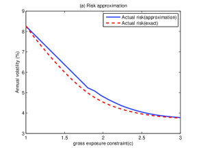
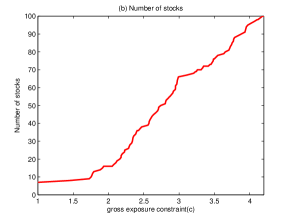
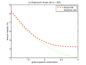
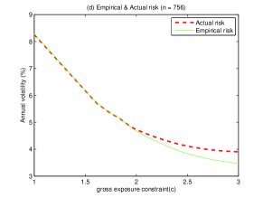
Figure 3: Comparisons of optimal portfolios selected by the exact and approximate algorithms with a known covariance matrix. (a) The risks for the exact algorithm (dashed line) and the LARS (approximate) algorithm. (b) The number of stocks picked by the optimization problem (2.6) as a function of the gross exposure coefficient $c$. (c) The actual risk (dashed line) and empirical risk (solid) of the portfolio selected based on the sample covariance matrix ($n=252$). (d) The same as (c) except $n=756$.

The approximated and exact solutions have very similar risk functions. Figure 3 showed that the optimal no-short-sale portfolio is very conservative and can be improved dramatically as the constraint relaxes. At $c=2$ (corresponding to 18 stocks with 50% short positions and 150% long positions), the risk decreases from 8.1% to 4.9%. The decrease of risks slows down dramatically after that point. This shows that the optimal no-short-sale constraint portfolio can be improved substantially by using our methods.

The next question is whether the improvement can be realized with the covariance matrix being estimated from the empirical data. To illustrate this, we simulated $n=252$ from the three-factor model (4.1) and estimated the covariance matrix by the sample covariance matrix. The actual and empirical risks of the selected portfolio for a typical simulated data set are depicted in Figure 3(c). For a range up to $c=1.7$, they are approximately the same. The range widens when the covariance matrix is estimated with a better accuracy. To demonstrate this effect, we show in Figure 3(d) the case with sample size $n=756$. However, when the gross exposure parameter is large and the portfolio is close to the Markowitz’s one, they differ substantially. See also Figure 1. The actual risk is much larger than the empirical one, and even far larger than the theoretical optimal one. Using the empirical risk as our decision guide, we can see that the optimal no-short-sale portfolio can be improved substantially for a range of the gross exposure parameter $c$.

To demonstrate further how much our method can be used to improve the existing portfolio, we assume that the current portfolio is an equally weighted portfolio among 200 stocks. This is the portfolio $Y$. The returns of these 200 stocks are simulated from model (4.1) over a period of $n=252$. The theoretical risk of this equally weighted portfolio is 13.58%, while the empirical risk of this portfolio is 13.50% for a typical realization. Here, the typical sample is referring to the one that has the median value of the empirical risks among 200 simulations. This particular simulated data set is used for the further analysis.

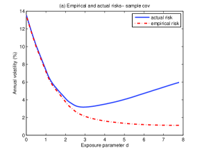
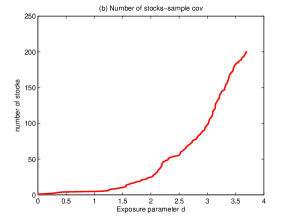
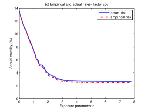
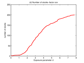
Figure 4: This is on the portfolio improvement of the 200 equally weighted portfolio by modifying the weights of the portfolio using (3.3). As the exposure parameter $d$ increases, more weights are modified and the risks of new portfolios decrease. (a) The empirical and actual risks of the modified portfolios are plotted against exposure parameter $d$, based on the sample covariance matrix. (b) The number of stocks whose weights are modified as a function of $d$. (c) and (d) are the same as (a) and (b) except that the covariance matrix is estimated based on the factor model.

We now pretend that this equally weighted portfolio is the one that an investor holds and the investor seeks possible improvement of the efficiency by modifying some of the weights. The investor employs the LARS-LASSO technique (3.3), taking the equally weighted portfolio as $Y$ and the 200 stocks as potential $X$. Figure 4 depicts the empirical and actual risks, and the number of stocks whose weights are modified in order to improve the risk profile of equally weighted portfolio.

The risk profile of the equally weighted portfolio can be improved substantially. When the sample covariance is used, at $d=1$, Figure 2(a) reveals the empirical risk is only about one half of the equally weighted portfolio, while Figure 2(b) or Table 2 shows that the number of stocks whose weights have been modified is only 4. As $d=1$, by (3.4), $c\leq 2d+1\leq 3$, which is a crude upper bound. In other words, there are at most 100% short positions. Indeed, the total percentage of short positions is only about 48%. The actual risk of this portfolio is very close to the empirical one, giving an actual risk reduction of nearly 50%. At $d=2$, corresponding to about 130% of short positions, the empirical risk is reduced by a factor of about 5, whereas the actual risk is reduced by a factor of about 4. Increasing the gross exposure parameter only slightly reduces the empirical risk, but quickly increases the actual risk. Applying our criterion to the empirical risk, which is known at the time of decision making, one would have chosen a gross exposure parameter somewhat less than 1.5, realizing a sizable risk reduction. Table 2 summarizes the actual risk, empirical risk, and the number of modified stocks under different exposure parameter $d$. Beyond $d=2$, there is very little risk reduction. At $d=5$, the weights of 158 stocks need to be modified, resulting in 250% of short positions. Yet, the actual risk is about the same as that with $d=2$.

Table 2: Empirical and actual risks for selected portfolios

This table is based on a typical simulated 252 daily returns of 200 stocks from the Fama-French three-factor model. The aim is to improve the risk of the equally weighted portfolio by modifying some of its weights. The covariance is estimated by either sample covariance (left panel) or the factor model (right panel). The penalized least-squares (3.3) is used to construct the portfolio. Reported are actual risk, empirical risk, the number of stocks whose weights are modified by the penalized least square (3.3), and percent of short positions, as a function of the exposure parameter $d$.

	Sample Covariance					Factor-model based covariance
d	Actual	Empirical	# stocks	Short		Actual	Empirical	# stocks	Short
0	13.58	13.50	0	0%		13.58	12.34	0	0%
1	7.35	7.18	4	48%		7.67	7.18	4	78%
2	4.27	3.86	28	130%		4.21	4.00	2	133%
3	3.18	2.15	84	156%		2.86	2.67	98	151%
4	3.50	1.61	132	195%		2.71	2.54	200	167%
5	3.98	1.36	158	250%		2.71	2.54	200	167%

Similar conclusions can be made for the covariance matrix based on the factor model. In this case, the covariance matrix is estimated more accurately and hence the empirical and actual risks are closer for a wider range of the gross exposure parameter $d$. This is consistent with our theory. The substantial gain in this case is due to the fact that the factor model is correct and hence incurs no modeling biases in estimating covariance matrices. For the real financial data, however, the accuracy of the factor model is unknown. As soon as $d\geq 3$ the empirical reduction of risk is not significant. The range of risk approximation is wider than that based on the sample covariance, because the factor-model based estimation is more accurate.

Figure 4(a) also supports our theory that when $c$ is large, the estimation errors of covariance matrix start to play a role. In particular, when $d=7$, which is close to the Markowitz portfolio, the difference between actual and empirical risks is substantial.

4.3 Risk approximations

We now use simulations to demonstrate the closeness of the risk approximations with the gross-exposure constraints. The simulated factor model (4.1) is used to generate the returns of $p$ stocks over a period of $n=252$ days. The number of simulations is 101. The covariance matrix is estimated by either the sample covariance or the factor model (4.3) whose coefficients are estimated from the sample. We examined two cases: $p=200$ and $p=500$. In the first case, the portfolio size is smaller than the sample size, whereas in the second the portfolio size is larger. The former corresponds to a non-degenerate sample covariance matrix whereas the latter corresponds to a degenerate one. The LARS algorithm is used to find an approximately optimal solution to problem (2.6) as it is much faster for the simulation purpose. We take $Y$ as the optimal portfolio with no-short-sale constraint.

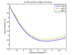
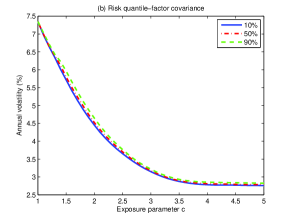
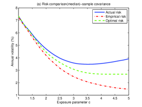
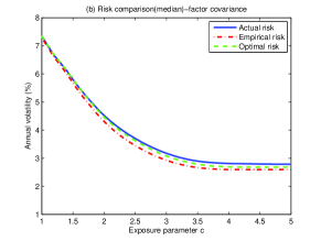
Figure 5: The 10%, 50% and 90% quantiles of the actual risks of the 101 empirically chosen portfolios for each given gross exposure parameter $c$ are shown in (a) (sample covariance matrix) and (b) (factor model) for the case with 200 stocks and the daily returns in a year. They indicate the sampling variability among 101 simulations. The theoretical optimal risk, the median of the actual risks and the median of the empirical risks of 101 empirically selected portfolios are also summarized in (c) (based on the sample covariance) and (d) (based on the factor model).

We first examine the case $p=200$ with a sample of size 252. Figure 5(a) summarizes the 10th, 50th and 90th percentiles of the actual risks of empirically selected portfolios among 101 simulations. They summarize the distributions of the actual risk of the optimally selected portfolios based on 101 empirically simulated data sets. The variations are actually small. Table 3 (bottom panel) also includes the theoretical optimal risk, the median of the actual risks of 101 empirically selected optimal portfolios, and the median of the empirical risks of those 101 selected portfolios. This part indicates the typical error of the risk approximations. It is clear from Figure 5(c) that the theoretical risk fails to decrease noticeably when $c=3$ and increasing the gross-exposure constraint will not improve very much the theoretical optimal risk profile. On the other hand, increasing gross exposure $c$ makes it harder to estimate theoretical allocation vector. As a result, the actual risk increases when $c$ gets larger.

Combining the results in both top and bottom panels, Table 3 gives a comprehensive overview of the risk approximations. For example, when the global exposure parameter is large, the approximation errors dominate the sampling variability. It is clear that the risk approximations are much more accurate for the covariance matrix estimation based on the factor model. This is somewhat expected as the data generating process is a factor model: there are no modeling biases in estimating the covariance matrix. For the sample covariance estimation, the accuracy is fairly reasonable until the gross exposure parameter exceeds 2.

Table 3: Empirical and actual risks for selected portfolios

This table is based on 101 simulations. Each simulation generates 252 daily returns of 200 stocks from the Fama-French three-factor model. The covariance is estimated by sample covariance matrix or the factor model (4.3). The penalized least-squares (3.3) is used to construct the optimal portfolios.

Sample covariance matrix
		Theorectical Cov		Sample covariance
c		Theoretical opt.		min	$1^{st}$ quantile		median	$3^{rd}$ quantile	max
1	Actual	7.35		7.35	7.36		7.37	7.38	7.43
	Empirical	7.35		6.64	7.07		7.28	7.52	8.09
2	Actual	4.46		4.48	4.64		4.72	4.78	5.07
	Empirical	4.46		3.71	4.04		4.19	4.36	4.64
3	Actual	3.07		3.41	3.53		3.58	3.66	3.84
	Empirical	3.07		2.07	2.40		2.49	2.60	2.84
4	Actual	2.69		3.31	3.47		3.54	3.61	3.85
	Empirical	2.69		1.48	1.71		1.79	1.87	2.05
5	Actual	2.68		3.62	3.81		3.92	3.99	4.25
	Empirical	2.68		1.15	1.41		1.48	1.57	1.73
Factor-based covariance matrix
1	Actual	7.35		7.35	7.36		7.37	7.39	7.41
	Empirical	7.35		6.60	7.07		7.29	7.50	8.07
2	Actual	4.46		4.46	4.48		4.52	4.57	4.74
	Empirical	4.46		3.96	4.19		4.31	4.45	4.80
3	Actual	3.07		3.14	3.16		3.18	3.19	3.26
	Empirical	3.07		2.75	2.86		2.93	2.98	3.18
4	Actual	2.69		2.76	2.79		2.81	2.83	2.90
	Empirical	2.69		2.49	2.56		2.60	2.63	2.75
5	Actual	2.68		2.73	2.77		2.78	2.80	2.87
	Empirical	2.68		2.49	2.56		2.59	2.62	2.74

Table 3 furnishes some additional details for Figure 5. For the optimal portfolios with no-short-sale constraint, the theoretical and empirical risks are very close to each other. For the global minimum variance portfolio, which corresponds to a large $c$, the empirical and actual risks of an empirically selected portfolio can be quite different. The allocation vectors based on a known covariance matrix can also be very different from that based on the sample covariance. To help gauge the scale, we note that for the true covariance, the global minimum variance portfolio has $c=4.22$, which involves 161% of short positions, and minimum risk 2.68%.

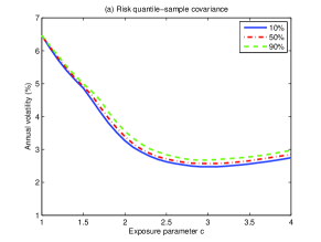
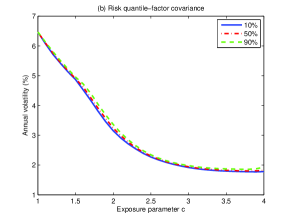
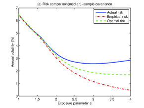
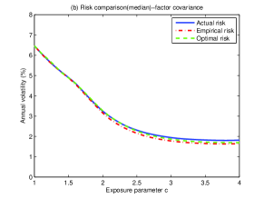
Figure 6: This is similar to Figure 5 except $p=500$. The sample covariance matrix is always degenerate under this setting ($n=252$). Nevertheless, for the given range of $c$, the gross-constrained portfolio performs normally. The same captions as Figure 5 are used.

Table 4: Empirical and actual risks for selected portfolios

This is a similar to Table 3 except $p=500$. In this case, the sample covariance matrix is always degenerate.

Sample covariance matrix
		Theoretical Cov		Sample covariance
c		Theoretical opt.		min	$1^{st}$ quantile		median	$3^{rd}$ quantile	max
1	Actual	6.47		6.47	6.48		6.49	6.50	6.53
	Empirical	6.47		5.80	6.28		6.45	6.67	7.13
2	Actual	3.27		3.21	3.29		3.39	3.47	3.73
	Empirical	3.27		2.54	2.92		3.06	3.22	3.42
3	Actual	1.87		2.42	2.53		2.57	2.63	2.81
	Empirical	1.87		0.88	1.09		1.15	1.24	1.49
4	Actual	1.69		2.65	2.79		2.85	2.92	3.21
	Empirical	1.69		0.24	0.41		0.46	0.52	0.77
Factor-based covariance matrix
1	Actual	6.47		6.47	6.48		6.49	6.51	6.55
	Empirical	6.47		5.80	6.29		6.45	6.67	7.15
2	Actual	3.27		3.16	3.21		3.35	3.39	3.48
	Empirical	3.27		2.74	3.02		3.16	3.29	3.52
3	Actual	1.87		1.91	1.93		1.94	1.96	2.02
	Empirical	1.87		1.70	1.75		1.78	1.81	1.89
4	Actual	1.69		1.75	1.79		1.82	1.85	2.87
	Empirical	1.69		1.59	1.63		1.64	1.67	2.75

We now consider the case where there are 500 potential stocks with only a year of data ($n=252$). In this case, the sample covariance matrix is always degenerate. Therefore, the global minimum portfolio based on empirical data is meaningless, which always has empirical risk zero. In other words, the difference between the actual and empirical risks of such an empirically constructed global minimum portfolio is substantial. On the other hand, with the gross-exposure constraint, the actual and empirical risks approximate quite well for a wide range of gross exposure parameters. To gauge the relative scale of the range, we note that for the given theoretical covariance, the global minimum portfolio has $c=4.01$, which involves 150% of short positions with the minimal risk 1.69%.

The sampling variability for the case with 500 stocks is smaller than the case that involves 200 stocks, as demonstrated in Figures 5 and 6. The approximation errors are also smaller. These are due to the fact that with more stocks, the selected portfolio is generally more diversified and hence the risks are generally smaller. The optimal no-short-sale portfolio, selected from 500 stocks, has actual risk 6.47%, which is not much smaller than 7.35% selected from 200 stocks. As expected, the factor-based model has a better estimation accuracy than that based on the sample covariance.

5 Empirical Studies

5.1 Fama-French 100 Portfolios

Table 5: Returns and Risks based on 100 Fama-French Industrial

We use the daily returns of 100 industrial portfolios formed by size and book to market from the website of Kenneth French from Jan 2, 1998 to December 31, 2007. At the end of each month from 1998 to 2007, the covariance of the 100 assets is estimated according to various estimators using the past 12 months’ daily return data. We use these covariance matrices to construct optimal portfolios with various exposure constraints. We hold the portfolios for one month. The means, standard deviations and other characteristics of these portfolios are recorded. (NS: no short sales portfolio; GMV: Global minimum variance portfolio)

	Mean	Std Dev	Sharpe	Max	Min	No. of Long	No. of Short
Methods	%	%	Ratio	Weight	Weight	Positions	Positions
Sample Covariance Matrix Estimator
No short(c = 1)	19.51	10.14	1.60	0.27	-0.00	6	0
Exact(c = 1.5)	21.04	8.41	2.11	0.25	-0.07	9	6
Exact(c = 2)	20.55	7.56	2.28	0.24	-0.09	15	12
Exact(c = 3)	18.26	7.13	2.09	0.24	-0.11	27	25
Approx. (c = 2, Y=NS)	21.16	7.89	2.26	0.32	-0.08	9	13
Approx. (c = 3, Y=NS)	19.28	7.08	2.25	0.28	-0.11	23	24
GMV Portfolio	17.55	7.82	1.82	0.66	-0.32	52	48
Factor-Based Covariance Matrix Estimator
No short(c = 1)	20.40	10.19	1.67	0.21	-0.00	7	0
Exact(c = 1.5)	22.05	8.56	2.19	0.19	-0.05	11	8
Exact(c = 2)	21.11	7.96	2.23	0.18	-0.05	17	18
Exact(c = 3)	19.95	7.77	2.14	0.17	-0.05	35	41
Approx. (c=2, Y=NS)	21.71	8.07	2.28	0.24	-0.04	10	19
Approx. (c=3, Y=NS)	20.12	7.84	2.14	0.18	-0.05	33	43
GMV Portfolio	19.90	7.93	2.09	0.43	-0.14	45	55
Covariance Estimation from Risk Metrics
No short(c = 1)	15.45	9.27	1.31	0.30	-0.00	6	0
Exact(c = 1.5)	15.96	7.81	1.61	0.29	-0.07	9	5
Exact(c = 2)	14.99	7.38	1.58	0.29	-0.10	13	9
Exact(c = 3)	14.03	7.34	1.46	0.29	-0.13	21	18
Approx. (c=2, Y=NS)	15.56	7.33	1.67	0.34	-0.08	9	11
Approx. (c=3, Y=NS)	15.73	6.95	1.78	0.30	-0.11	20	20
GMV Portfolio	13.99	9.47	1.12	0.78	-0.54	53	47
Unmanaged Index
Equal weighted	10.86	16.33	0.46	0.01	0.01	100	0
CRSP	8.2	17.9	0.26

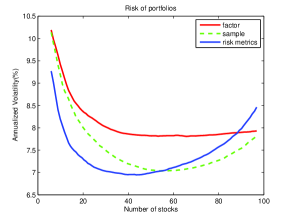
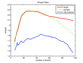
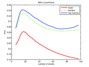
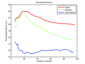
Figure 7: Characteristics of invested portfolios as a function of number of assets from the Fama-French 100 industrial portfolios formed by the size and book to market from Jan 2, 1998 to December 31, 2007. (a) Annualized risk of portfolios. (b)Sharpe ratio of portfolios. (c)Max weight of allocations. (d)Annualized return of portfolios

We use the daily returns of 100 industrial portfolios formed on size and book to market ratio from the website of Kenneth French from Jan 2, 1998 to December 31, 2007. These 100 portfolios are formed by the two-way sort of the stocks in the CRSP database, according to the market equity and the ratio of book equity to market equity, 10 categories in each variable. At the end of each month from 1998 to 2007, the covariance matrix of the 100 assets is estimated according to three estimators, the sample covariance, Fama-French 3-factor model, and the RiskMetrics with $\lambda=0.97$, using the past 12 months’ daily return data. These covariance matrices are then used to construct optimal portfolios under various exposure constraints. The portfolios are then held for one month and rebalanced at the beginning of the next month. The means, standard deviations and other characteristics of these portfolios are recorded and presented in Table 5. They represent the actual returns and actual risks. Figure 7, produced by using the LARS-LASSO algorithm, provides some additional details to these characteristics in terms of the number of assets held. The optimal portfolios with the gross-exposure constraints pick certain numbers of assets each month. The average numbers of assets over the study period are plotted in the x-axis.

First of all, the optimal no-short-sale portfolios, while selecting about 6 assets from 100 portfolios, are not diversified enough. Their risks can easily be improved by relaxing the gross-exposure constraint with $c=2$ that has 50% short positions and 150% long positions. This is shown in Table 5 and Figure 7(a), no matter which method is used to estimate the covariance matrix. The risk stops decreasing dramatically once the number of stocks exceeds 20. Interestingly, the Sharpe ratios peak around 20 stocks too. After that point, the Sharpe Ratio actually falls for the covariance estimation based on the sample covariance and the factor model.

The portfolios selected by using the RiskMetrics have lower risks. In comparison with the sample covariance matrix, the RiskMetrics estimates the covariance matrix using a much smaller effective time window. As a result, the biases are usually smaller than the sample covariance matrix. Since each asset is a portfolio in this study, its risk is smaller than stocks. Hence, the covariance matrix can be estimated more accurately with the RiskMetrics in this study. This explains why the resulting selected portfolios by using RiskMetrics have smaller risks. However, their associated returns tend to be smaller too. As a result, their Sharpe ratios are actually smaller. The Sharpe ratios actually peak at around 50 assets.

It is surprising to see that the unmanaged equally weighted portfolio, which invests 1 percent on each of the 100 industrial portfolios, is far from optimal in terms of the risk during the study period. The value-weighted index CRSP does not fare much better. They are all outperformed by the optimal portfolios with gross-exposure constraints during the study period. This is in line with our theory. Indeed, the equally weighted portfolio and CRSP index are two specific members of the no-short-sale portfolio, and should be outperformed by the optimal no-short-sale portfolio, if the covariance matrix is estimated with reasonable accuracy.

From Table 5, it can also be seen that our approximation algorithm yields very close solution to the exact algorithm. For example, using the sample covariance matrix, the portfolios constructed using the exact algorithm with $c=3$ has the standard deviation of 7.13%, whereas the portfolios constructed using the approximate algorithm has the standard deviation of 7.08%. In terms of the average numbers of selected stocks over the 10-year study period, they are close too.

5.2 Russell 3000 Stocks

Table 6: Returns and Risks based on random 400 portfolio

We pick 1000 stocks from Russell 3000 with least percents of missing data from Jan 2, 2003 to December 31, 2007. Among the 1000 stocks, we randomly pick 400 stocks to avoid survival bias. At the end of each month from 2003 to 2007, the covariance of the 400 stocks is estimated according to various estimators using the past 24 months’ daily return data. We use these covariance matrices to construct optimal portfolios under various gross-exposure constraints. We hold the portfolio for one month. The standard deviations and other characteristics of these portfolios are recorded. (NS: no short sales; MKT: return of S&P 500 index; GMV: Global minimum variance portfolio)

	Std Dev	Max	Min	No. of Long	No. of Short
Methods	%	Weight	Weight	Positions	Positions
Sample Covariance Matrix Estimator
No short	9.72	0.17	-0.00	51	0
Approx (NS, c= 1.5)	8.85	0.21	-0.06	54	33
Approx (NS, c= 2)	8.65	0.19	-0.07	83	62
Approx (NS, c= 2.5)	8.62	0.17	-0.08	111	84
Approx (NS, c= 3)	8.80	0.16	-0.08	131	103
Approx (NS, c= 3.5)	9.08	0.15	-0.09	149	120
Approx (MKT, c =1.5)	8.79	0.15	-0.08	61	42
Approx (MKT, c =2)	8.64	0.15	-0.08	87	66
Approx (MKT, c =2.5)	8.69	0.15	-0.09	109	88
Approx (MKT, c =3)	8.87	0.14	-0.09	128	108
Approx (MKT, c =3.5)	9.08	0.14	-0.10	143	124
GMV portfolio	14.40	0.26	-0.27	209	191
Factor-Based Covariance Matrix Estimator
No short	9.48	0.17	-0.00	51	0
Approx (NS, c= 1.5)	8.57	0.20	-0.06	54	36
Approx (NS, c= 2)	8.72	0.13	-0.05	123	94
Approx (NS, c= 2.5)	9.09	0.08	-0.05	188	159
Approx (MKT, c =1.5)	8.84	0.13	-0.06	73	43
Approx (MKT, c =2)	8.87	0.10	-0.05	126	94
Approx (MKT, c =2.5)	9.07	0.08	-0.04	189	164
GMV portfolio	9.23	0.08	-0.05	212	188
Covariance Estimation from Risk Metrics
No short	10.64	0.54	-0.00	27	0
Approx (NS, c= 1.5)	10.28	0.56	-0.05	38	25
Approx (NS, c= 2)	8.73	0.23	-0.08	65	43
Approx (NS, c= 2.5)	8.58	0.17	-0.08	94	67
Approx (NS, c= 3)	8.71	0.16	-0.09	119	90
Approx (NS, c= 3.5)	9.04	0.15	-0.10	139	107
Approx (MKT, c =1.5)	8.70	0.27	-0.15	34	29
Approx (MKT, c =2)	8.63	0.17	-0.12	60	49
Approx (MKT, c =2.5)	8.58	0.14	-0.12	89	74
Approx (MKT, c =3)	8.65	0.15	-0.12	111	97
Approx (MKT, c =3.5)	8.88	0.15	-0.13	131	114
GMV portfolio	14.67	0.27	-0.27	209	191

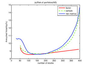
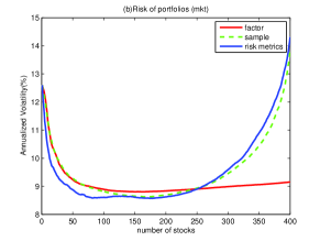
Figure 8: Risks of the optimal portfolios as a function of number of stocks for the 400 randomly selected stocks from Russell 3000. The plotted is the the annualized volatility of the optimal portfolios by taking (a) the no short-sale portfolio as $Y$ and (b) the S&P 500 stock index as $Y$. The results are very similar and demonstrate that the optimal no-short-sale portfolio is not diversified whereas the global minimum portfolio is unstable. Both portfolios can be improved by an optimal portifolio with number of stocks around 100.

We now apply our techniques to study the portfolio behavior using Russell 3000 stocks. The study period is from January 2, 2003 to December 31, 2007. To avoid computation burden and the issues of missing data, we picked 1000 stocks from 3000 stocks that constitutes Russell 3000 on December 31, 2007. Those 1000 stocks have least percents of missing data in the five-year study period. This forms the universe of the stocks under our study. To mitigate the possible survival biases, at the end of each month, we randomly selected 400 stocks from the universe of the stocks. Therefore, the 400 stocks used in one month differs substantially from those used in another month. The optimal no-short-sale portfolios, say, in one month differ also substantially from that in the next month, because they are constructed from very different pools of stocks.

At the end of each month from 2003 to 2007, the covariance of the 400 stocks is estimated according to various estimators using the past 24 months’ daily returns. Since individual stocks have higher volatility than individual portfolios, the longer time horizon than that in the study of the 100 Fama-French portfolios is used. We use these covariance matrices to construct optimal portfolios under various gross-exposure constraints and hold these portfolios for one month. The daily returns of these portfolios are recorded and hence the standard deviations are computed. We did not compute the mean returns, as the universes of stocks to be selected from differ substantially from one month to another, making the returns of the portfolios change substantially from one month to another. Hence, the aggregated returns are less meaningful than the risk.

Table 6 summarizes the risks of the optimal portfolios constructed using 3 different methods of estimating covariance matrix and using 6 different gross-exposure constraints. As the number of stocks involved is 400, the quadratic programming package that we used can fail to find the exact solution to problem (2.6). It has too many variables for the package to work properly. Instead, we computed only approximate solutions taking two different portfolios as the $Y$ variable.

The global minimum portfolio is not efficient for vast portfolios due to accumulation of errors in the estimated covariance matrix. This can be seen easily from Figure 8. The ex-post annualized volatilities of constructed portfolios using the sample covariance and RiskMetrics shoot up quickly (after 200 stocks chosen) as we increase the number of stocks (or relax the gross-exposure constraint) in our portfolio. The risk continues to grow if we relax further the gross-exposure constraint, which is beyond the range of our pictures. The maximum and minimum weights are very extreme for the global minimum portfolio when the sample covariance matrix and the RiskMetrics are used. This is mainly due to the errors in these estimated covariance matrices. The problem is mitigated when the gross-exposure constraints are imposed.

The optimal no-short-sale portfolios are not efficient in terms of ex-post risk calculation. They can be improved, when portfolios are allowed to have 50% short positions, say, corresponding to $c=2$. This is due to the fact that the no-short-sale portfolios are not diversified enough. The risk approximations are accurate beyond the range of $c=1$. On the other hand, the optimal no-short-sale portfolios outperform substantially the global minimum portfolios, which is consistent with the conclusion drawn in Jagannathan and Ma (2003) and with our risk approximation theory. When the gross-exposure constraint is loose, the risk approximation is not accurate and hence the empirical risk is overly optimistic. As a result, the allocation vector that we want from the true covariance matrix is very different from the allocation vector that we get from the empirical data. As a result, the actual risk can be quite far away from the true optimal.

The risks of optimal portfolios tend to be smaller and stable, when the covariance matrix is estimated from the factor model. For vast portfolios, such an estimation of covariance matrix tends to be most stable among the three methods that we considered here. As a result, its associated portfolio risks tend to be the smallest among the three methods. As the covariance matrix estimated by using RiskMetrics uses a shorter time window than that based on the sample covariance matrix, the resulting estimates tend to be even more unstable. As a result, its associated optimal portfolios tend to have the highest risks.

The results that we obtain by using two different approximate methods are actually very comparable. This again provides an evidence that the approximate algorithm yields the solutions that are close to the exact solution.

6 Conclusion

The portfolio optimization with the gross-exposure constraint bridges the gap between the optimal no-short-sale portfolio studied by Jagannathan and Ma (2003) and no constraint on short-sale in the Markowitz’s framework. The gross-exposure constraint helps control the discrepancies between the empirical risk which is always overly optimistic, oracle risk which is not obtainable, and the actual risk of the selected portfolio which is unknown. We demonstrate that for a range of gross exposure parameters, these three risks are actually very close. The approximation errors are controlled by the worst elementwise estimation error of the vast covariance matrix. There is no accumulation of estimation errors, thanks to the constraint on the gross exposure.

We provided theoretical insights into the observation made by Jagannathan and Ma (2003) that the optimal no-short-sale portfolio has smaller actual risk than the global minimum portfolio for vast portfolios and offered empirical evidence to strengthen the conclusion. We demonstrated that the optimal no-short-sale portfolio is not diversified enough. It is still a conservative portfolio that can be improved by allowing some short positions. This is demonstrated by our empirical studies and supported by our risk approximation theory: Increasing gross exposure somewhat does not excessively increase the risk approximation errors, but increases significantly the space of allowable portfolios and hence decreases drastically the oracle risk and the actual risk.

Practical portfolio choices always involve constraints on individual assets such as the allocations are no larger than certain percentages of the median daily trading volume of an asset. This is commonly understood as an effort of reducing the risks of the selected portfolios. Our theoretical result provides further mathematical insights to support such a statement. The constraints on individual assets also put a constraint on the gross exposure and hence control the risk approximation errors, which makes the empirical risk and actual risk closer.

Our studies have also important implications in the practice of portfolio allocation. We provide a fast approximate algorithm to find the solution paths to the constrained risk minimization problem. We demonstrate that the sparsity of the portfolio selection with gross-exposure constraint. For a given covariance matrix, we were able to find the optimal number of assets, ranging from $N_{0}$ to the total number of stocks under consideration, where $N_{0}$ is number of assets in the optimal no-short-sale portfolio. This reduces an NP-complete hard optimization problem to a problem that can be solved efficiently. In addition, the empirical risks of the selected portfolios help us to select a portfolio with a small actual risk. Our methods can also be used for portfolio tracking and improvement.

Throughout this appendix, we will assume that $\mbox{\boldmath$\mu$}=E\mbox{\bf R}_{t}$ and $\mbox{\bf S}=E(\mbox{\bf R}_{t}\mbox{\bf R}_{t}^{T})$ are independent of $t$. Let ${\cal F}_{t}$ be the filtration generated by the process $\{\mbox{\bf R}_{t}\}$.

Condition 1: Let $\mbox{\bf Y}_{t}$ be the $p(p+1)/2$-dimensional vector constructed from the symmetric matrix $\mbox{\bf R}_{t}\mbox{\bf R}_{t}^{T}-\mbox{\bf S}$. Assume that $\mbox{\bf Y}_{t}$ follows the vector autoregressive model:

$$\mbox{\bf Y}_{t}=\mbox{\bf A}_{1}\mbox{\bf Y}_{t-1}+\cdots+\mbox{\bf A}_{k}\mbox{\bf Y}_{t-k}+\mbox{\boldmath$\varepsilon$}_{t},$$

for coefficient matrices $\mbox{\bf A}_{1},\cdots,\mbox{\bf A}_{k}$ with $E\{\mbox{\boldmath$\varepsilon$}_{t}|{\cal F}_{t}\}=0$ and $\max_{t}E\|\mbox{\boldmath$\varepsilon$}_{t}\|_{\infty}<\infty$. Assume in addition that $\sup_{t}E\|\mbox{\bf A}_{j}\mbox{\bf Y}_{t}\|_{\infty}=O_{p}(n^{1/2})$ for all $1\leq j\leq k$ and $\|\mbox{\bf b}_{(j)}\|_{1}<\infty$ where $\mbox{\bf b}_{(j)}$ is the $j$-th row of matrix $\mbox{\bf B}^{-1}$, with $\mbox{\bf B}=\mbox{\bf I}-\mbox{\bf A}_{1}-\cdots-\mbox{\bf A}_{k}$. In addition, we assume similar conditions hold for the return vector $\{\mbox{\bf R}_{t}\}$.

Before introducing Condition 2, let us introduce the strong mixing coefficient $\alpha(k)$ of the process $\{\mbox{\bf R}_{t}\}$, which is given by

$$\alpha(k)=\sup_{t}\sup\{|P(AB)-P(A)P(B)|:A\in\sigma(\mbox{\bf R}_{s},s\leq t),\;B\in\sigma(\mbox{\bf R}_{s},s\geq t+k)\},$$

where $\sigma(\mbox{\bf R}_{s},s\leq t)$ is the sigma-algebra generated by $\{\mbox{\bf R}_{s},s\leq t\}$.

Condition 2. Suppose that $\|\mbox{\bf R}_{t}\|_{\infty}<B$ for a constant $B>0$ and that as $q\to\infty$, $\alpha(q)=O(\exp(-Cq^{1/b}))$ and $a>(b+1)/2$ in Theorem 3. In addition, $\log n=O(\log p)$.

Condition 3. Let $\eta_{t}$ be $R_{ti}R_{tj}-ER_{ti}R_{tj}$ or $R_{ti}-ER_{ti}$ (We suppress its dependence on $i$ and $j$). Assume that for all $i$ and $j$ there exist nonnegative constants $a$, $b$, and $B$ and a function $\rho(\cdot)$ such that

$$|\mathrm{cov}(\eta_{s_{1}}\cdots\eta_{s_{u}},\eta_{t_{1}}\cdots\eta_{t_{v}})|\leq B^{u+v}[(u+v)!]^{b}v\rho(t_{1}-s_{u}),$$

for any $1\leq s_{1}\leq\cdots\leq s_{u}\leq t_{1}\leq\cdots\leq t_{v}\leq n$ where

$$\sum_{s=0}^{\infty}(s+1)^{k}\rho(s)\leq B^{k}(k!)^{a}\qquad\mbox{for all $k>0$.}$$

and

$$E|\eta_{t}|^{k}\leq(k!)^{\nu}B^{k},\qquad\mbox{for all $k>0$.}$$

In addition, we assume that $\log p=o(n^{1/(2a+2b+3)})$.

Proof of Theorem 1: First of all, $R(\hat{}\mbox{\bf w}_{opt})-R(\mbox{\bf w}_{opt})\geq 0$, since $\mbox{\bf w}_{opt}$ minimizes the function $R$. Similarly, we have $R_{n}(\hat{}\mbox{\bf w}_{opt})-R_{n}(\mbox{\bf w}_{opt})\leq 0$. Consequently, we have

$$R(\hat{}\mbox{\bf w}_{opt})-R(\mbox{\bf w}_{opt}) = R(\hat{}\mbox{\bf w}_{opt})-R_{n}(\hat{}\mbox{\bf w}_{opt})+R_{n}(\hat{}\mbox{\bf w}_{opt})-R_{n}(\mbox{\bf w}_{opt})+R_{n}(\mbox{\bf w}_{opt})-R(\mbox{\bf w}_{opt})$$ (A.1)

$$\leq R(\hat{}\mbox{\bf w}_{opt})-R_{n}(\hat{}\mbox{\bf w}_{opt})+R_{n}(\mbox{\bf w}_{opt})-R(\mbox{\bf w}_{opt})$$

$$\leq 2\mbox{sup}_{||\mbox{\bf w}||\leq c}|R_{n}(\mbox{\bf w})-R(\mbox{\bf w})|.$$

Now, it is easy to see that

$$|R_{n}(\mbox{\bf w})-R(\mbox{\bf w})|=|\mbox{\bf w}^{T}(\hat{\mbox{\boldmath$\Sigma$}}-\mbox{\boldmath$\Sigma$})\mbox{\bf w}|\leq a_{n}\|\mbox{\bf w}\|_{1}^{2},$$ (A.2)

which is bounded by $a_{n}c^{2}$. This together with (A.1) proves the first conclusion and the second conclusion.

To prove the third inequality, we note that

$$|R(\mbox{\bf w}_{opt})-R_{n}(\hat{\mbox{\bf w}}_{opt})| \leq |R(\mbox{\bf w}_{opt})-R(\hat{\mbox{\bf w}}_{opt})|+|R(\hat{}\mbox{\bf w}_{opt})-R_{n}(\hat{\mbox{\bf w}}_{opt})|$$

$$\leq 3\mbox{sup}_{||\mbox{\bf w}||\leq c}|R_{n}(\mbox{\bf w})-R(\mbox{\bf w})|$$

where we used (A.1) to bound the first term. The third inequality comes from (A.2).

We need the following lemma to prove Theorem 2.

Lemma 1. Let $\mbox{\boldmath$\xi$}_{1},\cdots,\mbox{\boldmath$\xi$}_{n}$ be a $p$-dimensional random vector. Assume that $\mbox{\boldmath$\xi$}_{t}$ is $\mathcal{F}_{t}$-adaptive and each component is a martingale difference: $E(\mbox{\boldmath$\xi$}_{t+1}|\mathcal{F}_{t})=0$. Then, for any $p\geq 3$ and $r\in[2,\infty]$, we have for some universal constant $C$

$$E||\sum_{t=1}^{n}\mbox{\boldmath$\xi$}_{t}||_{r}^{2}\leq C\>\mbox{min}[r,\log p]\sum_{t=1}^{n}E||\mbox{\boldmath$\xi$}_{t}||_{r}^{2}$$ (A.3)

where $||\mbox{\boldmath$\xi$}_{t}||_{r}$ is the $l_{r}$-norm of the vector $\mbox{\boldmath$\xi$}_{t}$ in $R^{p}$.

This is an extension of the Nemirovski’s inequality to the marginale difference sequence. The proof follows similar arguments on page 188 of Emery el al (2000).

Proof of lemma 1. Let $V(\mbox{\bf x})=||\mbox{\bf x}||_{r}^{2}$. Then, there exists a universal constant $C$ such that

$$V(\mbox{\bf x}+\mbox{\bf y})\leq V(\mbox{\bf x})+\mbox{\bf y}^{T}V^{\prime}(\mbox{\bf x})+CrV(\mbox{\bf y}),$$

where $V^{\prime}(\mbox{\bf x})$ is the gradient vector of $V(\mbox{\bf x})$. Using this, we have

$$V(\sum_{t=1}^{n}\mbox{\boldmath$\xi$}_{t})\leq V(\sum_{t=1}^{n-1}\mbox{\boldmath$\xi$}_{t})+\mbox{\boldmath$\xi$}_{n}^{T}V^{\prime}(\sum_{t=1}^{n-1}\mbox{\boldmath$\xi$}_{t})+CrV(\mbox{\boldmath$\xi$}_{n}).$$ (A.4)

Since $\mbox{\boldmath$\xi$}_{n}$ is a martingale difference and $V^{\prime}(\sum_{t=1}^{n-1}\mbox{\boldmath$\xi$}_{t})$ is $\mathcal{F}_{n-1}$ adaptive, we have

$$E\mbox{\boldmath$\xi$}_{n}^{T}V^{\prime}(\sum_{t=1}^{n-1}\mbox{\boldmath$\xi$}_{t})=0.$$

By taking the expectation on both sides of (A.4), we have

$$EV(\sum_{t=1}^{n}\mbox{\boldmath$\xi$}_{t})\leq EV(\sum_{t=1}^{n-1}\mbox{\boldmath$\xi$}_{t})+CrEV(\mbox{\boldmath$\xi$}_{n}).$$

Iteratively applying the above formula, we have

$$E\|\sum_{t=1}^{n}\mbox{\boldmath$\xi$}_{t}\|_{r}^{2}\leq Cr\sum_{t=1}^{n}\|\mbox{\boldmath$\xi$}_{t}\|_{r}^{2}.$$ (A.5)

This proves the first half of the inequality (A.3).

To prove the inequality (A.3), without loss of generality, assume that $r\geq\log p.$ Let $r^{\prime}=\log p>1$. Then, for any x in the $p$-dimensional space,

$$\|\mbox{\bf x}\|_{r}\leq\|\mbox{\bf x}\|_{r^{\prime}}\leq p^{\frac{1}{r^{\prime}}-\frac{1}{r}}||\mbox{\bf x}||_{r}$$

Hence, by (A.5)

$$E||\sum_{t=1}^{n}\xi_{t}||_{r}^{2} \leq E||\sum_{t=1}^{n}\mbox{\boldmath$\xi$}_{t}||_{r^{\prime}}^{2}$$

$$\leq C\log p\sum_{t=1}^{n}E||\mbox{\boldmath$\xi$}_{t}||_{r^{\prime}}^{2}$$

$$\leq C\log p\sum_{t=1}^{n}p^{2(\frac{1}{r^{\prime}}-\frac{1}{r})}E||\mbox{\boldmath$\xi$}_{t}||_{r}^{2}$$

Using the simple fact $p^{\frac{2}{r^{\prime}}}=e^{2}$, we complete the proof of the inequality (A.3).

Proof of Theorem 2. Applying lemma 1, with $r=\infty$, we have

$$E\|n^{-1}\sum_{t=1}^{n}\mbox{\boldmath$\xi$}_{t}\|_{\infty}^{2}\leq\frac{C\log p}{n}\max_{t}E\|\mbox{\boldmath$\xi$}_{t}\|_{\infty}^{2},$$ (A.6)

for all $t$, where $E\|\mbox{\boldmath$\xi$}_{t}\|_{\infty}^{2}=E(\max_{1\leq j\leq p}\xi_{tj}^{2})$. As a result, by Condition 1, an application of (A.6) to $p(p+1)/2$-element of $\mbox{\boldmath$\varepsilon$}_{t}$ yields

$$E\|(n-k)^{-1}\sum_{t=k+1}^{n}(\mbox{\bf Y}_{t}-\mbox{\bf A}_{1}\mbox{\bf Y}_{t-1}-\cdots-\mbox{\bf A}_{k}\mbox{\bf Y}_{t-k})\|_{\infty}^{2}\leq\frac{C\log p^{2}}{n-k}\max_{t}E\|\mbox{\boldmath$\varepsilon$}_{t}\|_{\infty}^{2}.$$

Note that each of the summation $(n-k)^{-1}\sum_{t=k+1}^{n}\mbox{\bf Y}_{t-j}$ (for $j\leq k$) is approximately the same as $n^{-1}\sum_{t=1}^{n}\mbox{\bf Y}_{t}$ since $k$ is finite, by appealing to Condition 1. Hence, we can easily show that

$$\|\mbox{\bf B}n^{-1}\sum_{t=1}^{n}\mbox{\bf Y}_{t}\|_{\infty}=O_{p}\left(\sqrt{\frac{\log p}{n}}\right).$$

By the assumption on the matrix B, we can easily deduce that

$$\|n^{-1}\sum_{t=1}^{n}\mbox{\bf Y}_{t}\|_{\infty}=O_{p}\left(\sqrt{\frac{\log p}{n}}\right).$$

Rearranging this into matrix form, we conclude that

$$\|n^{-1}\sum_{t=1}^{n}\mbox{\bf R}_{t}\mbox{\bf R}_{t}^{T}-\mbox{\bf S}\|_{\infty}=O_{p}\left(\sqrt{\frac{\log p}{n}}\right).$$

Let $\bar{\mbox{\bf R}}_{n}=n^{-1}\sum_{t=1}^{n}\mbox{\bf R}_{t}$. As $\mbox{\bf R}_{t}$ satisfies similar conditions to $\mbox{\bf Y}_{t}$, we have also that

$$\|\bar{\mbox{\bf R}}_{n}-\mbox{\boldmath$\mu$}\|_{\infty}=O_{p}\left(\sqrt{\frac{\log p}{n}}\right).$$

Finally, by using

$$\hat{\mbox{\bf S}}_{n}=n^{-1}\sum_{t=1}^{n}\mbox{\bf R}_{t}\mbox{\bf R}_{t}^{T}-\bar{\mbox{\bf R}}_{n}\bar{\mbox{\bf R}}_{n}^{T},$$

we conclude that

$$\|\hat{\mbox{\bf S}}_{n}-\mbox{\boldmath$\Sigma$}\|_{\infty}=O_{p}\left(\sqrt{\frac{\log p}{n}}\right).$$

Proof of Theorem 3. Note that by the union bound of probability, we have for any $D>0$,

$$P\{\sqrt{n}\|\mbox{\boldmath$\Sigma$}-\hat{\mbox{\boldmath$\Sigma$}}\|_{\infty}>D(\log p)^{a}\}\leq p^{2}\max_{i,j}P\{\sqrt{n}|\sigma_{ij}-\hat{\sigma}_{ij}|>D(\log p)^{a}\}.$$

By the assumption, the above probability is bounded by

$$p^{2}\exp\left(-C[D(\log p)^{a}]^{1/a}\right)=p^{2}p^{-CD^{1/a}},$$

which tends to zero when $D$ is large enough. This proves the first part of the theorem.

We now prove the second part of the $\alpha$-mixing process. Let $\xi_{t}$ be an $\mathcal{F}_{t}$ adaptive random variable with $E\xi_{t}=0$ and assume that $|\xi_{t}|\leq B$ for all $t$. Then, by Theorem 1.3 of Bosq (1998), for any integer $q\leq n/2$, we have

$$P(|\bar{\xi}_{n}|>\varepsilon)\leq 4\exp(-\frac{q\varepsilon^{2}}{8B^{2}})+22(1+4B/\varepsilon)^{1/2}q\alpha\left([n/(2q)]\right),$$ (A.7)

where $\bar{\xi}_{n}=n^{-1}\sum_{t=1}^{n}\xi_{t}$. Taking $\varepsilon_{n}=4BD(\log p)^{a}/\sqrt{n}$ and $q=n(\log p)^{1-2a}/2$, we obtain from (A.7) that

$$P(|\bar{\xi}_{n}|>\varepsilon_{n})=4p^{-D^{2}}+o(n^{3/2})\alpha((\log p)^{2a-1})$$

Now, the assumption on the mixing coefficient $\alpha(\cdot)$, we conclude that for sufficiently large $D$,

$$P(|\bar{\xi}_{n}|>\varepsilon_{n})=o(p^{-2}),$$ (A.8)

for $a>(b+1)/2$.

Applying (A.8) to $\xi_{t}=R_{ti}R_{tj}-ER_{ti}R_{tj}$ with a sufficiently large $D$, we have

$$P(n^{-1}\sum_{t=1}^{n}|R_{ti}R_{tj}-ER_{i}R_{j}|>\varepsilon_{n})=o(p^{-2}).$$

This together with the first part of proof of Theorem 2 yield that

$$\|n^{-1}\sum_{t=1}^{n}\mbox{\bf R}_{t}\mbox{\bf R}_{t}^{T}-\mbox{\bf S}\|_{\infty}=O_{p}\left(\varepsilon_{n}\right),$$

where we borrow the notation from the proof of Theorem 2. Similarly, by an application of (A.8), we obtain

$$\|\bar{\mbox{\bf R}}_{n}-\mbox{\boldmath$\mu$}\|_{\infty}=O_{p}\left(\varepsilon_{n}\right).$$

Combining the last two results, we prove the second part of the theorem.

The proof of the third part of the theorem follows similar steps. By Theorem 1 of Doukhan and Neumann (2007), under Condition 3, we have

$$P(|\sum_{t=1}^{n}\eta_{t}|>\sqrt{n}x)\leq\exp(-C\min\{x^{2},(\sqrt{n}x)^{c}\})$$

for some $C>0$, where $c=1/(a+b+2)$. Now, taking $x=D(\log p)^{1/2}$, we have

$$x^{2}/(\sqrt{n}x)^{c}=O((\log p)^{1-c/2}/n^{c/2})=o(1),$$

since $\log p=o(n^{1/(2\mu+2\nu+3)})$. Thus, the exponent is as large as

$$C\min\{x^{2},(\sqrt{n}x)^{c}\}\geq CD^{2}\log p,$$

for sufficiently large $n$. Consequently,

$$P(|\sum_{t=1}^{n}\eta_{t}|>D\sqrt{n\log p})\leq\exp(-CD^{2}\log p)=o(p^{-2})$$

for sufficiently large $D$. Now, substituting the definition of $\eta_{t}$, we have

$$P(n^{-1}\sum_{t=1}^{n}|R_{ti}R_{tj}-ER_{i}R_{j}|>D\sqrt{(\log p)/n})=o(p^{-2}).$$ (A.9)

$$P(n^{-1}\sum_{t=1}^{n}|R_{ti}-ER_{i}|>D\sqrt{(\log p)/n})=o(p^{-2}).$$ (A.10)

Combining the results in (A.9) and (A.10) and using the same argument as proving the first part of Theorem 2, we have

$$\|n^{-1}\sum_{t=1}^{n}\mbox{\bf R}_{t}\mbox{\bf R}_{t}^{T}-\mbox{\bf S}\|_{\infty}=O_{p}\left(\sqrt{(\log p)/n}\right).$$

and

$$\|n^{-1}\sum_{t=1}^{n}\mbox{\bf R}_{t}-\mbox{\boldmath$\mu$}\|_{\infty}=O_{p}\left(\sqrt{(\log p)/n}\right).$$

The conclusion follows from these two results.

Appendix B: LARS-LASSO Algorithms for Constrained Risk Minimization

We now describe the LARS-LASSO algorithm for the constrained least-square problem (3.3). First, standardize each variable $X_{j}$ so that it has unit variance. The basic idea is very intuitive. As soon as $d$ moves slightly away from zero, one picks only one variable, which has the maximum absolute correlation with the response variable $Y$. Without loss of generality, let us assume that the maximum absolute correlation achieves at the first variable and the correlation is negative. Then, $\mbox{\bf w}^{*}=(-d,0,\cdots,0)^{T}$ is the solution to problem (3.3) for some small $d$. Now, as $d$ increases, the absolution correlation of the working residual $R=Y-\mbox{\bf X}^{T}\mbox{\bf w}=Y+dX_{1}$ with $X_{1}$ decreases until a (smallest) value $d_{1}$ at which there exists a second variable $X_{2}$, say, that has the same absolution correlation with $R$. Then, w is the solution to problem (3.3) for $0\leq d\leq d_{1}$. For $d$ slightly bigger than $d_{1}$, there are two non-vanishing components in $\mbox{\bf w}_{\delta}=\mbox{\bf w}_{1}+\delta\mbox{\boldmath$\gamma$}$, where $\mbox{\bf w}_{1}=(-d_{1},0,\cdots,0)$ and the direction $\gamma$, having only first two elements non-vanishing, is chosen so that the absolute correlations of the working residual $R=Y-\mbox{\bf X}^{T}\mbox{\bf w}_{\delta}$ with $X_{1}$ and $X_{2}$ decrease equally as $\delta$ increases until a point $\delta_{1}$ at which a third variable, $X_{3}$, say, has the same absolute correlation with the working residual as those with $X_{1}$ and $X_{2}$. The solution to problem (3.3) simply $\mbox{\bf w}_{\delta}$ for $d\in(d_{1},\|\mbox{\bf w}_{\delta_{1}}\|_{1}]$. For $d$ going slightly beyond that point, the solution to problem (3.3) consists of 3 variables. Continuing this process, we will get the whole solution path.

The LARS algorithm runs as follows. Let

$$\sigma_{j}=\mathrm{cov}(X_{j},Y)\quad\mbox{and}\quad\mbox{\boldmath$\xi$}_{j}=\mathrm{cov}(X_{j},\mbox{\bf X}),$$

which are obtained from the input covariance matrix.

1. Set the initial value $\mbox{\bf w}=0$. This corresponds to the solution with $d=0$.

2. Compute $u=\max_{j}|\sigma_{j}-\mbox{\boldmath$\xi$}_{j}^{T}\mbox{\bf w}|$, which is the maximum absolute correlation (multipled by the standard deviation of $Y$) between the working residual $R=Y-\mbox{\bf X}^{T}\mbox{\bf w}$ and $X_{j}$. Let ${\cal C}$ be index of assets that achieved the maximum absolute correlation.

3. Increase the value w for the components in ${\cal C}$ in the direction $\mbox{\boldmath$\gamma$}_{{\cal C}}$ until a new variable is added to the set ${\cal C}$. The direction $\mbox{\boldmath$\gamma$}_{{\cal C}}$ is chosen so that the absolute correlations of the working residual with all variables $\{X_{j},j\in{\cal C}\}$ decrease equally. The direction $\mbox{\boldmath$\gamma$}_{{\cal C}}$ can easily be determined analytically and so is the thresholding value for the amount of the increase.

4. Repeat Steps 2 and 3 until all variables are recruited.

References

- [1] Aït-Sahalia, Y., Mykland, P. A. and Zhang, L. (2005). How often to sample a continuous-time process in the presence of market microstructure noise. Review of Financial Studies, 18, 351-416.
- [2]
- [3] Andersen, T. G., Bollerslev, T., Diebold, F. X. and Labys, P. (2003). Modeling and forecasting realized volatility. Econometrica, 71, 579-625.
- [4]
- [5] Artzner, P., Delbaen, F., Eber, J. and Heath, D. (1999). Coherent measures of risk. Mathematical Finance, 9, 203-228.
- [6]
- [7] Barndorff-Nielsen, O., Hansen, P., Lunde, A. and Shephard, N. (2008). Multivariate realised kernels. Manuscript
- [8]
- [9] Barndoff-Neilsen, O.E. and Shephard, N. (2002). Econometric analysis of realized volatility and its use in estimating stochastic volatility models. Jour. Roy. Statist. Soc. B, 64, 253-280.
- [10]
- [11] Best, M.J. and Grauer, R.R. (1991). On the sensitivity of mean-variance-efficient portfolios to changes in asset means: Some analytical and computational results. Review of Financial Studies, 2, 315-342.
- [12]
- [13] Black, F. (1972). Capital market equilibrium with restricted borrowing. Journal of Business, 45, 444-454.
- [14]
- [15] Brodie, et al. 2008, Sparse and stable Markowitz portfolios. CEPR Discussion Paper No. DP6474
- [16]
- [17] Bosq, D. (1998). Nonparametric Statistics for Stochastic Processes: Estimation and Prediction (2nd ed.). Lecture Notes in Statistics, 110. Springer-Verlag, Berlin.
- [18]
- [19] Chopra, V.K. and Ziemba, W.T. (1993). The effect of errors in means, variance and covariances on optimal portfolio choice. Journal of Portfolio Management, winter, 6-11.
- [20]
- [21] De Roon, F. A., Nijman, T.E., and Werker, B.J.M. (2001). Testing for mean-variance spanning with short sales constraints and transaction costs: The case of emerging markets. Journal of Finance, 54, 721-741.
- [22]
- [23] DeMiguel, V., Garlappi, L., Nogales, F.J.,and Uppal, R. (2008). A generalized approach to portofolio optimization: Improving performance by constraining portfolio norms. Manuscript.
- [24]
- [25] Donoho, D. L. and Elad, E. (2003). Maximal sparsity representation via Minimization, Proc. Nat. Aca. Sci., 100, 2197-2202.
- [26]
- [27] Doukhan, P. and Neumann, M.H. (2007). Probability and moment inequalities for sums of weakly dependent random variables, with applications. Stochastic Processes and their Applications, 117, 878-903.
- [28]
- [29] Efron, B., Hastie, T., Johnstone, I. and Tibshirani, R. (2004). Least angle regression (with discussions), Ann. Statist.. 32, 409-499.
- [30]
- [31] Emery, M., Nemirovski, A., Voiculescu, D. (2000). Lectures on Probability Theory and Statistics, Springer, 106-107.
- [32]
- [33] Engle, R. F. (1995). ARCH, selected readings, Oxford University Press, Oxford.
- [34]
- [35] Engle, R. and Kelly (2007). Dynamic equicorrelation. Manuscript.
- [36]
- [37] Engle, R.F., Shephard, N., and Shepphard, E. (2008). Fitting and testing vast dimensional time-varying covariance models. Manuscript.
- [38]
- [39] Fama, E. and French, K. (1993). Common risk factors in the returns on stocks and bonds. Jour. Fin. Econ., 33, 3–56.
- [40] Fan, J., Fan, Y. and Lv, J. (2008). Large dimensional covariance matrix estimation via a factor model. Journal of Econometrics, 147, 186-197.
- [41]
- [42] Frost, P.A. and Savarino, J.E. (1986). An empirical Bayes approach to efficeint portfolio selection. Journal of Finanical Quantitative Analysis, 21, 293-305.
- [43]
- [44] Goldfarb, D. and Iyengar, G. (2003). Robust portfolio selection problems. 28, 1-37.
- [45]
- [46] Greenshtein, E. and Ritov, Y. (2006). Persistence in high-dimensional predictor selection and the virtue of overparametrization. Bernoulli, 10, 971-988.
- [47]
- [48] Jagannathan, R. and Ma, T. (2003). Risk reduction in large portfolios: Why imposing the wrong constraints helps. Journal of Finance, 58, 1651-1683.
- [49]
- [50] Ledoit, O. and Wolf, M. (2003). Improved estimation of the covariance matrix of stock returns with an application to portfolio selection. Journal of Empirical Finance, 10, 603–621.
- [51]
- [52] Ledoit, O. and Wolf, M. (2004). A well-conditioned estimator for large-dimensional covariance matrices. Jour. Multi. Anal., 88, 365-411.
- [53]
- [54] Klein, R.W. and Bawa, V.S. (1976). The effect of estimation risk on optimal portfolio choice. Journal of Financial Economics, 3, 215-231.
- [55]
- [56] Konno, H., and Hiroaki, Y. (1991). Mean-absolute deviation portfolio optimization model and its applications to Tokoy stock market. Management Science, 37, 519-531.
- [57]
- [58] Laloux, L., Cizeau, P., Bouchaud, J. and Potters, M. (1999). Noise dressing of financial correlation matrices. Physical Reciew Letters, 83, 1467-1480.
- [59]
- [60] Lintner, J. (1965). The valuation of risky assets and the selectin of risky investments in stock portfolios and capital budgets. Review of Economics and Statistics, 47, 13-37.
- [61]
- [62] Markowitz, H. M. (1952). Portfolio selection. Journal of Finance 7 77–91.
- [63]
- [64] Markowitz, H. (1959). Portfolio Selection: Efficient Diversification of Investments. John Wiley & Sons, New York.
- [65]
- [66] Neumann, M.H. and Paparoditis, E. (2008). Goodness-of-fit tests for Markovian time series models: Central limit theory and bootstrap applcations. Bernoulli, 14, 14-46.
- [67]
- [68] Pesaran, M.H. and Zaffaroni, P. (2008). Optimal asset allocation with factor models for large portfolios. Manuscript.
- [69]
- [70] Patton, A. (2008). Data-based ranking of realised volatility estimators. Manuscript.
- [71]
- [72] Sharpe, W. (1964). Capital asset prices: A theory of market equilibrium under conditons of risks. Journal of Finance, 19, 425-442.
- [73]
- [74] Zhang, L., Mykland, P. A. and Aït-Sahalia, Y. (2005). A tale of two time scales: Determining integrated volatility with noisy high-frequency data. Journal of the American Statistical Association, 100, 1394-1411.
- [75]
Appendix A: Conditions and Proofs