Impurity Scattering Effects in STM Studies of High-$T_{\rm c}$ Superconductors

Abstract

Recent STM measurements have observed many inhomogeneous patterns of the local density of states on the surface of high-$T_{\rm c}$ cuprates. As a first step to study such disordered strong correlated systems, we use the BdG equation for the $t$-$t^{\prime}$-$t^{\prime\prime}$-$J$ model with an impurity. The impurity is taken into account by a local potential or local variation of the hopping/exchange terms. Strong correlation is treated by a Gutzwiller mean-field theory with local Gutzwiller factors and local chemical potentials. It turned out that the potential impurity scattering is greatly suppressed, while the local variation of hoppings/exchanges is enhanced.

, ,

1 Background

Anderson’s theorem tells us that the s-wave superconductivity is insensitive to small potential scattering. On the other hand, the d-wave superconductivity has zero superconducting gap in the nodal direction, and thus may be sensitive to disorder. However, experimental observation of the high-temperature superconductivity, which many people are nowadays convinced has d-wave symmetry, seems robust against disorder. For example, local density of states measured by the STM Kohsaka (07) show clear V-shape at low energy that indicates the d-wave nodes are not much influenced by disorder. Theoretically, it is proposed that this protection of V-shape is due to strong Coulomb repulsion between electrons Anderson (00). Hence detailed studies of effects of strong correlation for impurity scattering are necessary, and in this paper we focus on it.

In the Gutzwiller approximation, the model parameters are replaced by renormalized ones in return for taking the intractable projection operator away. Then, $t$-term is renormalized by a factor $g_{t}<1$ because hopping is more difficult in the presence of projection. On the other hand, $J$-term is renormalized by $g_{s}>1$ because each site is more often singly occupied. In this paper, we focus on another term; how are impurity terms renormalized?

2 Model

We use $t$-$t^{\prime}$-$t^{\prime\prime}$-$J$ model with an impurity term, namely,

$$H=H_{t}+H_{J}+H_{\rm imp},$$ (1)

$$H_{t}=P_{\rm G}\left(-\sum_{i,j,\sigma}t_{ij}c_{i\sigma}^{\dagger}c_{j\sigma}\right)P_{\rm G},$$ (2)

$$H_{J}=J\sum_{\langle i,j\rangle}\vec{S}_{i}\cdot\vec{S}_{j},$$ (3)

where $t_{ij}=t,t^{\prime},t^{\prime\prime},$ for nearest, second, third neighbors, respectively, and otherwise zero. The summation in the $J$ term is taken over every nearest-neighbor pair. The Gutzwiller projection operator $P_{\rm G}$ prohibits electron double occupancy at every site. Throughout this paper we take $t^{\prime}=-0.3t,t^{\prime\prime}=0.2t,J=0.28t,$ and the hole density $x=0.125$.

We put an impurity at $i=0$. Here, we try three different types of the impurity term and compare them: (i) impurity potential,

$$H_{\rm imp}=P_{\rm G}\left(V_{0}\sum_{\sigma}c_{0\sigma}^{\dagger}c_{0\sigma}\right)P_{\rm G},$$ (4)

(ii) local $t$ variation,

$$H_{\rm imp}=$$

$$-P_{\rm G}\sum_{j\sigma}\delta t_{0j}\left(c_{0\sigma}^{\dagger}c_{j\sigma}+c_{j\sigma}^{\dagger}c_{0\sigma}\right)P_{\rm G},$$ (5)

(iii) local $J$ variation,

$$H_{\rm imp}=\delta J\sum_{j{\rm(n.n.)}}\vec{S}_{0}\cdot\vec{S}_{j}.$$ (6)

3 Method

We solve a Bogoljubov-de Gennes (BdG) equation using the Gutzwilller approximation with local Gutzwiller factors and local chemical potentials QH Wang (06); C Li (06). Let us assume that a good variational ground state can be represented in the form of $P|\psi\rangle$, where $|\psi\rangle$ represents a state obtained by solving a BdG equation. The projection $P$ includes $P_{G}$ and an operator to control the particle number.

The Gutzwiller approximation assuming that the average of the local electron density $\hat{n}_{i}=\sum_{\sigma}c_{i\sigma}^{\dagger}c_{i\sigma}$ is not changed by the projection, i.e.,

$$\frac{\langle\psi|P\hat{n}_{i}P|\psi\rangle}{\langle\psi|PP|\psi\rangle}=\frac{\langle\psi|\hat{n}_{i}|\psi\rangle}{\langle\psi|\psi\rangle},$$ (7)

gives the local Gutzwiller factors as

$$g^{t}_{ij}=\sqrt{\frac{2x_{i}}{1+x_{i}}}\sqrt{\frac{2x_{j}}{1+x_{j}}},$$ (8)

$$g^{s}_{ij}=\frac{2}{1+x_{i}}\cdot\frac{2}{1+x_{j}},$$ (9)

where the local hole density $x_{i}=1-\langle\hat{n}_{i}\rangle_{0}$. Here, $\langle\ldots\rangle_{0}$ denotes the expectation value by $|\psi\rangle$. From the extremum condition the free energy, the following Bogoljubov-de Gennes (BdG) equation is derived:

$$H_{\rm BdG}=-\sum_{ij}g^{t}_{ij}t_{ij}c_{i\sigma}^{\dagger}c_{j\sigma}$$

$$-\sum_{\langle ij\rangle}\frac{3}{4}g^{s}_{ij}J\times$$

$$\Big{\{}\chi_{ij}(c_{i\uparrow}^{\dagger}c_{j\uparrow}+c_{i\downarrow}^{\dagger}c_{j\downarrow}+{\rm H.c.})$$

$$+\Delta_{ij}(c_{i\uparrow}^{\dagger}c_{j\downarrow}^{\dagger}+c_{j\uparrow}^{\dagger}c_{i\downarrow}^{\dagger}+{\rm H.c.})\Big{\}}$$

$$-\sum_{i\sigma}(\mu+\mu_{i})c_{i\sigma}^{\dagger}c_{i\sigma}+H_{\rm imp},$$ (10)

where $\chi_{ij}=\langle c_{i\uparrow}^{\dagger}c_{j\uparrow}\rangle_{0}=\langle c_{i\downarrow}^{\dagger}c_{j\downarrow}\rangle_{0}$, $\Delta_{ij}=\langle c_{j\downarrow}c_{i\uparrow}\rangle_{0}$. We assume that $\chi_{ij}$ and $\Delta_{ij}$ are real numbers and that $\Delta_{ij}=\Delta_{ji}$. The local chemical potential $\mu_{i}$ is the derivative of the internal energy with respect to the local hole density,

$$\mu_{i} = -\sum_{j}4\frac{dg^{t}_{ij}}{dx_{i}}t_{ij}\chi_{ij}$$ (11)

$$-\sum_{j\rm{(n.n.)}}\frac{3}{2}\frac{dg^{s}_{ij}}{dx_{i}}J(\chi_{ij}^{2}+\Delta_{ij}^{2}).$$

We use a supercell composed of 20$\times$20 sites whose origin is an impurity site. This supercell is repeated to construct a superlattice of 10$\times$10 supercells with the periodic boundary condition Tsuchiura (00). Then, the Hamiltonian can be block-diagonalized by the Fourier transform with respect to the supercell indices, and calculation of expectation values is reduced to an average over many twisted boundary conditions of the 20$\times$20 site system.

4 Results and Discussion

Let us start from impurity type (i), namely, the impurity potential. As mentioned in Eq. (7), $n_{i}$ is not renormalized by any $g$ factor by definition. However, as one can see in the BdG Hamiltonian, Eq. (10), the impurity potential can be compensated by $\mu_{i}$. Therefore, we define a renormalized impurity potential by including difference of $\mu_{i}$, namely,

$$\tilde{V_{0}}=V_{0}-\left(\mu_{i=0}-\mu_{\infty}\right)$$ (12)

where $\mu_{\infty}$ is the local chemical potential at the site farthest from $i=0$.

Figure 1 shows $\tilde{V}_{0}$ as a function of $V_{0}$. Note that $\tilde{V}_{0}$ is strongly suppressed, and the renormalization factor seems about the order of $g^{t}=2x/(1+x)$ which is plotted by a dotted line for comparison. In our understanding, it can be explained as follows: Basically, impurity sites are uncomfortable for electrons to stay at. However, under strong electron correlation, everywhere is uncomfortable and impurity sites may be less uncomfortable compared to the systems without correlation. This effect appears as compensation of the impurity potential by local chemical potentials.

Figure 1: The renormalized impurity potential as a function of the bare impurity potential.

Next, in order to see the influence from the type-(ii) and (iii) impurity, we plot the local electron density along $x$-axis in Fig. 2. Here, Fig. 2(a) is for the type-(ii) impurity with $\delta t/t=\pm 0.1$. When $t$ is smaller (larger) locally, the electron density near the impurity site is higher (lower). Therefore, effective $t_{ij}$, namely, $g^{t}_{ij}t_{ij}$, is further smaller (larger). This should be because the system try to gain energy by increasing local Gutzwiller factor at large $t$ region. Namely, this defect is enhanced by the strong correlation.

We also find similar behavior for type-(iii) impurity as shown in Fig. 2(b), where $\delta J/J=\pm 0.1$. When $J$ is smaller (larger) locally, the electron density near the impurity site is lower (higher), and $g^{s}_{ij}J$, is further smaller (larger). However, the magnitude of the enhancement is much smaller than that in Fig. 2(a). This should be because ${{\rm d}g^{s}_{ij}}/{{\rm d}x_{i}}$ is much smaller than ${{\rm d}g^{t}_{ij}}/{{\rm d}x_{i}}$, and the effect by local electron density modification is also much smaller in the $J$ variation than in the $t$ variation.

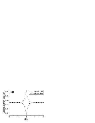
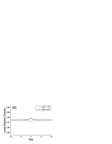
Figure 2: The local electron density along $x$-axis when an impurity is located at 0: (a) a type-(ii) impurity ($t$-variation), (b) a type-(iii) impurity ($J$-variation).

We thank C.-M. Ho for discussion.

References

- Kohsaka (07) Y. Kohsaka et al., Science 315 (2007) 1380.
- Anderson (00) P. W. Anderson, Science 228 (2000) 408.
- QH Wang (06) Q.-H. Wang et al., Phys. Rev. B 73 (2006) 092507.
- C Li (06) C. Li et al., Phys. Rev. B 73 (2006) 060501.
- Tsuchiura (00) H. Tsuchiura et al., Phys. Rev. Lett. 84 (2000) 3165.