Multicritical Behavior in a Random-Field Ising Model under a Continuous-Field Probability Distribution

Abstract

A random-field Ising model that is capable of exhibiting a rich variety of multicritical phenomena, as well as a smearing of such behavior, is investigated. The model consists of an infinite-range-interaction Ising ferromagnet in the presence of a triple-Gaussian random magnetic field, which is defined as a superposition of three Gaussian distributions with the same width $\sigma$, centered at $H=0$ and $H=\pm H_{0}$, with probabilities $p$ and $(1-p)/2$, respectively. Such a distribution is very general and recovers as limiting cases, the trimodal, bimodal, and Gaussian probability distributions. In particular, the special case of the random-field Ising model in the presence of a trimodal probability distribution (limit $\sigma\rightarrow 0$) is able to present a rather nontrivial multicritical behavior. It is argued that the triple-Gaussian probability distribution is appropriate for a physical description of some diluted antiferromagnets in the presence of a uniform external field, for which the corresponding physical realization consists of an Ising ferromagnet under random fields whose distribution appears to be well-represented in terms of a superposition of two parts, namely, a trimodal and a continuous contribution. The model is investigated by means of the replica method, and phase diagrams are obtained within the replica-symmetric solution, which is known to be stable for the present system. A rich variety of phase diagrams is presented, with a single or two distinct ferromagnetic phases, continuous and first-order transition lines, tricritical, fourth-order, critical end points, and many other interesting multicritical phenomena. Additionally, the present model carries the possibility of destructing such multicritical phenomena due to an increase in the randomness, i.e., increasing $\sigma$, which represents a very common feature in real systems.

Keywords: Random-Field Ising Model, Multicritical Phenomena, Replica Method.

I INTRODUCTION

The Random Field Ising Model (RFIM) became nowadays one of the most studied problems in the area of disordered magnetic systems youngbook ; dotsenkobook . From the theoretical point of view nattermannreview , its simple definition imryma , together with the richness of physical properties that emerge from its study, represent two main motivations for the investigation of this model. On the other hand, a considerable experimental interest belangerreview arised after the identification of the RFIM with diluted antiferromagnets in the presence of a uniform magnetic field fishmanaharony ; pozenwong ; cardy ; since then, two of the most investigated systems are the compounds ${\rm Fe_{x}Zn_{1-x}F_{2}}$ and ${\rm Fe_{x}Mg_{1-x}Cl_{2}}$ belangerreview ; birgeneau .

In what concerns the equilibrium phase diagrams of the RFIM, the effects of different probability-distribution functions (PDFs) for the random fields have attracted the attention of many authors, see, e.g., Refs. schneiderpytte ; aharony78 ; andelman ; galambirman ; mattis ; kaufman ; nuno08a ; aizenman ; huiberker ; gofman ; swift ; machta00 ; middleton ; machta03 ; wumachta05 ; wumachta06 ; fytas , among others. At the mean-field level, the Gaussian PDF yields a continuous ferromagnetic-paramagnetic boundary schneiderpytte , whereas discrete PDFs may lead to elaborate phase diagrams, characterized by a finite-temperature tricritical point followed by a first-order phase transition at low temperatures aharony78 ; andelman ; galambirman ; mattis ; kaufman , or even fourth-order and critical end points mattis ; kaufman . For the short-range-interaction RFIM, the existence of a low-temperature first-order phase transition remains a very controversial issue aizenman ; huiberker ; gofman ; swift ; machta00 ; middleton ; machta03 ; wumachta05 ; wumachta06 ; fytas .

From the experimental point of view, one is certainly concerned with physical realizations of the RFIM, for which the most commonly known are diluted antiferromagnets in the presence of a uniform magnetic field belangerreview . Hence, in the identification of RFIMs with such real systems fishmanaharony ; pozenwong ; cardy , certain classes of distributions for the random fields, in the corresponding RFIM, are more appropriate for a description of diluted antiferromagnets in the presence of a uniform magnetic field. In the later systems one has local variations in the sum of exchange couplings that connect a given site to other sites, leading to local variations of the two-sublattice site magnetizations, and as a consequence, one may have local magnetizations that vary in both sign and magnitude. In the identifications of the RFIM with diluted antiferromagnets fishmanaharony ; pozenwong ; cardy , the effective random field at a given site is expressed always in terms of quantities that vary in both sign and magnitude: (i) the local magnetization fishmanaharony ; (ii) two contributions, namely, a first one that assumes only three discrete values, related to the dilution of the system and the uniform external field, and a second one that is proportional to the local magnetization pozenwong ; (iii) the sum of the exchange couplings associated to this site cardy . Therefore, for a proper description of diluted antiferromagnets in the presence of a uniform field, the corresponding RFIMs should always be considered in terms of continuous PDFs for the fields.

The compound ${\rm Fe_{x}Mg_{1-x}Cl_{2}}$ presents an Ising spin-glass behavior for ${\rm x}<0.55$, and is considered as a typical RFIM for higher magnetic concentrations. In the RFIM regime, it shows some curious behavior and is considered as a candidate for exhibiting multicritical phenomena belangerreview ; pozenwong ; kaufman . As an example of this type of effect, one finds a first-order transition turning into a continuous one due to a change in the random fields belangerreview ; kushauerkleemann ; kushauer ; the concentration at which the first-order transition disappears is estimated to be $x=0.6$. The crossover from first-order to continuous phase transitions has been investigated through different theoretical approaches aizenman ; huiberker ; kushauer . One possible mechanism used to find such a crossover, or even to suppress the first-order transition completely, consists in introducing an additional kind of randomness in the system, e.g., bond randomness aizenman ; huiberker . By considering randomness in the field only, this crossover has been also analyzed through zero-temperature studies, either within mean-field theory sethna93 , or numerical simulations on a three-dimensional lattice kushauer ; sethna93 . Recently a RFIM has been proposed nuno08a for which the finite-temperature tricritical point, together with the first-order line, may disappear due to an increase in the field randomness, similarly to what happens with the first-order phase transition in the compound ${\rm Fe_{x}Mg_{1-x}Cl_{2}}$.

However, it is possible that the diluted antiferromagnet ${\rm Fe_{x}Mg_{1-x}Cl_{2}}$, or some other similar compound, may present an even more complicated critical behavior, not yet verified experimentally, to our knowledge. According to the analysis of Ref. pozenwong , one of its contributions for the random fields assumes only the values $0,\pm\sqrt{2}H$ ($H$ represents the external uniform magnetic field); motivated by this result, a RFIM was proposed mattis ; kaufman with the random fields described in terms of a trimodal distribution. Such a RFIM, studied within a mean-field approach through a model defined in the limit of infinite-range interactions, yielded a rich critical behavior with the occurence of first-order phase transitions, tricritical and high-order critical points griffiths at finite temperatures, and even the possibility of two distinct ferromagnetic phases at low temperatures mattis ; kaufman . These investigations suggest that ${\rm Fe_{x}Mg_{1-x}Cl_{2}}$ may exhibit a rich critical behavior that goes beyond the disappearance of a first-order phase transition observed around $x=0.6$. However, taking into account the above criteria for the identification of the RFIM with diluted antiferromagnets, one notices that the trimodal distribution does not represent an appropriate choice from the physical point of view. In fact, in the analysis of Ref. pozenwong , a second, continuous contribution for the random fields should be taken into account as well. Therefore, for an adequate theoretical description of ${\rm Fe_{x}Mg_{1-x}Cl_{2}}$, one should consider a RFIM defined in terms of a finite-width three-peaked distribution, which could exhibit multicritical behavior, and in addition to that, a crossover from such behavior to continuous phase transitions due to an increase in the field randomness.

For that purpose, herein we introduce a RFIM that consists of an infinite-range-interaction Ising ferromagnet in the presence of a triple-Gaussian random magnetic field. This distribution is defined as a superposition of three Gaussian distributions with the same width $\sigma$, centered at $H=0$ and $H=\pm H_{0}$, with probabilities $p$ and $(1-p)/2$, respectively. The particular case of the RFIM in the presence of a trimodal PDF, studied previously mattis ; kaufman , is recovered in the limit $\sigma\rightarrow 0$. We show that the present model is capable of exhibiting a rich multicritical behavior, with phase diagrams displaying one, or even two distinct ferromagnetic phases, continuous and first-order critical frontiers, tricritical points and high-order critical points, at both finite and zero temperatures. Such a variety of phase diagrams may be obtained from this model by varying the parameters of the corresponding PDF, e.g., $p$ and $\sigma$: (i) Variations in $p$ ($\sigma$ fixed) lead to qualitatively distinct multicritical phenomena; (ii) Increasing $\sigma$ ($p$ fixed) yields a smearing of an specific type of critical behavior, destroying a possible multicritical phenomena due to an increase in the randomness, representing a very common feature in real systems. In the next section we define the model, find its free energy and equation for the magnetization, by using the replica approach. In section III we present several phase diagrams, characterized by the critical behavior mentioned above. Finally, in section IV we present our conclusions.

II THE MODEL

The infinite-range-interaction Ising model in the presence of an external random magnetic field is defined in terms of the Hamiltonian

$$\mathcal{H}=-\frac{J}{N}\sum_{(i,j)}S_{i}S_{j}-\sum_{i}H_{i}S_{i}~{},$$ (1)

where the sum $\sum_{(i,j)}$ runs over all distinct pairs of spins $S_{i}=\pm 1$ ($i=1,2,...,N$). The random fields $\{H_{i}\}$ are quenched variables and obey the PDF,

$$P(H_{i}) = \frac{(1-p)}{2}\left(\frac{1}{2\pi\sigma^{2}}\right)^{1/2}\left\{\exp\left[-\frac{(H_{i}-H_{0})^{2}}{2\sigma^{2}}\right]+\exp\left[-\frac{(H_{i}+H_{0})^{2}}{2\sigma^{2}}\right]\right\}$$ (2)

$$+ p\left(\frac{1}{2\pi\sigma^{2}}\right)^{1/2}\exp\left[-\frac{H_{i}^{2}}{2\sigma^{2}}\right]~{},$$

which consists of a superposition of three independent Gaussian distributions with the same width $\sigma$, centered at $H_{i}=0$ and $H_{i}=\pm H_{0}$, with probabilities $p$ and $(1-p)/2$, respectively (to be called hereafter, a triple Gaussian PDF). This distribution is very general, depending on three parameters, namely, $p$, $\sigma$, and $H_{0}$, and contains as particular cases several well-known distributions of the literature, namely the trimodal and bimodal distributions, the double Gaussian, as well as simple Gaussian distributions. The model defined above is expected to be appropriate for a physical description of diluted antiferromagnets that in the presence of an external magnetic field may exhibit multicritical behavior; one candidate for this purpose is ${\rm Fe_{x}Mg_{1-x}Cl_{2}}$ pozenwong .

From the free energy $F(\{H_{i}\})$, associated with a given realization of site fields $\{H_{i}\}$, one may calculate the quenched average, $[F(\{H_{i}\})]_{H}$,

$$[F(\{H_{i}\})]_{H}=\int\prod_{i}[dH_{i}P(H_{i})]F(\{H_{i}\})~{}.$$ (3)

The standard procedure for carrying the average above is by making use of the replica method dotsenkobook ; nishimoribook , leading to the free energy per spin,

$$-\beta f=\lim_{N\to\infty}\frac{1}{N}[\ln Z(\{H_{i}\})]_{H}=\lim_{N\to\infty}\lim_{n\to 0}\frac{1}{Nn}([Z^{n}]_{H}-1)~{},$$ (4)

where $Z^{n}$ is the partition function of $n$ copies of the original system defined in Eq. (1) and $\beta=1/(kT)$. One gets that,

$$\beta f=\lim_{n\to 0}\frac{1}{n}\,{\rm min}\;g(m^{\alpha})~{},$$ (5)

with

$$g(m^{\alpha}) = \frac{\beta J}{2}\sum_{\alpha}(m^{\alpha})^{2}-\frac{(1-p)}{2}\ln{\rm Tr}_{\alpha}\exp(\mathcal{H}_{{\rm eff}}^{+})-\frac{(1-p)}{2}\ln{\rm Tr}_{\alpha}\exp(\mathcal{H}_{{\rm eff}}^{-})$$ (6)

$$- p\ln{\rm Tr}_{\alpha}\exp(\mathcal{H}_{{\rm eff}}^{(0)})~{},$$

$$\mathcal{H}_{{\rm eff}}^{\pm} = \beta J\sum_{\alpha}m^{\alpha}S^{\alpha}+\beta\sigma\left(\sum_{\alpha}S^{\alpha}\right)^{2}\pm\beta H_{0}\sum_{\alpha}S^{\alpha}~{},$$ (7)

$$\mathcal{H}_{{\rm eff}}^{(0)} = \beta J\sum_{\alpha}m^{\alpha}S^{\alpha}+\beta\sigma\left(\sum_{\alpha}S^{\alpha}\right)^{2}~{}.$$ (8)

In the equations above, $\alpha$ represents a replica label ($\alpha=1,2,...,n$) and ${\rm Tr}_{\alpha}$ stands for a trace over the spin variables of each replica. The extrema of the functional $g(m^{\alpha})$ leads to the equation for the magnetization of replica $\alpha$,

$$m^{\alpha}=\frac{(1-p)}{2}<S^{\alpha}>_{+}\ +\ \frac{(1-p)}{2}<S^{\alpha}>_{-}\ +\ p<S^{\alpha}>_{0}~{},$$ (9)

where $<\,>_{\pm}$ and $<\,>_{0}$ denote thermal averages with respect to the “effective Hamiltonians” $\mathcal{H}_{{\rm eff}}^{\pm}$ and $\mathcal{H}_{{\rm eff}}^{(0)}$, in Eqs. (7) and (8), respectively.

If one assumes the replica-symmetry ansatz dotsenkobook ; nishimoribook , i.e., $m^{\alpha}=m$ ($\forall~{}\alpha$), the free energy per spin of Eqs. (5)–(8) and the equilibrium condition, Eq. (9), become

$$f = \frac{J}{2}m^{2}-\frac{(1-p)}{2\beta}\int Dz\ln(2\cosh\Phi^{+})-\frac{(1-p)}{2\beta}\int Dz\ln(2\cosh\Phi^{-})$$ (10)

$$- \frac{p}{2}\int Dz\ln(2\cosh\Phi^{(0)})~{},$$

$$m = \frac{(1-p)}{2}\int Dz\tanh\Phi^{+}+\frac{(1-p)}{2}\int Dz\tanh\Phi^{-}+p\int Dz\tanh\Phi^{(0)}~{},$$ (11)

where

$$\Phi^{\pm}=\beta(Jm+\sigma z\pm H_{0})~{};\quad\Phi^{(0)}=\beta(Jm+\sigma z)~{};\quad\int Dz\;(..)=\frac{1}{\sqrt{2\pi}}\int_{-\infty}^{+\infty}dz\;e^{-z^{2}/2}\;(..)~{}.$$ (12)

It should be mentioned that the instability associated with the replica-symmetric solution at at low temperatures is usually related to parameters characterized by two replica indices, like in the spin-glass problem dotsenkobook ; nishimoribook . In the present system the order parameter $m^{\alpha}$ depends on a single replica index, and so such an instability does not occur.

In the next section we will make use of Eqs. (10) and (11) in order to get several phase diagrams for the present model. Although most critical frontiers will be achieved numerically, some analytical results may be obtained at zero temperature. At $T=0$, the free energy and magnetization become, respectively,

$$f = -\frac{J}{2}m^{2}-\frac{H_{0}}{2}(1-p)\left[{\rm erf}\left(\frac{Jm+H_{0}}{\sigma\sqrt{2}}\right)-{\rm erf}\left(\frac{Jm-H_{0}}{\sigma\sqrt{2}}\right)\right]$$ (13)

$$- \frac{\sigma}{\sqrt{2\pi}}(1-p)\left\{\exp\left[-\frac{(Jm+H_{0})^{2}}{2\sigma^{2}}\right]+\exp\left[-\frac{(Jm-H_{0})^{2}}{2\sigma^{2}}\right]\right\}$$

$$- \frac{2\sigma}{\sqrt{2\pi}}\;p\exp\left[-\frac{(Jm)^{2}}{2\sigma^{2}}\right]~{},$$

$$m=\frac{(1-p)}{2}~{}{\rm erf}\left(\frac{Jm+H_{0}}{\sigma\sqrt{2}}\right)+\frac{(1-p)}{2}~{}{\rm erf}\left(\frac{Jm-H_{0}}{\sigma\sqrt{2}}\right)+p\;{\rm erf}\left(\frac{Jm}{\sigma\sqrt{2}}\right)~{}.$$ (14)

III PHASE DIAGRAMS

Usually, in the RFIM one has two phases, namely, the Ferromagnetic (F) and Paramagnetic (P) ones. However, for the PDF of Eq. (2), there is a possibility of three distinct phases: apart from the Paramagnetic ($m=0$), one has two Ferromagnetic phases, F$\!{}_{1}$ and F$\!{}_{2}$ , characterized by different magnetizations (herein we will consider always F$\!{}_{1}$ as the ordered phase with higher magnetization, i.e., $m_{1}>m_{2}>0$). Close to a continuous transition between an ordered and the disordered phases, $m$ is small, so that one can expand Eq. (11) in powers of $m$,

$$m=A_{1}m+A_{3}m^{3}+A_{5}m^{5}+A_{7}m^{7}+0(m^{9})~{},$$ (15)

where the coefficients are given by

$$A_{1} = \beta J\{1-(1-p)\lambda_{1}-p\lambda_{1}^{(0)}\}~{},$$ (16)

$$A_{3} = -\frac{(\beta J)^{3}}{3}\{1-4[(1-p)\lambda_{1}+p\lambda_{1}^{(0)}]+3[(1-p)\lambda_{2}+p\lambda_{2}^{(0)}]\}~{},$$ (17)

$$A_{5} = \frac{(\beta J)^{5}}{15}\{2-17[(1-p)\lambda_{1}+p\lambda_{1}^{(0)}]+30[(1-p)\lambda_{2}+p\lambda_{2}^{(0)}]-15[(1-p)\lambda_{3}$$ (18)

$$+ p\lambda_{3}^{(0)}]\}~{}$$

$$A_{7} = \frac{(\beta J)^{7}}{315}\{17-248[(1-p)\lambda_{1}+p\lambda_{1}^{(0)}]+756[(1-p)\lambda_{2}+p\lambda_{2}^{(0)}]-840[(1-p)\lambda_{3}$$ (19)

$$+ p\lambda_{3}^{(0)}]+315[(1-p)\lambda_{4}+p\lambda_{4}^{(0)}]\}~{},$$

with

$$\lambda_{k} = \frac{1}{\sqrt{2\pi}}\int_{-\infty}^{+\infty}dz\;e^{-z^{2}/2}\tanh^{2k}\beta(H_{0}+\sigma z)~{},$$

$$\lambda_{k}^{(0)} = \frac{1}{\sqrt{2\pi}}\int_{-\infty}^{+\infty}dz\;e^{-z^{2}/2}\tanh^{2k}(\beta\sigma z)~{}.$$ (20)

In order to find the continuous critical frontier one sets $A_{1}=1$, provided that $A_{3}<0$. If a first-order critical frontier also occurs, the continuous line ends when $A_{3}=0$; in such cases, the continuous and first-order critical frontiers meet at a tricritical point, whose coordinates may be obtained by solving the equations $A_{1}=1$ and $A_{3}=0$ numerically, provided that $A_{5}<0$. In the present problem there is also a possibility of a fourth-order critical point, which is obtained from the conditions $A_{1}=1$, $A_{3}=A_{5}=0$ and $A_{7}<0$. In addition, when the two distinct ferromagnetic phases are present, two other critical points may also appear (herein we follow the classification due to Griffithis griffiths ): (i) the ordered critical point, which corresponds to an isolated critical point inside the ordered region, terminating a first-order line that separates phases F$\!{}_{1}$ and F$\!{}_{2}$ ; (ii) the critical end point, where all three phases coexist, corresponding to the intersection of a continuous line that separates the paramagnetic from one of the ferromagnetic phases with a first-order line separating the paramagnetic and the other ferromagnetic phase. The location of the critical points defined in (i) and (ii), as well as the first-order critical frontiers, were determined by a numerical analysis of the free-energy minima, e.g., two equal minima for the free energy, characterized by two different values of magnetization, $m_{1}>m_{2}>0$, yields a point of the first-order critical frontier separating phases F$\!{}_{1}$ and F$\!{}_{2}$ .

Next, we show several phase diagrams of this model for both finite and zero temperatures. Besides the notation defined above for labeling the phases, in these phase diagrams we shall use distinct symbols and representations for the critical points and frontiers, as described below.

• Continuous critical frontier: continuous line;

• First-order critical frontier: dotted line;

• Tricritical point: located by a black circle;

• Fourth-order point: located by an empty square;

• Ordered critical point: located by a black asterisk;

• Critical end point: located by a black triangle.

III.1 Finite-Temperature Critical Frontiers

We now present finite-temperature phase diagrams; these phase diagrams will be exhibited in the plane of dimensionless variables, $(kT)/J$ versus $H_{0}/J$, for typical values of $p$ and $\sigma/J$. For completeness, in each figure we also show the forms of the corresponding PDF of Eq. (2), with the parameters used in the phase diagrams.

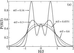
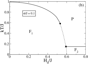
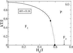
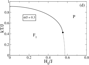
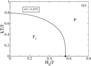
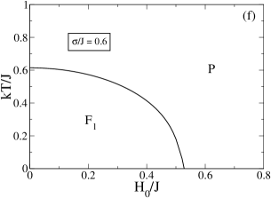
Figure 1: (a) The probability distribution of Eq. (2), for $p=0.2$ and $(H_{0}/J)=0.56$ is represented for several values of its width. (b)–(f) Phase diagrams showing the critical frontiers separating the paramagnetic (P) and ferromagnetic (F$\!{}_{1}$ and F$\!{}_{2}$) phases of the infinite-range-interaction ferromagnet in the presence of a triple Gaussian random field, for typical values of $\sigma/J$ and $p=0.2$. Critical frontiers and critical points are as described in the text. All quantities are scaled in units of $J$.

In Fig. 1 we present some qualitatively distintic phase diagrams of the model, for the fixed value $p=0.2$ and typical values of $\sigma/J$. In Fig. 1(a) we represent the PDF of Eq. (2) for $p=0.2$, $(H_{0}/J)=0.56$, and the widths $\sigma/J$ used to obtain the phase diagrams of Figs. 1(c)–(f). The particular case $(\sigma/J)=0.1$, used in Fig. 1(b), yields a three-narrow-peaked distribution and is not represented in Fig. 1(a) for a better visualization of the remaining cases; in addition to that, the choice $(H_{0}/J)=0.56$ corresponds to a region in the phase diagrams where essential changes occur in the criticality of the system at low temperatures. One notices that the critical frontier separating the paramagnetic (P) and ferromagnetic (F$\!{}_{1}$ and F$\!{}_{2}$) phases exhibits significant changes with increasing values of $\sigma/J$. For $(\sigma/J)=0.1$ [cf. Fig. 1(b)], one has a phase diagram that is qualitatively similar to the one obtained in the case of the trimodal distribution kaufman , with a tricritical point (black circle) and a critical end point (black triangle) at a lower, but finite temperature, where the critical frontier separating phases P and F$\!{}_{2}$ meets the first-order line. However, for increasing values of $\sigma/J$ these critical points move towards low temperatures, in such a way that for $(\sigma/J)=0.16$ one observes the collapse of the critical end point with the zero-temperature axis, i.e., the ferromagnetic phase F$\!{}_{2}$ occurs only for $T=0$, as shown in Fig. 1(c). Therefore, for $p=0.2$ the value $(\sigma/J)=0.16$ represents a threshold for the existence of phase F$\!{}_{2}$. One should notice from Fig. 1(a), that for $p=0.2$, the existence of the phase F$\!{}_{2}$ is associated with a PDF for the fields characterized by a three-peaked shape. For $(\sigma/J)=0.3$ [cf. Fig. 1(d)], the phase diagram is qualitatively similar to the one obtained for the bimodal aharony78 or continuous two-peaked distributions nuno08a , where one finds a tricritical point at finite temperatures and a first-order transition at lower temperatures. We have found analitically through a zero-temperature analysis that will be discussed later, the value $(\sigma/J)\cong 0.4551$ for which the tricritical point reaches the zero-temperature axis, signaling a complete destruction of the first-order phase transition in the case $p=0.2$, as exhibited in Fig. 1(e). In this case, the associated PDF presents a single flat maximum in agreement with Refs. aharony78 ; andelman ; galambirman . For even higher values of $\sigma/J$, as shown in Fig. 1(f) for the case $(\sigma/J)=0.6$, the PDF presents a single peak, and the frontier ferromagnetic-paramagnetic is completely continuous, qualitatively similar to the case of a single Gaussian PDF schneiderpytte .

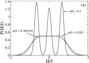
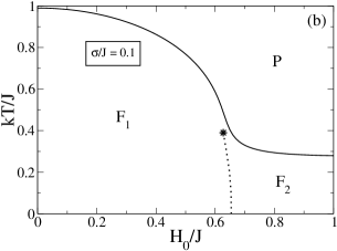
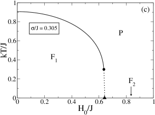
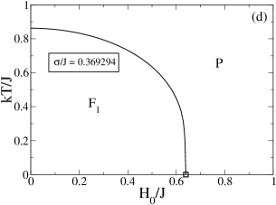
Figure 2: (a) The probability distribution of Eq. (2), for $p=0.308561$ and $(H_{0}/J)=0.65$, is represented for several values of its width. (b)–(d) Phase diagrams showing the critical frontiers separating the paramagnetic (P) and ferromagnetic (F$\!{}_{1}$ and F$\!{}_{2}$) phases of the infinite-range-interaction ferromagnet in the presence of a triple Gaussian random field, for typical values of $\sigma/J$ and $p=0.308561$. Critical frontiers and critical points are as described in the text. All quantities are scaled in units of $J$.

There is an special value of $p$, to be denoted herein $p^{*}$, which represents an upper limit for the existence of tricritical points along the paramagnetic border, characterized by a fourth-order point at zero temperature. The value $p^{*}\cong 0.308561$, as well as its associated width, $(\sigma^{*}/J)\cong 0.369294$, will be determined later, within a zero-temperature analysis. In Fig. 2 we show phase diagrams for $p=0.308561$ and three different values of $\sigma/J$. In Fig. 2(a) we represent the PDF of Eq. (2) for $p=0.308561$, $(H_{0}/J)=0.65$, and the widths $\sigma/J$ used to obtain the phase diagrams of Figs. 2(b)–(d); the choice $(H_{0}/J)=0.65$ has to do with a region in the phase diagrams where interesting critical phenomena occur at low temperatures. In Fig. 2(b) we present the phase diagram for $(\sigma/J)=0.1$, where one sees that the border of the paramagnetic phase is completely continuous; for lower (higher) fields this critical frontier separates phases P and F$\!{}_{1}$ (F$\!{}_{2}$). However, there is a curious first-order line separating phases F$\!{}_{1}$ and F$\!{}_{2}$ that terminates in an ordered critical point (black asterisk), above which one can pass smoothly from one of these phases to the other. By slightly increasing the values of $\sigma/J$ one observes that the ordered critical point disappears, leading to the emergence of both tricritical and critical end points at finite temperatures, yielding a phase diagram that is qualitatively similar to the one shown in Fig. 1(b); this type of phase diagram occurs typically in the range $0.1<(\sigma/J)<0.3$. However, as shown in Fig. 2(c) for $(\sigma/J)=0.305$, one has the collapse of the critical end point with the zero-temperature axis, with the phase F$\!{}_{2}$ occurring at zero temperature only, analogous to the one that appears in Fig. 1(c), but now for a higher value of $H_{0}/J$. Comparing Figs. 1(c) and 2(c), one sees that in some cases, essentially similar phase diagrams may be obtained by increasing both $p$ and $\sigma/J$; however, in the case of higher values for these parameters, the extension of the first-order transition line gets reduced. It should be mentioned that, in both figures, the existence of the phase F$\!{}_{2}$ is associated with a PDF for the fields characterized by a three-peaked shape. In Fig. 2(d) we display the phase diagram for $(\sigma/J)=0.369294$, for which the first-order line is totally destroyed. It should be emphasized that this effect appears also for other values of $p$ through a tricritical point at $T=0$ [cf. Fig. 1(e)]; however, the phase diagram of Fig. 2(d) is very special, in the sense that the collapse of the first-order frontier with the zero-temperature axis occurs by means of a fourth-order point. For higher values of $\sigma/J$, the critical frontier separating phases P and F$\!{}_{1}$ is completely continuous, and one has essentially the same phase diagram shown in Fig. 1(f).

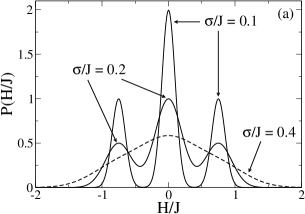
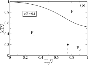
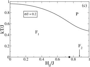
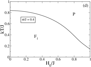
Figure 3: (a) The probability distribution of Eq. (2), for $p=0.5$ and $(H_{0}/J)=0.74$, is represented for several values of its width. (b)–(d) Phase diagrams showing the critical frontiers separating the paramagnetic (P) and ferromagnetic (F$\!{}_{1}$ and F$\!{}_{2}$) phases of the infinite-range-interaction ferromagnet in the presence of a triple Gaussian random field, for typical values of $\sigma/J$ and $p=0.5$. Critical frontiers and critical points are as described in the text. All quantities are scaled in units of $J$.

Additional phase diagrams are shown in Fig. 3, for the case $p=0.5$. In Fig. 3(a) we represent the PDF of Eq. (2) for such a value of $p$, $(H_{0}/J)=0.74$, and the widths $\sigma/J$ used to obtain the phase diagrams of Figs. 3(b)–(d); the choice $(H_{0}/J)=0.74$ corresponds to a region of the phase diagram where an ordered critical point appears at low temperatures. In Fig. 3(b) we present the phase diagram for the same $\sigma/J$ value of Figs. 1(b) and 2(b), i.e., $(\sigma/J)=0.1$; these figures suggest that the existence of phase F$\!{}_{2}$ is associated with three-peaked distributions. However, for sufficiently small $p$, this phase appears together with a critical end point, as shown in Fig. 1(b), whereas for larger $p$, the border of the paramagnetic phase is completely continuous, and phases F$\!{}_{1}$ and F$\!{}_{2}$ are separated by a first-order critical frontier that terminates in an ordered critical point. In Fig. 3(b) one can go smoothly from one of these two ferromagnetic phases to the other, through a thermodynamic path connecting these phases above the ordered critical point. In Fig. 3(c) one has the collapse of the ordered critical point with the zero-temperature axis, which was estimated numerically to occur for $(\sigma/J)=0.20$, with the phase F$\!{}_{2}$ appearing at zero temperature. It is important to mention that the phase diagram exhibited in Fig. 3(c) is qualitatively distinct from those of Figs. 1(c) and 2(c), in the sense that the first one is characterized by a border of the paramagnetic phase that is completely continuous and at zero temperature, phases F$\!{}_{1}$ and F$\!{}_{2}$ are separated by an ordered critical point. For the value $(\sigma/J)=0.4$ shown in Fig. 3(d), one gets a continuous critical frontier separating phases P and F$\!{}_{1}$. However, there is a basic difference between the phase diagrams displayed in Figs. 1(f) and 3(d): as it will be shown in the following zero-temperature analysis, in the later case there is no zero-temperature point separating these two phases, i.e., the phase F$\!{}_{1}$ exists for all values of $H_{0}/J$. In fact, for any $(\sigma/J)\leq 0.4$ the border of the paramagnetic phase never touches the zero-temperature axis, as suggested in Figs. 3(b)–(d); for higher values of $\sigma/J$, this critical line meets the $H_{0}/J$ axis, and one has a phase diagram qualitatively similar to the one of Fig. 1(f).

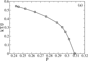
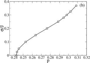
Figure 4: Projections of the fourth-order-point line on two different planes: (a) The plane $(kT)/J$ versus $p$, showing the critical temperatures associated with fourth-order points that exist in the interval $8/33\leq p\leq p^{*}$; (b) The plane $\sigma/J$ versus $p$. The empty squares are computed fourth-order points, whereas the lines (guides to the eye) represent lines of fourth-order points.

There are some important threshold values associated with the existence of the above-mentioned critical points, as described next.

(i) We found numerically that for $p\gtrsim p^{*}$, critical end points do not occur, either in finite or zero temperatures.

(ii) We verified, also numerically, that for $p\gtrsim 0.93$, ordered critical points cease to exist; as a consequence, this represents a threshold for the existence of phase F$\!{}_{2}$, which does not appear above this value (even at zero temperature).

(iii) In the zero-temperature analysis (to be carried below), we find analytically that for $p^{*}\cong 0.308561$ one gets a fourth-order point at zero temperature; this value depicts an upper bound for the existence of tricritical points.

(iv) Fourth-order points usually delimitate the existence of tricritical points and are sometimes considered in the literature as “vestigial” tricritical points kaufman . In the case of the power expansion in Eq. (15), they exist for finite temperatures as well, and are determined by the conditions $A_{1}=1$, $A_{3}=A_{5}=0$ and $A_{7}<0$, which define a line in the four-dimensional space $[(kT)/J,p,H_{0}/J,\sigma/J]$. In Fig. 4 we present projections of the fourth-order-point line with the planes $(kT)/J$ versus $p$ [Fig. 4(a)] and $\sigma/J$ versus $p$ [Fig. 4(b)]. These projections interpolate between the fourth-order points occurring for $p=8/33$ ($\sigma=0$, i.e., trimodal distribution kaufman ) and the zero-temperature threshold value for the triple Gaussian PDF, $p^{*}\cong 0.308561$, to be determined below.

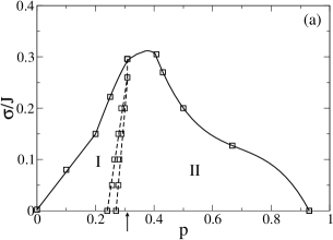
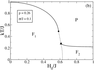
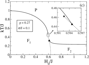
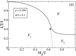
Figure 5: (a) Regions, in the plane $\sigma/J$ versus $p$, associated with qualitatively distinct phase diagrams for the present model; the empty squares represent computed points, whereas the lines are just guides to the eye; the arrow indicates the threshold value $p=p^{*}$. In regions I and II one has phase diagrams like those shown in (b) and (d), respectively. The two dashed lines that appear in (a) define a narrow intermediate region, exhibiting a phase diagram characterized by two critical end points and one ordered critical point along the paramagnetic border, like shown in (c). The type of phase diagram in the intermediate region appears when one varies the parameters of the distribution of Eq. (2) in such a way to go from region I to region II [as shown typically in the sequence (b), (c) and (d), for $(\sigma/J)=0.1$], and vice versa.

From the analysis above one concludes that it is possible to obtain qualitatively similar phase diagrams for different pairs of parameters $(p,\sigma/J)$. Essentially, these phase diagrams are defined by the presence of the different types of critical points that may appear in this model. The existence of tricritical points was already discussed in items (iii) and (iv) above, whereas the regions in the plane $\sigma/J$ versus $p$ associated with ordered and critical end points are exhibited in Fig. 5(a). Along the axis $(\sigma/J)=0$ our limits for the existence of critical end points ($0<p\lesssim 0.24$) and ordered critical points ($0.27\lesssim p\lesssim 0.93$) are in agreement with those estimated in Ref. kaufman ; in between these two regimes, a small region occurs, which is very subtle, from the numerical point of view, where two critical end points and one ordered critical point show up. This intermediate region gets reduced for increasing values of $\sigma/J$ and is delimited by the two dashed lines shown in Fig. 5(a). A typical phase diagram inside this region is shown in Fig. 5(c), which is characterized by a critical frontier separating phases P and F$\!{}_{1}$ that presents a continuous piece, followed by a first-order line at lower temperatures, with no tricritical point. It is important to stress that the type of phase diagram of Fig. 5(c) occurs in the particular case $(\sigma/J)=0$ for a range of values of $p$ right above $p=8/33\approx 0.24$, which represents the probability at which a fourth-order point occurs at finite temperatures kaufman . We have verified that a similar effect occurs for finite values of $\sigma/J$, in the sense that the narrow intermediate region of Fig. 5(a) corresponds to a region of points to the right of the projection of the fourth-order line in the plane $\sigma/J$ versus $p$ of Fig. 4(b). This intermediate region occurs whenever the fourth order point appears for finite temperatures and it becomes essentially undiscernible, from the computational point of view, as one approaches the threshold $p=p^{*}$, corresponding to the fourth-order point at zero temmperature; we verified numerically that this region disappears completely at the threshold $p=p^{*}$ [this aspect is reinforced in Fig. 5(d) where we present a phase diagram for $p$ slightly larger than $p=p^{*}$]. The fact that the intermediate region gets reduced for increasing values of $\sigma$ is expected, since one of the effects introduced by the parameter $\sigma$ is to destroy several types of multicritical behavior. In Fig. 5(a), region I is associated with phase diagrams that present a single critical end point, like the one of Fig. 5(b), whereas region II is associated with phase diagrams presenting a single ordered critical point, as shown in Fig. 5(d); one may go from region I to region II through the sequence of phase diagrams presented in Figs. 5(b)–(d). The ranges of $p$ values associated with these two regions diminish for increasing values of $\sigma/J$, as shown in Fig. 5(a); the computed points along the full lines (empty squares) represent upper limits (in $\sigma/J$) for regions I and II, in which cases the corresponding critical points appear at zero temperature. As typical examples, one has the ranges for the appearence of these points, $\sigma/J\leq 0.08\ (p=0.1)$ and $\sigma/J\leq 0.16\ (p=0.2)$, in region I, whereas $\sigma/J\leq 0.2\ (p=0.5)$ and $\sigma/J\leq 0.127\ (p\approx 0.6667)$, in region II. Therefore, for a given pair of parameters $(p,\sigma/J)$ one may predict the qualitative form of its corresponding phase diagram by using Fig. 5(a). Let us first consider one value of $p$ within the range $0<p\lesssim 0.24$, where one may have both a critical end point and a tricritical point, e.g., the case $p=0.2$, discussed previously. Then, for sufficiently low values of $\sigma/J$ one has a phase diagram like the one shown in Fig. 1(b), characterized by a tricritical point, a first-order line at low temperatures and a critical end point, associated with a phase F$\!{}_{2}$; by increasing $\sigma/J$, one reaches the upper limit of region I [represented by the continuous line in Fig. 5(a)] that corresponds to a collapse of the critical end point with the zero-temperature axis, like shown in Fig. 1(c). Increasing $\sigma/J$ further, in such a way that the probability distribution for the fields still presents a minimum at $H=0$, one has a tricritical point at finite temperatures [with a typical phase diagram exhibited in Fig. 1(d)], and after that, one gets phase diagrams like those shown in Figs. 1(e) and (f). This sequence of phase diagrams occurs for all values of $p$ within this range. Now, if one considers $0.27\lesssim p<p^{*}$ in Fig. 5(a), by increasing $\sigma$ gradually one gets first a typical phase diagram characterized by an ordered critical point, like the one shown in Fig. 2(b), and then, one may go through the intermediate region between the two dashed lines, with a phase diagram as presented in Fig. 5(c), and afterwards, one follows a similar sequence of phase diagrams like those shown in Figs. 1(b)–(f). The last two steps of the previous sequence of phase diagrams apply if one increases $\sigma/J$ in the range $0.24<p<0.27$. By varying $\sigma/J$ for $p$ within the range $p^{*}<p\lesssim 0.93$ one gets phase diagrams that follow the sequence shown in Figs. 3. Finally, for $0.93\lesssim p\leq 1.0$ one has a phase diagram typical of the Gaussian RFIM, i.e., a continuous phase transition separating the paramagnetic and ferromagnetic phases.

III.2 Zero-Temperature Critical Frontiers

Some analytical results may be obtained from the investigation of the free energy and magnetization at zero temperature, given by Eqs. (13) and (14), respectively. Herein, we shall restrict ourselves to $\sigma>0$ in Eq. (2); the case $\sigma=0$, i.e., a trimodal PDF requires a separate analysis and the results are already known mattis ; kaufman .

For that purpose, one applies the same procedure described above for finite temperatures, starting with the expansion of Eq. (14) in powers of $m$,

$$m=a_{1}m+a_{3}m^{3}+a_{5}m^{5}+a_{7}m^{7}+O(m^{9})~{},$$ (21)

where

$$a_{1} = \sqrt{\frac{2}{\pi}}\left(\frac{J}{\sigma}\right)\left\{p+(1-p)\exp\left(-\frac{H_{0}^{2}}{2\sigma^{2}}\right)\right\}~{},$$ (22)

$$a_{3} = \frac{1}{6}\sqrt{\frac{2}{\pi}}\left(\frac{J}{\sigma}\right)^{3}\left\{(1-p)\left[\left(\frac{H_{0}}{\sigma}\right)^{2}-1\right]\exp\left(-\frac{H_{0}^{2}}{2\sigma^{2}}\right)-p\right\}~{},$$ (23)

$$a_{5} = \frac{1}{120}\sqrt{\frac{2}{\pi}}\left(\frac{J}{\sigma}\right)^{5}\left\{(1-p)\left[\left(\frac{H_{0}}{\sigma}\right)^{4}-6\left(\frac{H_{0}}{\sigma}\right)^{2}+3\right]\exp\left(-\frac{H_{0}^{2}}{2\sigma^{2}}\right)+3p\right\}$$ (24)

$$a_{7} = \frac{1}{5040}\sqrt{\frac{2}{\pi}}\left(\frac{J}{\sigma}\right)^{7}\Bigg{\{}(1-p)\left[\left(\frac{H_{0}}{\sigma}\right)^{6}-15\left(\frac{H_{0}}{\sigma}\right)^{4}+45\left(\frac{H_{0}}{\sigma}\right)^{2}-15\right]$$ (25)

$$\times\exp\left(-\frac{H_{0}^{2}}{2\sigma^{2}}\right)-15p\Bigg{\}}~{}.$$

A continuous critical frontier occurs at zero temperature according to the conditions, $a_{1}=1$ and $a_{3}<0$, leading to a relation involving $H_{0}/J$, $\sigma/J$ and $p$,

$$\frac{\sigma}{J}=\sqrt{\frac{2}{\pi}}\left\{p+(1-p)\exp\left[-\frac{1}{2}\left(\frac{H_{0}}{J}\right)^{2}\left(\frac{J}{\sigma}\right)^{2}\right]\right\}~{}.$$ (26)

One notices that, for $(H_{0}/J)=0$ one has $(\sigma/J)=\sqrt{2/\pi}\cong 0.7979\ (\forall p)$, yielding a continuous critical frontier for small values of $H_{0}/J$. For $a_{3}>0$, one gets a first-order critical frontier at zero-temperature, which is usually associated with higher-order critical points at finite temperatures. A tricritical point appears at zero-temperature, provided that $a_{1}=1$, $a_{3}=0$, and $a_{5}<0$, in such a way that,

$$\frac{H_{0}}{\sigma}=\left[1-\sqrt{\frac{2}{\pi}}\left(\frac{J}{\sigma}\right)p\right]^{-1/2}~{}.$$ (27)

Let us now analyze the coefficient $a_{5}$ under the conditions $a_{1}=1$, $a_{3}=0$. Substituting Eqs (26) and (27) in Eq. (24), one gets

$$a_{5}=\frac{1}{120}\left(\frac{J}{\sigma}\right)^{4}\left\{\left[1-\sqrt{\frac{2}{\pi}}\left(\frac{J}{\sigma}\right)p\right]^{-1}-3\right\}~{},$$ (28)

leading to $a_{5}<0$ for $\left[1-\frac{2}{\pi}\left(\frac{J}{\sigma}\right)p\right]^{-1}$ $<$ $3$. One should notice that for $p=0$, i.e., for a double-Gaussian PDF nuno08a , the coefficient $a_{5}$ is always negative; however, in the present case one may have $a_{5}=0$, in such a way that one has the possibility of a fourth-order critical point. This zero-temperature point is unique for the distribution of Eq. (2) and it occurs for a set of parameters $(p^{*},H_{0}^{*}/J,\sigma^{*}/J)$, to be determined below. Considering $a_{5}=0$,

$$\frac{\sigma}{J}=\frac{3}{2}\sqrt{\frac{2}{\pi}}\ p~{},$$ (29)

and using this result in Eq. (27), one gets

$$\frac{H_{0}}{\sigma}=\sqrt{3}~{}.$$ (30)

Taking $a_{3}=0$ and using Eqs. (29) and (30) leads to

$$p^{*}=2~{}(2+e^{3/2})^{-1}\cong 0.308561~{},$$ (31)

which may be substituted in Eqs. (29), (30) to yield, respectively,

$$\frac{\sigma^{*}}{J}=\frac{6}{\sqrt{2\pi}}~{}(2+e^{3/2})^{-1}\cong 0.369294~{};\quad\frac{H^{*}_{0}}{J}=3\sqrt{\frac{6}{\pi}}~{}(2+e^{3/2})^{-1}\cong 0.639637~{}.$$ (32)

Therefore, for the set of parameters of Eqs. (31) and (32) one has a fourth-order critical point at zero temperature, as shown previously in Fig. 2(d), and also exhibited in the zero-temperature phase diagram of Fig. 6. In the present problem, the zero-temperature fourth-order critical point may be interpreted as the threshold for the existence of tricritical points in both finite and zero temperatures. For $p>p^{*}$, there is no tricritical point for arbitrary values of $\sigma/J$ and $H_{0}/J$, although an ordered critical point may still occur for finite temperatures [cf. Fig. 3(b)], as well as at zero temperature [see Fig. 6]. This threshold is associated with a very flat PDF, as shown in Fig. 2(a), which is in agreement with the conditions for the existence of tricritical points aharony78 ; andelman ; galambirman .

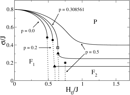
Figure 6: Zero-temperature phase diagrams of the infinite-range-interaction ferromagnet in the presence of a triple Gaussian random field, for typical values of $p$. The critical frontiers separate the paramagnetic (P) and ferromagnetic (F$\!{}_{1}$ and F$\!{}_{2}$) phases. Critical frontiers and critical points are as described in the text.

Zero-temperature phase diagrams of the model are presented in Fig. 6 for several values of $p$. One notices that besides tricritical, and the above-mentioned fourth-order point, critical end points and ordered critical points also appear at $T=0$. These two later points were determined by an analysis of the zero-temperature free energy of Eq. (13), similarly to what was done for finite temperatures. Comparing the phase diagrams of Fig. 6 with those for finite temperatures, one notices that the width $\sigma$ produces disorder, playing a role at $T=0$ that is similar to the temperature; as examples, one sees that the phase diagrams for $p=0$, $p=0.2$, and $p=0.5$, in Fig. 6, resemble those shown in Figs. 1(d), 1(b), and 3(b), respectively, if one considers the correspondence $\sigma\leftrightarrow T$.

IV CONCLUSIONS

We have investigated a random-field Ising model that consists of an infinite-range-interaction Ising ferromagnet in the presence of a random magnetic field following a triple-Gaussian probability distribution. Such a distribution, which is defined as a superposition of three Gaussian distributions with the same width $\sigma$, centered at $H=0$ and $H=\pm H_{0}$, with probabilities $p$ and $(1-p)/2$, respectively, is very general and recovers as limiting cases, the trimodal, bimodal, and Gaussian probability distributions. We have shown that this model is capable of exhibiting a rich variety of multicritical phenomena, essentially all types of critical phenomena found in previous RFIM investigations (as far as we know). We have obtained several phase diagrams, for finite temperatures, by varying the parameters of the corresponding probability distribution, e.g., $p$ and $\sigma$, with variations in $p$ ($\sigma$ fixed) leading to qualitatively distinct multicritical phenomena, whereas increasing $\sigma$ ($p$ fixed) yields a smearing of an specific type of critical behavior.

The random-field Ising model defined in terms of a trimodal probability distribution mattis ; kaufman represents, to our knowledge, the previously investigated model that exhibits a variety of multicritical phenomena comparable to the one discussed above. Since the former represents a particular case ($\sigma=0$) of the present model, the parameter $\sigma$ may be considered as an additional parameter used herein, when compared with the model of Refs. mattis ; kaufman . It is important to stress the relevance of this additional parameter for the richness of the phase diagrams, as well as for possible physical applications. As one illustration of the phase diagrams, one may mention those obtained through the zero-temperature analysis of the present model, where one gets a large variety of critical frontiers, exhibiting all types of critical points that occur at finite temperatures; this should be contrasted with the much simpler zero-temperature phase diagram of the trimodal random-field Ising model (where only an ordered critical point is possible). In particular, some of the zero-temperature phase diagrams presented herein resemble those for finite temperatures, if one considers the correspondence $\sigma\leftrightarrow T$. Therefore, $\sigma$ may be identified as a parameter directly related to the disorder in a real system, in such a way that an increase in $\sigma$ in the present model should play a similar role to an increase in the dilution for a diluted antiferromagnet nuno08a . It is important to remind that in the identifications of the RFIM with diluted antiferromagnets fishmanaharony ; pozenwong ; cardy , the effective random field at a given site is expressed always in terms of quantities that vary in both sign and magnitude, and so the present distribution for the random fields is more appropriate for this purpose. As a direct consequence of this model, the smearing of an specific type of critical behavior, due to an increase in the randomness, i.e., an increase in $\sigma$, or even a destruction of a possible multicritical phenomena due to this increase – which represents a very common feature in real systems – is essentially reproduced by the present model. We have shown that the main effects in the phase diagrams produced by an increase in $\sigma$ are: (i) For those phase diagrams presenting two distinct ferromagnetic phases, it reduces the ferromagnetic phase with higher magnetization and destroys the one with lower magnetization; (ii) All critical points (tricritical, fourth-order, ordered, and critical end points) are pushed towards lower temperatures, leading to a destruction of the first-order critical frontiers.

We have argued that the random-field Ising model defined in terms of a triple-Gaussian probability distribution is appropriate for a physical description of some diluted antiferromagnets that in the presence of a uniform external field may exhibit multicritical phenomena. As an example of a candidate for a physical realization of this model, one has the compound ${\rm Fe_{x}Mg_{1-x}Cl_{2}}$, which has been modeled through an Ising ferromagnet under random fields whose distribution appears to be well-represented by a superposition of two parts, namely, a trimodal and a continuous contribution pozenwong . This compound presents a first-order line that disappears due to an increase in the randomness; such an effect has been described recently in terms of a simpler model nuno08a . However, it is possible that the diluted antiferromagnet ${\rm Fe_{x}Mg_{1-x}Cl_{2}}$, or another similar compound, may present an even more complicated critical or multicritical behavior; by adjusting properly the parameters of the random-field distribution, the model presented herein should be able to cope with such phenomena.

Acknowledgments

The partial financial supports from CNPq and Pronex/MCT/FAPERJ (Brazilian agencies) are acknowledged.

References

- (1) Spin Glasses and Random Fields, edited by A. P. Young (World Scientific, Singapore, 1998).
- (2) V. Dotsenko, Introduction to the Replica Theory of Disordered Statistical Systems (Cambridge University Press, Cambridge, 2001).
- (3) T. Nattermann, in Spin Glasses and Random Fields, edited by A. P. Young (World Scientific, Singapore, 1998).
- (4) Y. Imry and S. K. Ma, Phys. Rev. Lett. 35 , 1399 (1975).
- (5) D. P. Belanger, in Spin Glasses and Random Fields, edited by A. P. Young (World Scientific, Singapore, 1998).
- (6) S. Fishman and A. Aharony, J. Phys. C 12 , L729 (1979).
- (7) Po-Zen Wong, S. von Molnar, and P. Dimon, J. Appl. Phys. 53 , 7954 (1982).
- (8) J. Cardy, Phys. Rev. B 29 , 505 (1984).
- (9) R. J. Birgeneau, J. Magn. Magn. Mater. 177, 1 (1998).
- (10) T. Schneider and E. Pytte, Phys. Rev. B 15, 1519 (1977).
- (11) A. Aharony, Phys. Rev. B 18, 3318 (1978).
- (12) D. Andelman, Phys. Rev. B 27, 3079 (1983).
- (13) S. Galam and J. Birman, Phys. Rev. B 28, 5322 (1983).
- (14) D. C. Mattis, Phys. Rev. Lett. 55, 3009 (1985).
- (15) M. Kaufman, P. E. Kluzinger and A. Khurana, Phys. Rev. B 34, 4766 (1986).
- (16) M. Aizenman and J. Wehr, Phys. Rev. Lett. 62, 2503 (1989); Erratum, Phys. Rev. Lett. 64, 1311 (1990).
- (17) K. Hui and A.N. Berker, Phys. Rev. Lett. 62, 2507 (1989); Erratum, Phys. Rev. Lett. 63, 2433 (1989).
- (18) M. Gofman, J. Adler, A. Aharony, A. B. Harris and M. Schwartz, Phys. Rev. B 53, 6362 (1996).
- (19) M. R. Swift, A. J. Bray, A. Maritan, M. Cieplak and J. R. Banavar, Europhys. Lett. 38, 273 (1997).
- (20) J. Machta, M. E. J. Newman, and L. B. Chayes, Phys. Rev. E 62, 8782 (2000).
- (21) A. A. Middleton and D. S. Fisher, Phys. Rev. B 65, 134411 (2002).
- (22) I. Dukovski and J. Machta, Phys. Rev. B 67, 014413 (2003).
- (23) Y. Wu and J. Machta, Phys. Rev. Lett. 95, 137208 (2005).
- (24) Y. Wu and J. Machta, Phys. Rev. B 74, 064418 (2006).
- (25) N. G. Fytas and A. Malakis, Eur. Phys. J. B 61, 111 (2008).
- (26) N. Crokidakis and F. D. Nobre, J. Phys. Condens. Matter 20, 145211 (2008).
- (27) J. Kushauer and W. Kleemann, J. Magn. Magn. Mater. 140–144 , 1551 (1995).
- (28) J. Kushauer, R. van Bentum, W. Kleemann, and D. Bertrand, Phys. Rev. B 53, 11647 (1996).
- (29) J. P. Sethna, K. Dahmen, S. Kartha, J. A. Krumhansl, B. W. Roberts, and J. D. Shore, Phys. Rev. Lett. 70, 3347 (1993).
- (30) R. B. Griffiths, Phys. Rev. B 12, 345 (1975).
- (31) H. Nishimori, Statistical Physics of Spin Glasses and Information Processing (Oxford University Press, Oxford 2001).
- (32) J. R. L. de Almeida and D. J. Thouless, J. Phys. A 11, 983 (1978).