Strange and charm quark-pair production
in strong non-Abelian field

Abstract

We have investigated strange and charm quark-pair production in the early stage of heavy ion collisions. Our kinetic model is based on a Wigner function method for fermion-pair production in strong non-Abelian fields. To describe the overlap of two colliding heavy ions we have applied the time-dependent color field with a pulse-like shape. The calculations have been performed in an SU(2)-color model with finite current quark masses. For strange quark-pair production the obtained results are close to the Schwinger limit, as we expected. For charm quark the large inverse temporal width of the field pulse, instead of the large charm quark mass, determines the efficiency of the quark-pair production. Thus we do not observe the expected suppression of charm quark-pair production connecting to the usual Schwinger-formalism, but our calculation results in a relatively large charm quark yield. This effect appears in Abelian models as well, demonstrating that particle-pair production for fast varying non-Abelian gluon field strongly deviates from the Schwinger limit for charm quark. We display our results on number densities for light, strange, charm quark-pairs, and different suppression factors as the function of characteristic time of acting chromo-electric field.

1 Introduction

In the transport models theoretical descriptions of particle production in high energy $pp$ collisions are based on the introduction of chromoelectric flux tube (’string’) models, where these tubes are connecting quark and diquark constituents of colliding protons [1]. However, at RHIC and LHC energies the string density is expected to be so large that a strong collective gluon field will be formed in the whole available transverse area. Furthermore, the gluon number will be so high that a classical gluon field as the expectation value of the quantum field can be considered in the reaction volume [2, 3]. We have investigated quark-pair production and determined particle spectra in time-dependent external U(1) and SU(2) chromo-electric fields [4, 5]. In this paper, we describe strange and charm quark-pair production, and make a calculations of corresponding suppression factors for SU(2) gauge field. The results of solving similar problem for U(1) gauge field can be found in [6].

An alternative approach, that takes into account space inhomogeneities, was considered in [7, 8]. However, it is worthwhile to mention that in contrast to the main idea of  [7, 8], where pairs production is directly calculated by numerical integration of a Dirac equation, our approach based on solving a kinetic equation for an “observable” Wigner function (or, finally, distribution function) providing to a considerable extent an intuitive insight to the physical problem. The next advantage of the current approach that it is not so highly computer demanded, thus allows to obtain detailed information about created particles.

2 The kinetic equation for the Wigner function

The equation of motion for color Wigner function in gradient approximation reads [10, 9]:

$$\partial_{t}W+\frac{g}{8}\frac{\partial}{\partial k_{i}}\left(4\{W,F_{0i}\}+2\left\{F_{i\nu},[W,\gamma^{0}\gamma^{\nu}]\right\}-\left[F_{i\nu},\{W,\gamma^{0}\gamma^{\nu}\}\right]\right)=$$

$$=ik_{i}\{\gamma^{0}\gamma^{i},W\}-im[\gamma^{0},W]+ig\left[A_{i}\,,[\gamma^{0}\gamma^{i},W]\right].\ \ \$$ (1)

The color decomposition of the Wigner function with SU($N_{c}$) generators in fundamental representation is given by

$$W=W^{s}+W^{a}t^{a},\,\,\ \ \ a=1,2,...,N_{c}^{2}-1\ ,$$ (2)

where $W^{s}$ is the color singlet part and $W^{a}$ is the color multiplet components. It is also convenient to perform spinor decomposition separating scalar $a$, vector $b_{\mu}$, tensor $c_{\mu\nu}$, axial vector $d_{\mu}$ and pseudo-scalar parts $e$:

$$W^{s|a}=a^{s|a}+b^{s|a}_{\mu}\gamma^{\mu}+c^{s|a}_{\mu\nu}\sigma^{\mu\nu}+d^{s|a}_{\mu}\gamma^{\mu}\gamma^{5}+ie^{s|a}\gamma^{5}.$$ (3)

The asymmetric tensor components of the Wigner function can be decompose into axial and polar vectors $c_{1}^{j}=c^{j0}$ and $c_{2}^{j}=\frac{1}{2}\epsilon^{0\omega\rho j}c_{\omega\rho}$ correspondingly.

3 Kinetic equation with SU(2) color isotropic external field

After decomposition the equations for the Wigner function in the case of pure longitudinal external SU(2) color field, $\bi{A}^{a}=(0,0,0,A_{z}^{a}(t))$, with fixed color direction $A^{a}_{z}=A^{\diamond}_{z}n^{a}$, where $n^{a}n^{a}=3$ and $\partial_{t}n^{a}=0$ [5], we obtain the following system of equations for singlet components

$$\partial_{t}a^{s}+\frac{3g}{4}E^{\diamond}_{z}\frac{\partial}{\partial k_{z}}a^{\diamond}=-4\bi{k}\bi{c}_{1}^{s},$$ (4)

$$\partial_{t}e^{s}+\frac{3g}{4}E^{\diamond}_{z}\frac{\partial}{\partial k_{z}}e^{\diamond}=-4\bi{k}\bi{c}_{2}^{s}-2md^{s}_{0},$$ (5)

$$\partial_{t}b^{s}_{0}+\frac{3g}{4}E^{\diamond}_{z}\frac{\partial}{\partial k_{z}}b^{\diamond}_{0}=0,$$ (6)

$$\partial_{t}\bi{b}^{s}+\frac{3g}{4}E^{\diamond}_{z}\frac{\partial}{\partial k_{z}}\bi{b}^{\diamond}=2[\bi{k}\times\bi{d}^{s}]+4m\bi{c}_{1}^{s},$$ (7)

$$\partial_{t}d^{s}_{0}+\frac{3g}{4}E^{\diamond}_{z}\frac{\partial}{\partial k_{z}}d^{\diamond}_{0}=2me^{s},$$ (8)

$$\partial_{t}\bi{d}^{s}+\frac{3g}{4}E^{\diamond}_{z}\frac{\partial}{\partial k_{z}}\bi{d}^{\diamond}=2[\bi{k}\times\bi{b^{s}}],$$ (9)

$$\partial_{t}\bi{c}_{1}^{s}+\frac{3g}{4}E^{\diamond}_{z}\frac{\partial}{\partial k_{z}}\bi{c}_{1}^{\diamond}=a^{s}\bi{k}-m\bi{b}^{s},$$ (10)

$$\partial_{t}\bi{c}_{2}^{s}+\frac{3g}{4}E^{\diamond}_{z}\frac{\partial}{\partial k_{z}}\bi{c}_{2}^{\diamond}=e^{s}\bi{k};$$ (11)

and multiplet components

$$\partial_{t}a^{\diamond}+gE^{\diamond}_{z}\frac{\partial}{\partial k_{z}}a^{s}=-4\bi{k}\bi{c}_{1}^{\diamond},$$ (12)

$$\partial_{t}e^{\diamond}+gE^{\diamond}_{z}\frac{\partial}{\partial k_{z}}e^{s}=-4\bi{k}\bi{c}_{2}^{\diamond}-2md^{\diamond}_{0},$$ (13)

$$\partial_{t}b^{\diamond}_{0}+gE^{\diamond}_{z}\frac{\partial}{\partial k_{z}}b^{s}_{0}=0,$$ (14)

$$\partial_{t}\bi{b}^{\diamond}+gE^{\diamond}_{z}\frac{\partial}{\partial k_{z}}\bi{b}^{s}=2[\bi{k}\times\bi{d}^{\diamond}]+4m\bi{c}_{1}^{\diamond},$$ (15)

$$\partial_{t}d^{\diamond}_{0}+gE^{\diamond}_{z}\frac{\partial}{\partial k_{z}}d^{s}_{0}\delta^{bc}=2me^{\diamond},$$ (16)

$$\partial_{t}\bi{d}^{\diamond}+gE^{\diamond}_{z}\frac{\partial}{\partial k_{z}}\bi{d}^{s}=2[\bi{k}\times\bi{b}^{\diamond}],$$ (17)

$$\partial_{t}\bi{c}_{1}^{\diamond}+gE^{\diamond}_{z}\frac{\partial}{\partial k_{z}}\bi{c}_{1}^{s}=a^{\diamond}\bi{k}-m\bi{b}^{\diamond},$$ (18)

$$\partial_{t}\bi{c}_{2}^{\diamond}+gE^{\diamond}_{z}\frac{\partial}{\partial k_{z}}\bi{c}_{2}^{s}=e^{c}\bi{k},$$ (19)

where SU(2) triplet components of the Wigner function are defined by $a^{a}=a^{\diamond}n^{a}$.

The distribution function of quarks (antiquarks) is defined by the components $a^{s},\bi{b}^{s}$ [5]:

$$f_{q}(\bi{k},t)=f_{\bar{q}}(-\bi{k},t)=\frac{ma^{s}(\bi{k},t)+\bi{k}\,\bi{b}^{s}(\bi{k},t)}{\omega(\bi{k})}+\frac{1}{2},\ \ {\omega(\bi{k})}=\sqrt{\bi{k}^{2}+m^{2}}.$$ (20)

Thus to obtain the quark distribution function, the scalar $a$, vector $b_{\mu}$, axial vector $d_{\mu}$, and axial tensor $c_{1}^{\mu}$ components of the Wigner function are required, only.

The initial conditions for the Wigner function in vacuum reads [5]:

$$a^{s}=-\frac{1}{2}\frac{m}{\omega},\quad\bi{b}^{s}=-\frac{1}{2}\frac{\bi{k}}{\omega},$$ (21)

and zero initial conditions for the rest components of Wigner function. Considering symmetry of initial condition and performing the vector decomposition,

$$\bi{v}=v_{z}\bi{n}+v_{\perp}\frac{\bi{k}_{\perp}}{k_{\perp}}+v_{x}[\bi{n}\times\frac{\bi{k}_{\perp}}{k_{\perp}}]\ ,$$ (22)

we obtain the following equations for singlet components ($\bi{c}=\bi{c}_{1}$ to simplify reading):

$$\partial_{t}a^{s}+\frac{3g}{4}E^{\diamond}_{z}\frac{\partial}{\partial k_{z}}a^{\diamond}=-4(k_{z}c_{z}^{s}+k_{\perp}c_{\perp}^{s}),$$ (23)

$$\partial_{t}b_{z}^{s}+\frac{3g}{4}E^{\diamond}_{z}\frac{\partial}{\partial k_{z}}b_{z}^{\diamond}=2k_{\perp}d_{x}^{s}+4mc_{z}^{s},$$ (24)

$$\partial_{t}b_{\perp}^{s}+\frac{3g}{4}E^{\diamond}_{z}\frac{\partial}{\partial k_{z}}b_{\perp}^{\diamond}=-2k_{z}d_{x}^{s}+4mc_{\perp}^{s},$$ (25)

$$\partial_{t}d_{x}^{s}+\frac{3g}{4}E^{\diamond}_{z}\frac{\partial}{\partial k_{z}}d_{x}^{\diamond}=2(k_{z}b_{\perp}^{s}-k_{\perp}b_{z}^{s}),$$ (26)

$$\partial_{t}c_{z}^{s}+\frac{3g}{4}E^{\diamond}_{z}\frac{\partial}{\partial k_{z}}c_{z}^{\diamond}=a^{s}k_{z}-mb_{z}^{s},$$ (27)

$$\partial_{t}c_{\perp}^{s}+\frac{3g}{4}E^{\diamond}_{z}\frac{\partial}{\partial k_{z}}c_{\perp}^{\diamond}=a^{s}k_{\perp}-mb_{\perp}^{s}\ ;$$ (28)

and for multiplet components:

$$\partial_{t}a^{\diamond}+gE^{\diamond}_{z}\frac{\partial}{\partial k_{z}}a^{s}=-4(k_{z}c_{z}^{\diamond}+k_{\perp}c_{\perp}^{\diamond}),$$ (29)

$$\partial_{t}b_{z}^{\diamond}+gE^{\diamond}_{z}\frac{\partial}{\partial k_{z}}b_{z}^{s}=2k_{\perp}d_{x}^{\diamond}+4mc_{z}^{\diamond},$$ (30)

$$\partial_{t}b_{\perp}^{\diamond}+gE^{\diamond}_{z}\frac{\partial}{\partial k_{z}}b_{\perp}^{s}=-2k_{z}d_{x}^{\diamond}+4mc_{\perp}^{\diamond},$$ (31)

$$\partial_{t}d_{x}^{\diamond}+gE^{\diamond}_{z}\frac{\partial}{\partial k_{z}}d_{x}^{s}=2(k_{z}b_{\perp}^{\diamond}-k_{\perp}b_{z}^{\diamond}),$$ (32)

$$\partial_{t}c_{z}^{\diamond}+gE^{\diamond}_{z}\frac{\partial}{\partial k_{z}}c_{z}^{s}=a^{\diamond}k_{z}-mb_{z}^{\diamond},$$ (33)

$$\partial_{t}c_{\perp}^{\diamond}+gE^{\diamond}_{z}\frac{\partial}{\partial k_{z}}c_{\perp}^{s}=a^{\diamond}k_{\perp}-mb_{\perp}^{\diamond}\ .$$ (34)

The axial part of vector $b_{x}$ and tensor components $c_{x}$, longitudinal $d_{z}$ and transverse $d_{\perp}$ parts of axial vector components do not contribute to the evolution of the distribution function and thus are not considered.

4 Numerical results and discussions

In Ref. [5] we have solved the above equations and described the time evolution of the quark distribution functions to obtain the longitudinal and transverse quark spectra. In contrast to Ref. [5], in the current paper we focus on the integrated particle yields.

In the numerical calculation we have used the following parameters: the maximal string tension $E_{0}=1$ GeV/fm; coupling constant $g=2$; the current quark masses $m_{u,d}=8$ MeV, $m_{s}=150$ MeV, $m_{c}=1200$ MeV for light, strange and charm quark, respectively. The particle production is ignited by a pulse-like field $E_{z}^{\diamond}(t)=E_{0}\cdot\left[1-\textrm{tanh}^{2}(t/\tau)\right]$, which is characterized by the amplitude of the pulse $E_{0}$ and its temporal width $\tau$. In this treatment particles are produced and absorbed by the field pairwise.

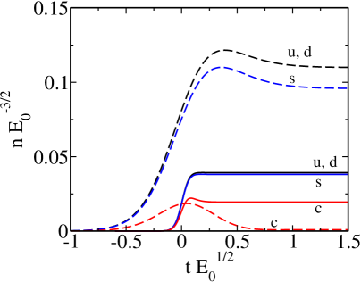
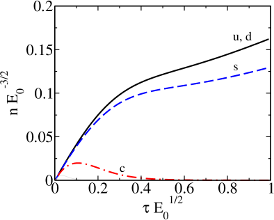
Figure 1: Left panel: the total quark-pair number densities for different flavours, $n_{i}(t)$, as a function of time $t$ for short pulse width $\tau E_{0}^{1/2}=0.1$ (solid lines) and long pulse width $\tau E_{0}^{1/2}=0.5$ (dashed lines). Right panel: the total quark-pair number densities at the final state, $n(t\gg\tau)$, as a function of pulse width $\tau$.

  

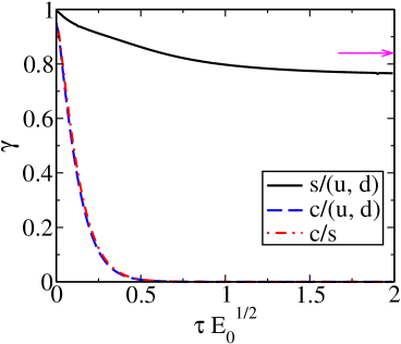
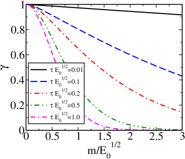
Figure 2: Left panel: the pulse width, $\tau$, dependence of the suppression factor $\gamma$. Arrow indicates the Schwinger limit for strangeness suppression factor. Right panel: the quark mass, $m$, dependence of the suppression factor $\gamma$ at different pulse width.

The ratio of number densities of heavy quark-pairs, e.g. strange, to light quark-pairs (u, d-quarks) is widely known as a suppression factor. In our model it is defined in the asymptotic future (c.f.  [11]), $t\gg\tau$, as

$$\gamma=\lim_{t\to\infty}n_{\rm heavy}(t)/n_{\rm light}(t),$$ (35)

where $n_{q}(t)$ is the number density of corresponding quark-pairs given by

$$n_{q}(t)=\nu\int\frac{d^{3}k}{(2\pi)^{3}}f_{q}(\bi{k},t)$$ (36)

with degeneracy factor $\nu=2({\rm spin})\times 2({\rm quark-antiquark})\times N_{c}({\rm color})$.

In Fig. 1 the time evolution of quark-pair number densities, $n_{i}$, are displayed for different pulse widths, $\tau E_{0}^{1/2}=0.1$ and 0.5. For short pulse width the quark-pair number densities are comparable with each other (solid lines). In this case the particle production happens during the whole evolution of the field. In contrast to this, for long pulse, the number densities of produced charm quark-pairs becomes negligible in the final state, because charm-pair production is balanced by subsequent absorption by the field. This dependence on the pulse width is also demonstrated on the right panel of Fig. 1. This figure clearly displays that charm quark-pair production is substantially enhanced in the cases of short pulse widths, and this enhancement has a maximum at $\tau\sim 0.1\sqrt{E_{0}}$. In opposite to the heavy charm quark, light and strange quark-pair productions are increasing with the pulse width, without any local maximum.

We have investigated the suppression factor and its dependence on pulse widths and quark masses. Fig. 2 summarizes our results. On the left panel the dependence on the pulse width is displayed. The strange to light ratio has a weak dependence on the pulse width, its value is approaching slowly the asymptotic value of Schwinger limit (0.84) from below, similarly to U(1) gauge field [6]. For charm quark this Schwinger limit is negligibly small, which value is reproduced by our numerical calculation for very long pulse width. On the other hand, at short pulse widths, the relative charm production is surprisingly large, which does not follow any earlier expectation. Considering charm to light and charm to strange ratios, only a slight difference can be seen between them. On the right panel we display the quark mass dependence of the suppression factor for different pulse widths. For short pulse width the suppression factor is decreasing almost linearly with increasing quark mass value. For large pulse widths we can see a very fast ($\sim\exp\{-m^{2}/E_{0}\}$) drop, which is consistent with the Schwinger formula.

5 Conclusion

We have calculated light, strange and charm quark-pair production in time-dependent SU(2) non-Abelian field. Applying a pulse-like time evolution and investigating the influence of pulse width, we observed that light and strange quark-pairs are produced as we expected, approaching the Schwinger limit. Charm quark-pairs followed this behaviour for large pulse widths. However, for short pulses we did not see the expected charm suppression, connected to the large charm quark mass. Indeed, the large value of inverse temporal width of the pulse, overwhelming the mass of the heavy quark, $1/\tau\gg m_{c}$, determines the quark-pair production. This finding could indicate the formation of collective gluon field via enhanced heavy quark-pair production at RHIC. The issue of quantitative calculation of particle suppression factors for different quarks and comparison with the existing models will be addressed elsewhere.

References

References

[1]
B. Andersson et al.,
Phys. Rep. 97 (1983) 31;
Nucl. Phys. B281 (1987) 289.
[2]
M. Gyulassy and L. McLerran,
Phys. Rev. C56 (1997) 2219.
[3]
V. Topor Pop, et al.
Phys. Rev. C72 (2005) 054901; arXiv:hep-ph/0608136; Phys. Rev. C 75, 014904 (2007).
[4]
V. V. Skokov and P. Lévai,
Phys. Rev. D51 (2005), 094010 [arXiv:hep-ph/0410339].
[5]
V. V. Skokov and P. Lévai,
Phys. Rev. D78 (2008) 054004 [arXiv:0710.0229].
[6]
A. V. Prozorkevich, et al.
Phys. Lett. B 583 (2004) 103 [arXiv:nucl-th/0401056].
[7]
T. Lappi, Phys. Rev. C67 (2003) 054903.
[8]
F. Gelis, K. Kajantie, and T. Lappi,
Phys. Rev. C71 (2005) 024904;
Phys. Rev. Lett. 96 (2006) 032304;
Eur. Phys. J. A29 (2006) 89.
[9]
A. V. Prozorkevich, S. A. Smolyansky, and S. V. Ilyin,
arXiv:hep-ph/0301169.
[10]
S. Ochs and U. Heinz,
Ann. Phys. 266 (1998) 351.