Quantum Non-Magnetic state near Metal-Insulator Transition - a Possible Candidate of Spin Liquid State

Abstract

In this paper, based on the formulation of O(3) non-linear $\sigma$ model, we study two dimensional $\pi-flux$ Hubbard model at half-filling. A quantum non-magnetic insulator is explored near metal-insulator transition that may be a possible candidate of spin liquid state. Such quantum non-magnetic insulator on square lattice is not induced by frustrations. Instead, it originates from quantum spin fluctuations with relatively small effective spin-moments. In the strong coupling limit, our results of spin velocity and spin order parameter agree with results obtained from earlier calculations.

PACS numbers: 71.10.Fd, 71.10.Hf, 75.10.-b, 71.30.+h

People have been seeking for quantum spin liquid states in spin models with predominantly antiferromagnetic short ranged interactions for over two decades Fazekas . For example, various approaches show that quantum spin liquids may exist in two-dimensional (2D) $S=1/2$ J₁-J₂ model or Heisenberg model on Kagomé lattice. In these models, the quantum spin liquids are accessed (in principle) by appropriate frustrating interactions. In particular, such type of spin liquid states can be described by the Hubbard model formalism in the strong coupling limit.

Recent experiments on the triangular lattice show that the spin liquid ground state may be realized in the organic material $\mathrm{\kappa-(BEDT-TTF)}_{2}\mathrm{CU}_{2}\mathrm{(CN)}_{3}$Shimizu ; Kawamoto ; Kurosaki . Motivated by experiments, $U(1)$ slave-rotor theory of Hubbard model on triangular latticeLee and its $SU(2)$ generalization on honeycomb lattice were formulatedHermele . It is predicted that quantum spin liquids may lie in the insulating side of the metal-insulator (MI) transitions. Because the spin liquid is adjacent to the MI transitions, people may guess it is the local charge fluctuations rather than frustrations that disrupt spin ordering and drive the ground state to a spin liquid. Such type of spin liquid can be described by the Hubbard model formalism of the intermediate coupling region.

Recently, it becomes hot to use ultracold atoms as simulators of quantum many-body systemsBloch's review . In particular, the $\pi$-flux Hubbard model (or the Hubbard model with $\phi$ flux) on square lattice has been designed with ultracold atoms in an optical lattice. An artificial magnetic field of $\pi$-flux (or $\phi$ flux) in an optical square lattice is proposed to be realized by different approaches, such as laser assisted tunneling method2 , laser methods by employing dark states1 or dressing two-photon by laser fields3 . Without the nesting condition, the MI transition of the $\pi$-flux Hubbard model may differ from that of the traditional Hubbard model on square lattice. Thus, due to nodal fermions in the non-interacting limit, it becomes an interesting issue to learn the MI transition of the $\pi$-flux Hubbard model. In addition, it is known that the insulator state of the $\pi$-flux Hubbard model belongs to a special class of antiferromagnetic (AF) ordered state - nodal AF insulator (NAI), an AF order with relativistic massive fermionic excitationskou . Another issue here is whether the nodal AF insulator is a long range AF order or a short range one.

In the followings an O(3) non-linear $\sigma$ model ($\mathrm{NL}\sigma\mathrm{M}$) is developed to investigate properties of NAI in the $\pi$-flux Hubbard model. Based on the $\mathrm{NL}\sigma\mathrm{M,}$ we will show that a non-magnetic insulator (a short range AF order) may exist in the NAI of 2D $\pi$-flux Hubbard model when the spin fluctuations are considered.

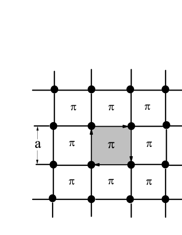
Figure 1: Illustrations of a $\pi$-flux lattice. There is a $\pi$-flux phase when an atom hops aroud a plaquette (the gray rectangle). Where $a$ is the length of the side that is chosen to be unit.

Metal-Insulator transitions of the $\pi$-flux Hubbard model - The Hamiltonian of 2D $\pi$-flux Hubbard model is

$$\mathcal{H}=-\sum\limits_{\langle i,j\rangle}\left(t_{ij}\hat{c}_{i}^{\dagger}\hat{c}_{j}+h.c.\right)+U\sum_{i}\hat{n}_{i\uparrow}\hat{n}_{i\downarrow}-\mu\sum\limits_{i}\hat{c}_{i}^{\dagger}\hat{c}_{i}.$$ (1)

Here $\hat{c}_{i}=(\hat{c}_{i\uparrow},\hat{c}_{i\downarrow})^{T}$ are defined as electronic annihilation operators. $U$ is the on-site Coulomb repulsion. $\mu$ is the chemical potential and at half-filling it is $\frac{U}{2}$. $\langle i,j\rangle$ denotes two sites on a nearest-neighbor link. $\hat{n}_{i\uparrow}$ and $\hat{n}_{i\downarrow}$ are the number operators of electrons at site $i$ with up-spin and down spin, respectively. There is a $\pi$-flux phase when an atom hops around a plaquette in a $\pi$-flux lattice(See Fig.1). So the nearest neighbor hopping $t_{i,j}$ in a $\pi$-flux lattice could be chosen ashsu $t_{i,i+\hat{x}}=t,t_{i,i+\hat{y}}=te^{\pm i\frac{\pi}{2}}.$

Figure 2: The staggered magnetization of the $\pi$-flux Hubbard model (circle solid line) and that of the traditional Hubbard model (square solid line) at zero temperature. $\left(U/t\right)_{c1}\simeq 3.11$ is the critical point of the metal-insulator(MI) transition of the $\pi$-flux Hubbard model.

Because the Hubbard model on bipartite lattices is unstable against antiferromagnetic (AF) instability, at half-filling, the ground state may be an insulator with AF order (NAI). Such AF order is described by the following mean field result

$$\langle\hat{c}_{i,\sigma}^{{\dagger}}\hat{c}_{i,\sigma}\rangle=\frac{1}{2}\left(1+(-1)^{i}\sigma M\right)$$ (2)

Here $M$ is the staggered magnetization. For the cases of spin up and spin down, we have $\sigma=+1$ and $\sigma=-1$, respectively. Then in the mean field theory, the Hamiltonian of the 2D $\pi$-flux Hubbard model is obtained as

$$\mathcal{H}=-\sum\limits_{\left\langle ij\right\rangle}(t_{i,j}\hat{c}_{i}^{\dagger}\hat{c}_{j}+h.c.)-\sum_{i}\left(-1\right)^{i}\Delta\hat{c}_{i}^{\dagger}\mathbf{\sigma}_{z}\hat{c}_{i}$$ (3)

where $\Delta=\frac{UM}{2}$ leads to the energy gap of electrons and $\sigma_{z}$ is the Pauli matrix. After diagonalization, the spectrum of the electrons is obtained as

$$E_{\mathbf{k}}=\pm\sqrt{\left|\xi_{\mathbf{k}}\right|^{2}+\Delta^{2}}$$ (4)

where $\left|\xi_{\mathbf{k}}\right|=\sqrt{4t^{2}\left(\cos^{2}k_{x}+\cos^{2}k_{y}\right)}$ corresponds to the energy of free fermions. By minimizing the free energy at temperature $T$ in the Brillouin zone, the self-consistent equation of (3) is reduced into

$$\frac{1}{N}\sum\limits_{\mathbf{k}}\frac{U}{2E_{\mathbf{k}}}\tanh(\frac{E_{\mathbf{k}}}{2k_{B}T})=1$$ (5)

where $N$ is the number of the particles.

It is well known that due to the nesting effect, there is no MI transition of the traditional Hubbard model (arbitrary interaction will lead to a magnetic instability). The situation is difference for the MI transition of $\pi$-flux Hubbard model. The MI transition of the $\pi$-flux Hubbard model occurs at a critical value about $U/t\simeq 3.11$hsu (See Fig.2). In the weakly coupling limit $\left(U/t<3.11\right)$, the ground state is a semi-metal (SM) with nodal fermi-pointskou . In the strong coupling region $\left(U/t>3.11\right)$, due to $M\neq 0$, the ground state becomes an insulator with massive fermionic excitations. By contrast, there is only the insulating phase of the traditional Hubbard model (See Fig.2). However, the non-zero value of $M$ only means the existence of effective spin moments. It does not necessarily imply that the ground state of NAI is a long range AF order because the direction of the spins is chosen to be fixed along $\mathbf{\hat{z}}$-axis in the mean field theory. Thus one needs to examine stability of magnetic order against quantum fluctuations of effective spin moments based on a formulation by keeping spin rotation symmetry.

Effective nonlinear $\sigma$ model of spin fluctuations - In the following parts we will focus on the NAI state and don’t consider local charge fluctuations and the amplitude fluctuations of $M$ that are all gapped in the region of $M\neq 0$com1 . To deal with the spin fluctuations, we use the path-integral formulation of electrons with spin rotation symmetrywen ; dup ; dupuis ; Schulz ; weng . The interaction term in Eq.(1) can be handled by using the SU(2) invariant Hubbard-Stratonovich decomposition in the arbitrary on-site unit vector $\mathbf{\Omega}_{i}$

$$\hat{n}_{i\uparrow}\hat{n}_{i\downarrow}=\frac{\left(\hat{c}_{i}^{\dagger}\hat{c}_{i}\right)^{2}}{4}-\frac{1}{4}[\mathbf{\Omega}_{i}\mathbf{\cdot}\hat{c}_{i}^{{\dagger}}\mathbf{\sigma}\hat{c}_{i}]^{2}$$ (6)

Here $\mathbf{\sigma=}\left(\sigma_{x},\sigma_{y},\sigma_{z}\right)$ are the Pauli matrices. By replacing the electronic operators $\hat{c}_{i}^{\dagger}$ and $\hat{c}_{j}$ by Grassmann variables $c_{i}^{\ast}$ and $c_{j}$, the effective Lagrangian of the 2D $\pi$-flux Hubbard model at half filling is obtained:

$$\mathcal{L}_{\mathrm{eff}}=\sum_{i}c_{i}^{\ast}\partial_{\tau}c_{i}-\sum\limits_{\left\langle ij\right\rangle}\left(t_{i,j}c_{i}^{\ast}c_{j}+h.c.\right)-\Delta\sum_{i}c_{i}^{\ast}\mathbf{\Omega}_{i}\mathbf{\cdot\sigma}c_{i}.$$ (7)

In particular, we describe the vector $\mathbf{\Omega}_{i}$ with the haldane’s mapping:

$$\mathbf{\Omega}_{i}=(-1)^{i}\mathbf{n}_{i}\sqrt{1-\mathbf{L}_{i}^{2}}+\mathbf{L}_{i}.$$ (8)

Here $\mathbf{n}_{i}=(n_{i}^{x},n_{i}^{y},n_{i}^{z})$ is the Néel vector with $\mathbf{n}_{i}^{2}=1$ and $\mathbf{L}_{i}$ is the small transverse canting field with $\mathbf{L}_{i}\cdot$ $\mathbf{n}_{i}=0$dupuis ; Haldane ; Auerbach .

Then we rotate $\mathbf{n}_{i}$ to $\mathbf{\hat{z}}$-axis at each site on both sublattices by performing the following spin transformationwen ; dup ; dupuis ; Schulz ; weng , $\psi_{i}=U_{i}c_{i},$ $U_{i}^{\dagger}\mathbf{n}_{i}\cdot\mathbf{\sigma}U_{i}=\mathbf{\sigma}_{z}$ and $U_{i}^{\dagger}\mathbf{L}_{i}\cdot\mathbf{\sigma}U_{i}=\mathbf{l}_{i}\cdot\mathbf{\sigma.}$ After the spin transformation, the effective Hamiltonian becomes:

$$\mathcal{H}_{\mathrm{eff}}=\sum\limits_{i}\psi_{i}^{\ast}a_{0}\left(i\right)\psi_{i}-\sum\limits_{<ij>}(t_{i,j}\psi_{i}^{\ast}e^{ia_{ij}}\psi_{j}+h.c.)-\Delta\sum\limits_{i}\psi_{i}^{\ast}[(-1)^{i}\mathbf{\sigma}_{z}\sqrt{1-\mathbf{l}_{i}^{2}}+\mathbf{l}_{i}\cdot\mathbf{\sigma]}\psi_{i}$$ (9)

where the auxiliary gauge fields $a_{ij}=a_{ij,1}\sigma_{x}+a_{ij,2}\sigma_{y}$ and $a_{0}\left(i\right)=a_{0,1}\left(i\right)\sigma_{x}+a_{0,2}\left(i\right)\sigma_{y}\$are defined by $e^{ia_{ij}}=U_{i}^{\dagger}U_{j}$ and $a_{0}\left(i\right)=U_{i}^{\dagger}\partial_{\tau}U_{i}.$ In terms of the mean field result, $M=\left(-1\right)^{i}\langle\psi_{i}^{\ast}\mathbf{\sigma}_{z}\psi_{i}\rangle,$ we obtain the effective Hamiltonian:

$$\mathcal{H}_{\mathrm{eff}} \simeq \sum\limits_{i}\psi_{i}^{\ast}[a_{0}\left(i\right)-\Delta\mathbf{\sigma\cdot\mathbf{l}_{i}}]\psi_{i}-\Delta\sum\limits_{i}(-1)^{i}\psi_{i}^{\ast}\sigma_{z}\psi_{i}-\sum\limits_{\left\langle ij\right\rangle}[t_{i,j}\psi_{i}^{\ast}(1+ia_{ij})\psi_{j}+h.c.]+\Delta M\sum\limits_{i}\frac{\mathbf{l}_{i}^{2}}{2}$$ (10)

In this equation we have used the approximations $\sqrt{1-\mathbf{l}_{i}^{2}}\simeq 1-\frac{\mathbf{l}_{i}^{2}}{2}$ and $e^{ia_{ij}}\simeq 1+ia_{ij}$.

In the next step, we integrate the gapped fermion fields and get the quadric terms of $[a_{0}\left(i\right)-\Delta\mathbf{\sigma\cdot l}_{i}]$ and $a_{ij}$. Then the effective action becomes:

$$\mathcal{S}_{\mathrm{eff}}=\frac{1}{2}\int_{0}^{\beta}d\tau\sum_{i}[-4\varsigma(a_{0}\left(i\right)-\Delta\mathbf{\sigma\cdot l}_{i})^{2}+4\rho_{s}a_{ij}^{2}+\frac{2\Delta^{2}}{U}\mathbf{l}_{i}^{2}]$$ (11)

where the parameters $\rho_{s}$ and $\varsigma$ are derived from the following two equationsdet :

$$\rho_{s} = \frac{1}{N}\sum\limits_{\mathbf{k}}\frac{\epsilon^{2}}{2(\left|\xi_{\mathbf{k}}\right|^{2}+\Delta^{2})^{\frac{3}{2}}},$$ (12)

$$\varsigma = \frac{1}{N}\sum\limits_{\mathbf{k}}\frac{\Delta^{2}}{4(\left|\xi_{\mathbf{k}}\right|^{2}+\Delta^{2})^{\frac{3}{2}}}.$$ (13)

and the corresponding coefficient $\epsilon^{2}$ is given as:

$$\epsilon^{2}=t^{2}[\cos\left(2k_{x}\right)\left(\Delta^{2}+8t^{2}+4t^{2}\cos\left(2k_{y}\right)\right)+\Delta^{2}+3t^{2}+t^{2}\cos\left(4k_{x}\right)]$$ (14)

To learn the properties of the low energy physics, we study the continuum theory of the effective action in Eq.(11). In the continuum limit, we denote $\mathbf{n}_{i}$, $\mathbf{l}_{i}$, $ia_{ij}\simeq U_{i}^{\dagger}U_{j}-1$ and $a_{0}\left(i\right)=U_{i}^{\dagger}\partial_{\tau}U_{i}$ by $\mathbf{n}(x,y)$, $\mathbf{l}(x,y)$, $U^{\dagger}\partial_{x}U$ (or $U^{\dagger}\partial_{y}U$) and $U^{\dagger}\partial_{\tau}U,$ respectively. From the relations between $U^{\dagger}\partial_{\mu}U$ and $\partial_{\mu}\mathbf{n,}$

$$a_{\tau}^{2} = a_{\tau,1}^{2}+a_{\tau,2}^{2}=-\frac{1}{4}(\partial_{\tau}\mathbf{n})^{2},\text{ }\tau=0,$$ (15)

$$a_{\mu}^{2} = a_{\mu,1}^{2}+a_{\mu,2}^{2}=\frac{1}{4}(\partial_{\mu}\mathbf{n})^{2},\text{ }\mu=x,y,$$ (16)

$$\mathbf{a}_{0}\mathbf{\cdot l} \mathbf{=} \mathbf{-}\frac{i}{2}\left(\mathbf{n}\times\partial_{\tau}\mathbf{n}\right)\cdot\mathbf{l,}$$ (17)

the continuum formulation of the action in Eq.(11) turns into

$$\mathcal{S}_{\mathrm{eff}}=\frac{1}{2}\int_{0}^{\beta}d\tau\int d^{2}\mathbf{r}[\varsigma(\partial_{\tau}\mathbf{n)}^{2}+\rho_{s}\left(\mathbf{\bigtriangledown n}\right)^{2}-4i\Delta\varsigma\left(\mathbf{n}\times\partial_{\tau}\mathbf{n}\right)\cdot\mathbf{l}+(\frac{2\Delta^{2}}{U}-4\Delta^{2}\varsigma)\mathbf{l}^{2}]$$ (18)

where the vector $\mathbf{a}_{0}$ is defined as $\left(a_{0,1},a_{0,2},0\right).$

Finally we integrate the transverse canting field $\mathbf{l}$ and obtain the effective $\mathrm{NL}\sigma\mathrm{M}$ of the $\pi$-flux Hubbard model as

$$\mathcal{S}_{\mathrm{eff}}=\frac{1}{2g}\int_{0}^{\beta}d\tau\int d^{2}r[\frac{1}{c}\left(\partial_{\tau}\mathbf{n}\right)^{2}+c\left(\mathbf{\bigtriangledown n}\right)^{2}]\text{ }$$ (19)

with a constraint $\mathbf{n}^{2}=1.$ The coupling constant $g$ and spin wave velocity $c$ are defined as

Figure 3: The spin stiffness $\rho_{s}$ and the spin wave velocity $c$ of the $\pi$-flux Hubbard model.

$$g = \frac{c}{\rho_{s}}$$ (20)

$$c^{2} = \frac{\rho_{s}}{\chi^{\perp}}$$ (21)

Here $\rho_{s}$ is the spin stiffness and $\chi^{\perp}=(\frac{1}{\varsigma}-2U)^{-1}$ is the transverse spin susceptibility.

The numerical results of $\rho_{s}$ and $c$ of the $\pi$-flux Hubbard model are illustrated in Fig.3, where one can find that $\rho_{s}=0.03936t=0.2460J$, $c=0.226278t=1.41424J$ in the strong coupling limit$\left(U=25t\right)$ match the earlier results $\rho_{s}=\frac{J}{4},$ $c=\sqrt{2}J$ ($J=\frac{4t^{2}}{U}$) that are obtained from the Heisenberg model Schrieffer ; Singh ; Chubukov ; man .

In addition, we need to determine another important parameter - the cutoff $\Lambda$. On the one hand, the effective $\mathrm{NL}\sigma\mathrm{M}$ is valid within the energy scale of Mott gap, $2\Delta=UM.$ On the other hand, the lattice constant is a natural cutoff. Thus the cutoff is defined as the following equation $\Lambda=\min(1,\frac{2\Delta}{c})$dupuis .

Magnetic properties of the nodal AF insulator : In this section we will use the effective $\mathrm{NL}\sigma\mathrm{M}$ to study the magnetic properties of the insulator state. The Lagrangian of $\mathrm{NL}\sigma\mathrm{M}$ with a constraint ($\mathbf{n}^{2}=1$) by a Lagrange multiplier $\lambda$ becomes

$$\mathcal{L}_{\mathrm{eff}}=\frac{1}{2cg}\left[\left(\partial_{\tau}\mathbf{n}\right)^{2}+c^{2}\left(\mathbf{\bigtriangledown n}\right)^{2}+i\lambda(1-\mathbf{n}^{2})\right]$$ (22)

where $i\lambda=m^{2}$ and $m$ is the mass gap of the spin fluctuations.

At finite temperature, by rescaling the field $n\rightarrow\sqrt{N}n$ and using the large-N approximation, the solution of $n_{0}=\left\langle\mathbf{n}\right\rangle$ is always zero that is consistent to the Mermin-Wigner theorem. From Eq.(22), we may get the solution of $m$ as

$$m=2T\sinh^{-1}[e^{-\frac{2\pi c}{gT}}\sinh(\frac{c\Lambda}{2k_{\mathrm{B}}T})].$$ (23)

Figure 4: The dimensionless coupling constant $\alpha$ of the $\pi$-flux Hubbard model (cicle solid line) and that of the traditional Hubbard model (square solid line). There are three regimes, semimetal(SM), quantum disordered(QD), antiferromagnetic(AF), separated by two critical points $\left(U/t\right)_{c1}\simeq 3.11$, $\left(U/t\right)_{c2}\simeq 4.26,$ respectively. There is only the AF regime on the traditional square lattice.

At zero temperature, the solutions of $n_{0}$ and $m$ of Eq.(22) are determined by the dimensionless coupling constant $\alpha=g\Lambda.$ In particular, there exists a critical point $\alpha_{c}=4\pi$ $($ or $g_{c}=\frac{4\pi}{\Lambda})$ : For the case of $\alpha<4\pi,$ we get solutions of $n_{0}$ and $m$ as $n_{0}=(1-\frac{g}{g_{c}})^{1/2}$ and $m=0$. For the case of $\alpha>4\pi,$ we get solutions of $n_{0}$ and $m$ as $n_{0}=0$ and $m=4\pi c(\frac{1}{g_{c}}-\frac{1}{g})$. So we calculate the dimensionless coupling constant $\alpha=g\Lambda$ of the $\pi$-flux Hubbard model and show results in Fig.4. The quantum critical point corresponding to $\alpha_{c}=4\pi$ turns into $U/t\simeq 4.26$ which devides the NAI state into two phases - a quantum disordered state (QD) in the region of $3.11<U/t<4.26$ and a long range AF order in the region of $U/t>4.26$. The results show sharp contrast to those from the traditional Hubbard model, where the dimensionless coupling constant is always smaller than $\alpha_{c}=4\pi$.

In the region of $U/t>4.26$ (where $\alpha<\alpha_{c}$), at low temperature the mass gap $m$ of spin fluctuations is determined by

$$m\simeq 2k_{\mathrm{B}}T\exp[-\frac{2\pi c}{k_{\mathrm{B}}T}(\frac{1}{g}-\frac{1}{g_{c}})].$$ (24)

Because the energy scale of the mass gap $m$ is always much smaller than the temperature, i.e., $m\ll k_{\mathrm{B}}T$ (or $\omega_{n}$), quantum fluctuations become negligible in a sufficiently long wavelength and low energy regime $\left(m<\left|c\mathbf{q}\right|<k_{\mathrm{B}}T\right).$ Thus in this region one may only consider the purely static (semiclassical) fluctuations. The effective Lagrangian of the NL$\sigma$M then becomes

$$\mathcal{L}=\frac{\tilde{\rho}_{s}}{2}\left(\mathbf{\bigtriangledown n}\right)^{2}$$ (25)

where $\tilde{\rho}_{s}=c\left(\frac{1}{g}-\frac{1}{g_{c}}\right)$ is the renomalized spin stiffness. At zero temperature, the mass gap vanishes (See Fig.5(a)) which means that long range AF order appears. To describe the long range AF order, we introduce a spin order parametercha ; chu ; sech

$$\mathcal{M}_{0}=\frac{M}{2}n_{0}=\frac{M}{2}(1-\frac{g}{g_{c}})^{1/2}$$ (26)

As shown in Fig.5(b), the ground state of long range AF ordered phase has a finite spin order parameter. In addition, in the strong coupling limit, $U/t\rightarrow\infty$, the values naturally match the results derived from the Heisenberg model mapped from the $\pi$-flux Hubbard model.

Figure 5: The mass gap $m$ of the spin fluctuations and the ordered spin moment $\mathcal{M}_{0}$ of the $\pi$-flux Hubbard model at zero temperature. There are three regimes, semimetal(SM), quantum disordered(QD), antiferromagnetic(AF), separated by two critical points $\left(U/t\right)_{c1}\simeq 3.11$, $\left(U/t\right)_{c2}\simeq 4.26,$ respectively.

In the region of $3.11<U/t<4.26$ $($where $\alpha>\alpha_{c}),$ there is a finite mass gap of spin fluctuations, $m=4\pi c(\frac{1}{g_{c}}-\frac{1}{g})$ at zero temperature (See Fig.5(a)). Therefore, the ground state of the insulator in this region is not a long range AF order. Instead, it is a quantum disordered state (or non-magnetic insulator state) with zero spin order parameter $\mathcal{M}_{0}=0$ (See Fig.5(b)). The existence of a non-magnetic insulator state provides an alternative candidate for finding spin liquid state.

Obviously, such type of quantum non-magnetic insulator on bipartite lattices is induced neither by geometry frustrations regarded as the examples in varied spin models nor by the local charge fluctuations with finite energy gap. What is the physics origin of this quantum non-magnetic state? The key point is that, due to the special electron dispersion (the existence of nodal fermions for non-interacting case) the coupling constant $g$ is almost proportional to $\frac{1}{M}$ near the MI transition (See Fig.6). Hence the non-magnetic state originates from quantum spin fluctuations of relatively small effective spin-moments, $M\rightarrow 0$.

Figure 6: Illustrations of the relations between the coupling constant $g$ and the staggered magnetization $M$ of the $\pi$-flux Hubbard model(cicle solid line) and the traditional Hubbard model (square solid line in inset (b)).

Let us compare the properties of the insulator state in $\pi$-flux Hubbard model and those in the traditional Hubbard model. For the traditional Hubbard model on square lattice, due to the nesting effect, there is no MI transition at finite $U$ and the insulator state here doesn’t belong to NAI. In the $U/t\rightarrow 0$ limit, the coupling constant $g$ is not proportional to $\frac{1}{M}$(See Fig.6). Instead, $g$ is about $g\sim\frac{2}{\sqrt{\pi}}(\frac{U}{t})^{1/4}$ that becomes smaller and turns into zero the weakly coupling limit(See more details in Ref.dupuis ). So the quantum fluctuations of the effective spin-moments are suppressed. Using the NL$\sigma$M formulation, due to $g<g_{c}$ (See Fig.4), the ground state of the Hubbard model on square lattice always has a long range AF order.

Conclusion - In this paper, to deal with the spin fluctuations, we use the path-integral formulation of electrons with spin rotation symmetry and then the effective $\mathrm{NL}\sigma\mathrm{M}$ is obtained to describe the NAI state of the $\pi$-flux Hubbard model. We calculate the spin stiffness, the transverse spin susceptibility, the spin wave velocity and the coupling constant $g$. In the strong coupling limit ($U/t\rightarrow\infty$), our results of spin velocity and spin order parameter agree with the results obtained from earlier calculations of the traditional Hubbard model. However, we find that the coupling constant $g$ in the NAI state of the $\pi$-flux Hubbard model shows different behaviors to that in the insulator state of the traditional Hubbard model. In particular, a quantum non-magnetic insulator state $\left(3.11<U/t<4.26\right)$ is explored near the MI transition that corresponds to the strong coupling region of the effective $\mathrm{NL}\sigma\mathrm{M,}$ $g>g_{c}$. Such type of quantum non-magnetic insulator in bipartite lattices is driven by quantum spin fluctuations of relatively small effective spin-moments.

Such non-magnetic insulator state is different from that proposed in organic material $\mathrm{\kappa-(BEDT-TTF)}_{2}\mathrm{CU}_{2}\mathrm{(CN)}_{3}$ by $U(1)$ slave-rotor theory in Ref.Lee . Firstly, the non-magnetic insulator state is really a short range AF insulator (although we don’t know its exact nature) followed by a long range AF order with increasing $U;$ however, the spin liquid state in Ref.Lee is really a $U(1)$ spin liquid with spinon fermi surface, of which no long range AF order appears with increasing $U$. Secondly, the local charge fluctuations play important role in the slave-rotor theory; in contrast, the local charge fluctuations are irrelevant here. Therefore, our results illustrate a new candidate for finding spin liquid state.

An interesting issue is the nature of the non-magnetic insulator. Is it a valence-band crystal read , or algebra spin liquid statewen ; wen1 , …? In addition, another issue is whether there exists non-magnetic insulator state of the Hubbard model in honeycomb lattice, of which there also exist nodal fermions. These issues are beyond the scope of the present work and will be left for a future study.

The authors acknowledge stimulating discussions with Z.Y. Weng, T. Li, N.H. Tong, F. Yang, P. Ye. This research is supported by NCET, NFSC Grant no. 10574014, 10874017.

References

- (1) P. Fazekas and P.W. Anderson, Philos. Mag. 30, 432 (1974); P. W. Anderson, Science 235, 1196 (1987).
- (2) Y. Shimizu, et al., Phys. Rev. Lett. 91, 107001 (2003).
- (3) A. Kawamoto, Y. Honma, and K. I. Kumagai, Phys. Rev. B 70, 060510(R) (2004).
- (4) Y. Kurosaki, et al., Phys. Rev. Lett. 95, 177001 (2005).
- (5) S. S. Lee and P. A. Lee, Phys. Rev. Lett. 95, 036403 (2005).
- (6) Michael Hermele, Phys. Rev. B 76, 035125 (2007).
- (7) I. Bloch, et. al. Rev. Mod. Phys. 80, 885 (2008).
- (8) D. Jaksch and P. Zoller, New J. Phys. 5, 56 (2003).
- (9) G. Juzeliūnas and P. Öhberg, Phys. Rev. Lett. 93, 033602 (2004); G. Juzeliūnas, P. Öhberg, J. Ruseckas and A. Klein, Phys. Rev. A 71 , 053614 (2005).
- (10) Y. J. Lin, et. al., Phys. Rev. Lett. 102, 130401 (2009).
- (11) S. P. Kou, Phys. Rev. B 78, 233104 (2008).
- (12) T. C. Hsu, Phys. Rev. B 41, 11379 (1990).
- (13) When the mean field value of almost vanishes, approaching the critical point (), due to the strong charge fluctuations and the strong amplitude fluctuations of , cannot be used and our results cannot be reliable.
- (14) N. Dupuis, Phys. Rev. B 65, 245118 (2002).
- (15) K. Borejsza, N. Dupuis, Euro Phys. Lett. 63, 722 (2003); K. Borejsza and N. Dupuis Phys. Rev. B 69, 085119 (2004).
- (16) X. G. Wen, Quantum Field Theory of Many-Body Systems, (Oxford Univ. Press, Oxford, 2004).
- (17) H. J. Schulz, Phys. Rev. Lett. 65, 2462(1990); H. J. Schulz, in The hubbard Model, edited by D. Baeriswyl(Plenum, New York, 1995).
- (18) Z. Y. Weng, C. S. Ting, and T. K. Lee, Phys. Rev. B 43, 3790 (1991).
- (19) F.D.M. Haldane, Phys. Lett. 93A, 464(1983).
- (20) A. Auerbach, Interacting Electrons and Quantum Magnetism (Springer-Verlag, New York, 1994).
- (21) See the detailed calculation in Refs. dupuis and wen .
- (22) J.R. Schrieffer, X.G. Wen, and S.C. Zhang, Phys. Rev. B 39, 11663 (1989).
- (23) A. Singh and Z. Tesanovic, Phys. Rev. B 41, 614 (1990).
- (24) A. V. Chubukov and D.M. Frenkel, Phys. Rev. B 46, 11884 (1992)
- (25) E. Manousakis, Rev. Mod. Phys. 63, 1 (1991)
- (26) S. Chakravarty, et al., Phys. Rev. B 39, 2344 (1989).
- (27) A. V. Chubukov and S. Sachdev, J. Ye, Phys. Rev. B 49, 11919 (1994)
- (28) S. Sachdev, Quantum Phase Transitions, (Cambridge University Press, 1999).
- (29) N. Read and S. Sachdev, Phys. Rev. Lett. 62, 1694 (1989); Phys. Rev. B 42, 4568 (1990); N. Read and S. Sachdev, Phys. Rev. Lett. 66, 1773 (1991).
- (30) X. G. Wen, Phys. Rev. B 65, 165113 (2002).