Post Common Envelope Binaries from SDSS. V: Four eclipsing white dwarf main sequence binaries

Abstract

We identify SDSS 011009.09+132616.1, SDSS 030308.35+005444.1, SDSS 143547.87+373338.5 and SDSS 154846.00+405728.8 as four eclipsing white dwarf plus main sequence (WDMS) binaries from the Sloan Digital Sky Survey, and report on follow-up observations of these systems. SDSS 0110+1326, SDSS 1435+3733 and SDSS 1548+4057 contain DA white dwarfs, while SDSS 0303+0054 contains a cool DC white dwarf. Orbital periods and ephemerides have been established from multi-season photometry. SDSS 1435+3733, with $\mbox{$P_{\mathrm{orb}}$}=3$ h has the shortest orbital period of all known eclipsing WDMS binaries. As for the other systems, SDSS 0110+1326 has $\mbox{$P_{\mathrm{orb}}$}=8$ h, SDSS 0303+0054 has $\mbox{$P_{\mathrm{orb}}$}=3.2$ h and SDSS 1548+4057 has $\mbox{$P_{\mathrm{orb}}$}=4.4$ h. Time-resolved spectroscopic observations have been obtained and the H$\alpha$ and Ca II $\lambda\lambda$ 8498.02,8542.09,8662.14 triplet emission lines, as well as the Na I $\lambda\lambda$ 8183.27,8194.81 absorption doublet were used to measure the radial velocities of the secondary stars in all four systems. A spectral decomposition/fitting technique was then employed to isolate the contribution of each of the components to the total spectrum, and to determine the white dwarf effective temperatures and surface gravities, as well as the spectral types of the companion stars. We used a light curve modelling code for close binary systems to fit the eclipse profiles and the ellipsoidal modulation/reflection effect in the light curves, to further constrain the masses and radii of the components in all systems. All three DA white dwarfs have masses of $\mbox{$M_{\mathrm{WD}}$}\sim 0.4-0.6\,\mbox{$\mathrm{M}_{\odot}$}$, in line with the expectations from close binary evolution. The DC white dwarf in SDSS 0303+0054 has a mass of $\mbox{$M_{\mathrm{WD}}$}\ga 0.85\,\mbox{$\mathrm{M}_{\odot}$}$, making it unusually massive for a post-common envelope system. The companion stars in all four systems are M-dwarfs of spectral type M4 and later. Our new additions raise the number of known eclipsing WDMS binaries to fourteen, and we find that the average white dwarf mass in this sample is $<\mbox{$M_{\mathrm{WD}}$}>=0.57\pm 0.16\,\mbox{$\mathrm{M}_{\odot}$}$, only slightly lower than the average mass of single white dwarfs. The majority of all eclipsing WDMS binaries contain low-mass ($<0.6\,\mbox{$\mathrm{M}_{\odot}$}$) secondary stars, and will eventually provide valuable observational input for the calibration of the mass-radius relations of low-mass main sequence stars and of white dwarfs.

1 Introduction

White dwarfs and low-mass stars represent the most common types of stellar remnant and main sequence star, respectively, encountered in our Galaxy. Yet, despite being very common, very few white dwarfs and low mass stars have accurately determined radii and masses. Consequently, the finite temperature mass-radius relation of white dwarfs (e.g. Wood, 1995; Panei et al., 2000) remains largely untested by observations (Provencal et al., 1998). In the case of low mass stars, the empirical measurements consistently result in radii up to 15% larger and effective temperatures 400 K or more below the values predicted by theory (e.g. Ribas, 2006; López-Morales, 2007). This is most clearly demonstrated using low-mass eclipsing binary stars (Bayless & Orosz, 2006), but is also present in field stars (Berger et al., 2006; Morales et al., 2008) and the host stars of transiting extra-solar planets (Torres, 2007).

Eclipsing binaries are the key to determine accurate stellar masses and radii (e.g. Andersen, 1991; Southworth & Clausen, 2007). However, because of their intrinsic faintness, very few binaries containing white dwarfs and/or low mass stars are currently known. Here, we report the first results of a programme aimed at the identification of eclipsing white dwarf plus main sequence (WDMS) binaries, which will provide accurate empirical masses and radii for both types of stars. Because short-period WDMS binaries underwent common envelope evolution, they are expected to contain a wide range of white dwarf masses, which will be important for populating the empirical white dwarf mass-radius relation. Eclipsing WDMS binaries will also be of key importance in filling in the mass-radius relation of low-mass stars at masses $\la 0.6\,\mbox{$\mathrm{M}_{\odot}$}$.

The structure of the paper is as follows. The target selection for this programme is described in Sect. 2. In Sect. 3 we present our observations and data reduction in detail. We determine the orbital periods and ephemerides of the four eclipsing WDMS binaries in Sect. 4, and measure the radial velocities of the secondary stars in Sect. 5. In Sect. 6 we derive initial estimates of the stellar parameters from fitting the SDSS spectroscopy of our targets. Basic equations for the following analysis are outlined in Sect. 7. In Sect. 8 we describe our fits to the observed light curves, and present our results in Sect. 9. The past and future evolution of the four stars is explored in Sect. 10. Finally, we discuss and summarise our findings, including an outlook on future work in Sect. 11.

2 Target selection

We have selected eclipsing SDSS WDMS binaries based on the available information on the radial velocities of their companion stars, and/or evidence of a strong reflection effect.

Initially, we used SDSS spectroscopy to measure the radial velocity of the companion star either from the Na I $\lambda\lambda$ 8183.27,8194.81 absorption doublet, or from the H$\alpha$ emission line (see Rebassa-Mansergas et al. 2007 for details). SDSS J030308.35+005444.1 (henceforth SDSS 0303+0054) and SDSS J143547.87+373338.6 (henceforth SDSS 1435+3733) exhibited the largest secondary star radial velocities among $\sim 1150$ WDMS binaries which have SDSS spectra of sufficiently good quality, 287 $\mathrm{km\,s^{-1}}$ and 335 $\mathrm{km\,s^{-1}}$, respectively. For SDSS J011009.09+132616.1 (henceforth SDSS 0110+1326) two SDSS spectra are available, which differ substantially in the strength of the emission lines from the heated companion star. Photometric time series (Sect. 3) revealed white dwarf eclipses in all three objects. SDSS 1435+3733 has been independently identified as an eclipsing WDMS binary by Steinfadt et al. (2008).

As the number of SDSS WDMS binaries with known orbital periods, $P_{\mathrm{orb}}$, and radial velocity amplitudes, $K_{\mathrm{sec}}$, is steadily growing (Schreiber et al., 2008; Rebassa-Mansergas et al., 2008b), we are now in the position to further pinpoint the selection of candidates for eclipses: with $P_{\mathrm{orb}}$ and $K_{\mathrm{sec}}$ from our time-series spectroscopy, and $M_{\mathrm{WD}}$ and $M_{\mathrm{sec}}$ from our spectral decomposition/fitting of the SDSS spectra (Rebassa-Mansergas et al., 2007), we can estimate the binary inclination from Kepler’s third law. In the case of SDSS J154846.00+405728.8 (henceforth SDSS 1548+4057), the available information suggested $i\sim 85^{\circ}$, and time-series photometry confirmed the high inclination through the detection of eclipses.

Full coordinates and SDSS $u,g,r,i,z$ point-spread function magnitudes of the four systems are given in Table 1.

3 Observations and data reduction

Follow-up observations of the four systems - time series CCD photometry and time-resolved spectroscopy - were obtained at five different telescopes, namely the 4.2m William Herschel Telescope (WHT), the 2.5m Nordic Optical Telescope (NOT), the 2.2m telescope in Calar Alto (CA2.2), the 1.2m Mercator telescope (MER) and the IAC 0.8m (IAC80). A log of the observations is given in Table 2, while Fig. 1 shows phase-folded light curves and radial velocity curves of all the systems. A brief account of the used instrumentation and the data reduction procedures is given below.

Table 1: Full SDSS names and $u,g,r,i,z$ magnitudes of SDSS 0110+1326, SDSS 0303+0054, SDSS 1435+3733 and SDSS 1548+4057.

SDSS J	$u$	$g$	$r$	$i$	$z$
011009.09+132616.1	16.51	16.53	16.86	17.02	16.94
030308.35+005444.1	19.14	18.60	18.06	16.89	16.04
143547.87+373338.5	17.65	17.14	17.25	16.98	16.66
154846.00+405728.8	18.79	18.32	18.41	18.17	17.68

Table 2: Log of the observations.

Date	Obs.	Filter/Grating	Exp. [s]	Frames	Eclipses
SDSS 0110+1326
2006 Aug 04	IAC80	$I$	420	25	0
2006 Aug 05	IAC80	$I$	60	170	0
2006 Aug 10	IAC80	$I$	420	13	0
2006 Aug 15	IAC80	$I$	420	15	0
2006 Aug 16	IAC80	$I$	420	12	0
2006 Sep 15	CA2.2	$I$	60	130	1
2006 Sep 16	CA2.2	$I$	45–55	312	1
2006 Sep 17	CA2.2	$I$	25–60	582	1
2006 Sep 26	WHT	R600B/R316R	1200	2
2006 Sep 27	WHT	R600B/R316R	600	4
2006 Sep 29	WHT	R600B/R316R	600	2
2007 Aug 20	CA2.2	$BV$	25	159	0
2007 Aug 21	CA2.2	$BV$	25	101	0
2007 Sep 03	WHT	R1200B/R600R	1000	2
2007 Sep 04	WHT	R1200B/R600R	1000	4
2007 Oct 09	MER	clear	40	150	1
SDSS 0303+0054
2006 Sep 12	CA2.2	clear	15–35	443	1
2006 Sep 14	CA2.2	clear	45–60	63	1
2006 Sep 15	CA2.2	clear	60	44	1
2006 Sep 18	CA2.2	$R$	50–60	165	1
2006 Sep 26	WHT	R600B/R316R	600	4
2006 Sep 27	WHT	R600B/R316R	600	18
2007 Aug 22	CA2.2	$BV$	30	63	1
2007 Aug 26	CA2.2	$BV$	35	84	1
2007 Oct 15	MER	clear	55	60	1
SDSS 1435+3733
2006 Jul 04	WHT	R1200B/R600R	720	1
2006 Jul 05	WHT	R1200B/R600R	900	1
2007 Feb 16	IAC80	$I$	90	45	1
2007 Feb 17	IAC80	$I$	90	162	1
2007 Feb 18	IAC80	$I$	70	226	2
2007 May 18	CA2.2	$V$	15	9	1
2007 May 19	CA2.2	$BV$	12	48	1
2007 May 19	CA2.2	clear	12-15	27	1
2007 Jun 23	WHT	R1200B/R600R	1200	5
2007 Jun 24	WHT	R1200B/R600R	1200	2
SDSS 1548+4057
2006 Jul 02	WHT	R1200B/R600R	1200	1
2006 Jul 03	WHT	R1200B/R600R	1500	1
2007 Jun 19	WHT	R1200B/R600R	1200	3
2007 Jun 20	WHT	R1200B/R600R	1200	2
2007 Jun 21	WHT	R1200B/R600R	1200	4
2007 Jun 22	WHT	R1200B/R600R	1200	4
2007 Jun 23	WHT	R1200B/R600R	1200	1
2007 Jun 24	WHT	R1200B/R600R	1200	2
2008 May 08	IAC80	$V$	300	71	1
2008 May 10	IAC80	$R$	300	64	2
2008 May 12	IAC80	$R$	300	5	1
2008 Jun 26	NOT	clear	140	60	1
2008 Jun 29	NOT	clear	30	90	1
2008 Jul 05	WHT	$R$	5	247	1

Figure 1: Phase-folded light- and radial velocity curves of the four systems. From top to bottom (two panels for each system): CA2.2 $I$-band light curve and Ca II radial velocity curve of SDSS 0110+1326, CA2.2 fitlerless light curve and Na I radial velocity curve of SDSS 0303+0054, IAC80 $I$-band light curve and Na I radial velocity curve of SDSS 1435+3733 and WHT $R$-band light curve and Na I radial velocity curve of SDSS 1548+4057.

3.1 Photometry

Photometric observations of the four targets were obtained at all five telescopes. In every telescope set-up, care has been taken to ensure that at least 3 good comparison stars were available in the science images, especially in the cases when the CCDs were windowed.

3.1.1 WHT 4.2m

The observations were carried out using the AUX-port imager, equipped with the default 2148 x 4200 pixel E2V CCD44-82 detector, with an unvignetted, circular field-of-view (FOV) of $2.2^{\prime}$ in diameter. For the observations, the CCD was binned (4 x 4) to reduce readout time to 4 s. SDSS 1548+4057 was observed with a Johnson $R$ filter. The images were de-biased and flat-fielded within MIDAS and aperture photometry was carried out using SEXTRACTOR (Bertin & Arnouts, 1996). A full account of the employed reduction pipeline is given by Gänsicke et al. (2004).

3.1.2 NOT 2.5m

The observations were carried out using the Andalucia Faint Object Spectrograph and Camera (ALFOSC), equipped with a 2k x 2k pixel E2V CCD42-40 chip, with a FOV of $6.5^{\prime}$ x $6.5^{\prime}$. The CCD was binned (2 x 2) to reduce readout time. Filterless observations were obtained for SDSS 1548+4057. The reduction procedure for the NOT data was the same as the one used for the WHT data.

3.1.3 Calar Alto 2.2m

The observations were carried out using the Calar Alto Faint Object Spectrograph (CAFOS) equipped with the standard 2k x 2k pixel SITe CCD (FOV $16^{\prime}$ x $16^{\prime}$). For the observations, the CCD was windowed to reduce readout time to 10 s. Observations were carried out using Johnson $V,R,I$, and “Röser” $BV$ filters, as well as without any filter. In detail, we used $I$ and $BV$ for SDSS 0110+1326, $R$ and $BV$ for SDSS 0303+0054, and $V$, $BV$, and no filter for SDSS 1435+3733. The reduction procedure was the same as described above.

3.1.4 Mercator 1.2m

Filterless photometric observations have been obtained for SDSS 0110+1326 and SDSS 0303+0054 using the MERcator Optical Photometric imagEr (MEROPE) equipped with a 2k x 2k EEV CCD chip (FOV $6.5^{\prime}$ x $6.5^{\prime}$). For the observations, the CCD was binned (3 x 3) to reduce readout time to about 8 s. The reduction procedure for the Mercator data was the same as above.

3.1.5 IAC 0.8m

Johnson $I$-band photometry has been obtained at the IAC 0.8m telescope for SDSS 0110+1326 and SDSS 1435+3733, while $V$- and $R$-band photometry has been obtained for SDSS 1548+4057. The telescope was equipped with the SI 2k x 2k E2V CCD (FOV $10.25^{\prime}$ x $10.25^{\prime}$), which was binned (2 x 2) and windowed to reduce readout time to 11 s. Data reduction was performed within IRAF. After bias and flat-field corrections the images were aligned and instrumental magnitudes were measured by means of aperture photometry.

3.2 Spectroscopy

All spectroscopy presented in this work was acquired using the William Herschel Telescope (WHT) and the Intermediate dispersion Spectrograph and Imaging System (ISIS). For the red arm the grating used was either R316R or R600R, and for the blue arm the grating was either R600B or R1200B. For all observations the blue-arm detector was an EEV 2k$\times$4k CCD. In 2006 July and September the red-arm detector was a Marconi 2k$\times$4k CCD, and in later observing runs a high-efficiency RED+ 2k$\times$4k CCD was used. In all cases the CCDs were binned spectrally by a factor of 2 and spatially by factors of 2–4, to reduce readout noise, and windowed in the spatial direction to decrease the readout time.

Table 3: Mid-eclipse timings, cycle number and the difference between observed and computed eclipse times using the ephemerides provided in equations 1-4. The large $O-C$ values for the first five eclipses of SDSS 1548+4057 are due to the poor time resolution of the IAC 80 light curves (Table 2). Mid-eclipse times for SDSS 1435+3733 from Steinfadt et al. (2008) are also included.

System	$T_{0}$ [HJD]	Cycle	$O-C$ [s]	System	$T_{0}$ [HJD]	Cycle	$O-C$ [s]
SDSS 0110+1326	2453994.447919	0	+4		2454150.71397	16	+22
	2453995.445757	3	-16		2454239.40916	722	-6
	2453996.444139	6	+12		2454240.41415	730	-10
	2454383.692048	1170	0		2454240.66553	732	-1
SDSS 0303+0054	2453991.616630	0	+20		2454249.71103	804	+5
	2453993.498445	14	-1		2454251.72113	820	+6
	2453994.708508	23	-2		2454252.85179	829	+4
	2453997.531505	44	-12	SDSS 1548+4057	2454592.57222	0	71
	2454339.675049	2559	-12		2454597.39591	26	92
	2454335.642243	2589	-26		2454597.57771	27	-230
	2454389.55246	2960	+33		2454599.62180	38	185
SDSS 1435+3733	2454148.70346	0	-13		2454644.51613	280	-11
	2454149.70865	8	-1		2454647.48471	296	15
	2454150.58802	15	-5		2454653.42122	328	11

Data reduction was undertaken using optimal extraction (Horne, 1986) as implemented in the pamela code (Marsh, 1989), which also makes use of the starlink packages figaro and kappa. Telluric lines removal and flux-calibration was performed separately for each night, using observations of flux standard stars.

Wavelength calibrations were obtained in a standard fashion using spectra of copper-argon and copper-neon arc lamps. For SDSS 0303, arc lamp exposures were obtained during the spectroscopic observations and the wavelength solutions were interpolated from the two arc spectra bracketing each spectrum. For the other objects we did not obtain dedicated arc spectra, to increase the time efficiency of the observations. The spectra were wavelength-calibrated using arc exposures taken at the beginning of each night, and drift in the wavelength solution was removed using measurements of the positions of the $\lambda$7913 and $\lambda$6300 night-sky emission lines. This procedure has been found to work well for spectra at red wavelengths (see Southworth et al. 2006, 2008). In the blue arm, a reliable correction of the wavelength zero-point was not possible as only one (moreover weak) sky-line (Hg I $\lambda$4358) is available, and consequently, these spectra are not suitable for velocity measurements. The reciprocal dispersion and resolution for the R316R grating are approximately 1.7 Å px^-1 and 3.3 Å, and for the R600R grating are 0.89 Å px^-1 and 1.5 Å, respectively.

4 Orbital periods and ephemerides

Mid-eclipse times for all four systems were measured from their light curves as follows. The observed eclipse profile was mirrored in time around an estimate of the eclipse centre. The mirrored profile was then overplotted on the original eclipse profile and shifted against it, until the best overlap between the points during ingress and egress was found. Given the sharpness of eclipse in/egress features, we (conservatively) estimate the error in the mid-eclipse times to be comparable to the duty cycle (exposure plus readout time) of the observations. Table 3 lists the mid-eclipse times. An initial estimate of the cycle count was then obtained by fitting eclipse phases $(\phi^{\rm{observed}}_{\rm{0}}-\phi^{\rm{fit}}_{\rm{0}})^{-2}$ over a wide range of trial periods. Once an unambiguous cycle count was established, a linear eclipse ephemeris was fitted to the times of mid-eclipse. For SDSS 1435+3733 we have also used the mid-eclipse times provided by Steinfadt et al. (2008). The resulting ephemerides, with numbers in parenthesis indicating the error on the last digit, are

$$T_{\rm{0}}(\rm{HJD})=2453994.44787(9)+0.3326873(1)E$$ (1)

for SDSS 0110+1326, that is, $P_{\rm{orb}}=7.984495(3)$h

$$T_{\rm{0}}(\rm{HJD})=2453991.6164(1)+0.13443772(7)E$$ (2)

for SDSS 0303+0054, that is, $P_{\rm{orb}}=3.226505(1)$h

$$T_{\rm{0}}(\rm{HJD})=2454148.70361(6)+0.1256311(1)E$$ (3)

for SDSS 1435+3733, that is, $P_{\rm{orb}}=3.015144(2)$h and

$$T_{\rm{0}}(\rm{HJD})=2454592.57135(6)+0.18551774(4)E$$ (4)

for SDSS 1548+4057, that is, $P_{\rm{orb}}=4.45242576(4)$h.

These ephemerides were then used to fold both the photometric and the spectroscopic data over phase (Fig. 1).

5 Radial velocities of the secondary stars

Figure 2: SDSS spectra of the four systems. Top to bottom: SDSS 0110+1326, SDSS 1435+3733 SDSS 1548+4057 and SDSS 0303+0054. The radial velocity of the companion star in SDSS0110+1326 was measured from the $\mathrm{H}\alpha$ and Ca II emission lines, whereas for the other three systems, we used the Na I absorption doublet

Figure 3: Sample line profile fits (gray) to the observed spectra (black) of SDSS 0303+0054 (left panel, Na I $\lambda\lambda$ 8183.27,8194.81 absorption doublet) and of SDSS 0110+1326 (right panel, Ca II emission triplet). The rest wavelengths are indicated by the dotted vertical lines. The velocity scale at the top is relative to the blue-most component of each multiplet. The top spectra are from SDSS, the middle and bottom spectra were obtained at the WHT. Radial velocity variations in these systems are obvious to the eye.

Figure 2 shows the SDSS spectra of our four targets. Measuring radial velocity variations of the stellar components needs sharp spectral features. Determining the radial velocity amplitude of the white dwarf, $K_{\mathrm{WD}}$, is notoriously difficult because of the width of the Balmer lines, and our spectroscopic data are insufficient in quantity and signal-to-noise ratio for the approach outlined e.g. by Maxted et al. (2004). We hence restrict our analysis to the measurement of the radial velocity amplitude of the secondary star, $K_{\mathrm{sec}}$.

5.1 SDSS 0110+1326

The spectrum of SDSS 0110+1326 displays the Ca II $\lambda\lambda$ 8498.02, 8542.09,8662.14 emission triplet as well as an $\mathrm{H}\alpha$ emission line. We determined the velocities of the H$\alpha$ emission line by fitting a second-order polynomial plus a Gaussian emission line to the spectra. For the Ca II triplet, we fitted a second-order polynomial plus three Gaussian emission lines with identical width and whose separations were fixed to the corresponding laboratory values (see Fig. 3, right panel). The H$\alpha$ and Ca II radial velocities were then separately phase-folded using the ephemeris Eq. (1), and fitted with a sine wave. The phasing of the radial velocity curves agreed with that expected from an eclipsing binary (i.e. red-to-blue crossing at orbital phase zero) within the errors. The resulting radial velocity amplitudes are $K_{\mathrm{sec\,,H}\alpha}=200.1\pm 4.8\,\mbox{$\mathrm{km\,s^{-1}}$}$ with a systemic velocity of $\gamma_{\mathrm{H}\alpha}=19.4\pm 4.1\,\mbox{$\mathrm{km\,s^{-1}}$}$ for the $\mathrm{H}\alpha$ line; and $K_{\mathrm{sec,Ca{\,\scriptsize II}}}=178.8\pm 2.4\,\mbox{$\mathrm{km\,s^{-1}}$}$ and $\gamma_{\mathrm{Ca{\,\scriptsize II}}}=15.2\pm 2.4\,\mbox{$\mathrm{km\,s^{-1}}$}$ for the Ca II line (see also Fig. 1).

We decided, following a suggestion by the referee,to investigate whether the emission lines originate predominantly on the illuminated hemisphere of the secondary star. If that is the case – keeping in mind that we see the system almost edge-on – we expect a significant variation of the line strength with orbital phase, reaching a maximum around phase $\phi=0.5$ (superior conjunction of the secondary) and almost disappearing around $\phi=0.0$. Figure 4 shows average spectra of SDSS 0110+1326, focused on the H$\alpha$ line and the Ca II triplet for $\phi=0.0$ and $\phi=0.5$. It is apparent that the H$\alpha$ and Ca II emission lines are very strong near $\phi=0.5$. The H$\alpha$ emission line is very weak near $\phi=0.0$, and Ca II is seen in absorption. The equivalent width (EW) of the blue-most component of the Ca II triplet is shown in Fig. 5 (top panel) as a function of orbital phase. Given the spectral resolution and quality of our data, measuring the EW of the H$\alpha$ emission line is prone to substantial uncertainties, as it is embedded in the broad H$\alpha$ absorption of the white dwarf photosphere (see Fig. 2 again), but it generally follows a simlilar pattern as the one seen in the Ca II triplet. This analysis supports our assumption that the emission lines originate on the irradiated, inner hemisphere of the secondary star. Hence, the centre of light of the secondary star is displaced towards the Lagrangian point $\mathrm{L}_{1}$, with respect to the centre of mass. The emission lines trace, therefore, the movement of the centre of light and not the centre of mass and as a result, the $K_{\mathrm{sec}}$ values measured from either the H$\alpha$ or the Ca II emission lines are very unlikely to represent the true radial velocity amplitude of the secondary star, but instead give a lower limit to it.

The fact that $K_{\mathrm{sec}}$ measured from the $\mathrm{H}\alpha$ line is larger than that from the Ca II line suggests that the $\mathrm{H}\alpha$ emission is distributed in a slightly more homogeneous fashion on the secondary, and illustrates that correcting the observed $K_{\mathrm{sec}}$ for the effect of irradiation is not a trivial matter. We describe our approach to this issue in Sect. 8.2.

Figure 4: Average spectra of SDSS 0110+1326. Left panel: H$\alpha$ line, right panel: Ca II triplet. The binary phase of each spectrum is clearly marked. Prior to averaging, each spectrum was shifted to the restframe of the secondary, using the measured $K_{\mathrm{sec}}$ and $\gamma$ values. For each line and binary phase, three spectra were averaged.

5.2 SDSS 0303+0054, SDSS 1435+3733, and SDSS 1548+4057

The Na I $\lambda\lambda$ 8183.27,8194.81 absorption doublet is a strong feature in the spectra of SDSS 0303+0054, SDSS 1435+3733, and SDSS 1548+4057. We measured the radial velocity variation of the secondary star in SDSS 0303+0054 by fitting this doublet with a second-order polynomial plus two Gaussian emission lines of common width and a separation fixed to the corresponding laboratory value (see Fig. 3, left panel). The same method was applied to the spectra of SDSS 1435+3733 and SDSS 1548+4057. A sine-fit to each of the radial velocities data sets, phase-folded using the ephemerides Eq. (2)-(4), gives the radial velocity of the secondary star, $K_{\mathrm{sec}}$, and the systemic velocity $\gamma$ for each system. The results of the radial velocity measurements are summarised in Table 4.

No significant variation in the strength of the Na I doublet was observed as a function of orbital phase, and we hence assume that $K_{\mathrm{sec}}$ measured from this doublet reflects the true radial velocity amplitudes of the secondary stars in SDSS 0303+0054, SDSS 1435+3733, and SDSS 1548+4057. This is illustrated in Fig. 5, where we plot the equivalent widths against orbital phase for these three systems.

Figure 5: Equivalent widths of the lines used to measure radial velocities in all four systems with respect to the orbital phase. Top panel: blue-most component of the Ca II emission triplet in SDSS 0110+1326. Lower three panels: blue-most component of the Na I absorption doublet in SDSS 0303+0054, SDSS 1435+3733 and SDSS 1548+4057 respectively. The dashed lines indicate the mean EW. The strong variation of the EW of the Ca II emission line is obvious. No significant variation as a function of phase is observed for the other three systems. A full orbital cycle has been duplicated for clarity.

Table 4: Summary of the radial velocity measurements for all four systems.

System	Line	$K_{\mathrm{sec}}$ [$\mathrm{km\,s^{-1}}$]	$\gamma$ [$\mathrm{km\,s^{-1}}$]
SDSS 0110+1326	$\mathrm{H}\alpha$	$200.1\pm 4.8$	$19.4\pm 4.1$
	Ca II	$178.8\pm 2.4$	$15.2\pm 2.4$
SDSS 0303+0054	Na I	$339.7\pm 1.9$	$-4.0\pm 1.4$
SDSS 1435+3733	Na I	$260.9\pm 2.9$	$47.4\pm 2.2$
SDSS 1548+4057	Na I	$274.7\pm 2.6$	$-7.4\pm 2.2$

6 Spectroscopic stellar parameters

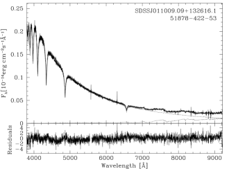
Figure 6: Two-component fit to the spectrum of SDSS 0110+1326. The top panel shows the spectrum of the object as a solid black line and the two templates, white dwarf and M-dwarf, as dotted lines. The bottom panel shows the residuals from the fit.

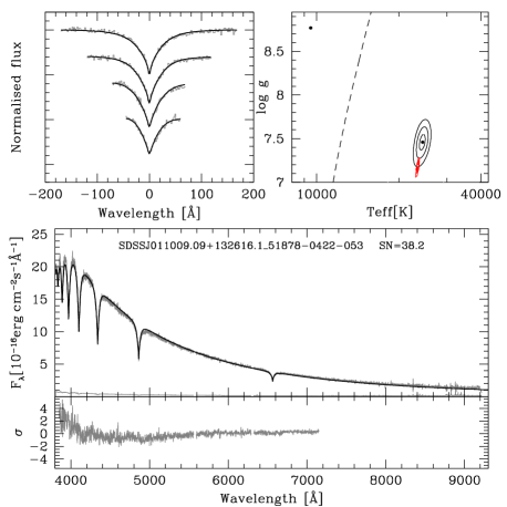
Figure 7: Spectral model fit to the white dwarf in SDSS 0110+1326, obtained after subtracting the best-fit M-dwarf template. Top left panel: best-fit (black lines) to the observed $\mathrm{H}\beta$ to $\mathrm{H}\epsilon$ (gray lines, top to bottom) line profiles. The model spectra and observations have been normalised in the same way. Top right panel: 1, 2 and 3 $\sigma$ contour plots in the $T_{\mathrm{eff}}$-$\log g$ plane. The black contours refer to the best line profile fit, the red ones (which collapse into a dot on the scale of the plot) to the fit of the spectral range 3850–7150 Å. The dashed line indicates the occurrence of maximum $\mathrm{H}\beta$ equivalent width. The best “hot” and “cold” line profile solutions are indicated by black dots, while the best fit to the whole spectrum by a red one. Bottom panel: the residual white dwarf spectrum resulting from the spectral decomposition and their flux errors (gray lines) along with the best-fit white dwarf model (black line) in the 3850–7150 Å wavelength range (top) and the residuals of the fit (gray line, bottom).

We used the spectral decomposition/fitting method described in detail in Rebassa-Mansergas et al. (2007) to estimate the white dwarf effective temperatures ($T_{\mathrm{eff}}$) and surface gravities ($\log g$), as well as the spectral types of the companion stars, for our four targets from their SDSS spectroscopy.

Briefly, the method employed is the following: as a first step a two-component model is fitted to the WDMS binary spectrum using a grid of observed M-dwarf and white dwarf templates. This step determines the spectral type and flux contribution of the M-dwarf component as shown in Fig. 6. After subtracting the best-fit M-dwarf, the residual white dwarf spectrum is fitted with a grid of white dwarf model spectra from Koester et al. (2005). We fit the normalised H$\beta$ to H$\epsilon$ line profiles, omitting $\mathrm{H}\alpha$ which is most severely contaminated by the continuum and/or H$\alpha$ emission from the companion star. Balmer line profile fits can lead to degeneracy in the determination of $T_{\mathrm{eff}}$  and $\log g$, as their equivalent widths (EWs) go through a maximum at $\mbox{$T_{\mathrm{eff}}$}\simeq 13000\,\mathrm{K}$, which means that fits of similar quality can be achieved for a “hot” and “cold” solution. In order to select the physically correct solution, we also fit the continuum plus Balmer lines over the range 3850–7150 Å. The resulting $T_{\mathrm{eff}}$ and $\mathrm{log}g$ are less accurate than those from line profile fits, but sensitive to the slope of the spectrum, and hence allow in most cases to break the degeneracy between the hot and cold solutions. Figure 7 illustrates this procedure. Once $T_{\mathrm{eff}}$ and $\log g$ are determined, the white dwarf mass and radius can be estimated using an updated version of Bergeron et al.’s (1995) tables. The results, after applying this method to our four systems, are summarised in Table 5. The preferred solution (“hot” or “cold”) is highlighted in bold fond.

In the case of SDSS 0303+0054, which contains a DC white dwarf (Fig. 2), the spectral decomposition results in $\mathrm{Sp}(2)=\mathrm{M}4.5\pm 0.5$ for the secondary star. The subsequent fit to the residual white dwarf spectrum is not physical meaningful, as the white dwarf in SDSS 0303+0054 does not exhibit Balmer lines. The fit to the overall spectrum, which is purely sensitive to the continuum slope, suggests $\mbox{$T_{\mathrm{eff}}$}<8000$ K, which is consistent with the DC classification of the white dwarf.

Table 5: Summary of the results obtained for SDSS 0110+1326, SDSS 1435+3733 and SDSS 1548+4057 from our spectral decomposition technique. The preferred set of parameters for each system is highlighted in bold fond.

Solution	$M_{\mathrm{WD}}$[$\mathrm{M}_{\odot}$]	$\log g$	$T_{\mathrm{eff}}$[$\mathrm{K}$]	$\mathrm{Sp}(2)$
SDSS 0110+1326
Hot	0.47$\pm$0.02	7.65$\pm$0.05	25891$\pm$427	M4$\pm$1
Cold	$1.2\pm 0.03$	$9\pm 0.04$	$9619\pm 23$	$\mathrm{M}4\pm 1$
SDSS 1435+3733
Hot	$0.40\pm 0.05$	$7.58\pm 0.11$	$12536\pm 438$	$\mathrm{M}4.5\pm 0.5$
Cold	0.41$\pm$0.05	7.62$\pm$0.12	12536$\pm$488	M4.5$\pm$0.5
SDSS 1548+4057
Hot	$0.43\pm 0.16$	$7.64\pm 0.31$	$14899\pm 1300$	$\mathrm{M}6\pm 0.5$
Cold	0.62$\pm$0.28	8.02$\pm$0.44	11699$\pm$820	M6$\pm$0.5

7 Basic equations

Here, we introduce the set of equations that we will use to constrain the stellar parameters of our four eclipsing WDMS binaries. In a binary system, where a white dwarf primary and a main-sequence companion, with masses $M_{\mathrm{WD}}$ and $M_{\mathrm{sec}}$ respectively, orbit with a period $P_{\mathrm{orb}}$ around their common centre of mass at a separation $a=a_{\mathrm{WD}}+a_{\mathrm{sec}}$ where $a_{\mathrm{WD}}\,\mbox{$M_{\mathrm{WD}}$}\,=\,a_{\mathrm{sec}}\,\mbox{$M_{\mathrm{sec}}$}$, the orbital velocity $K$ of either star, as observed at an inclination angle $i$, is

$$K_{j}=\frac{2\pi a_{j}}{P_{\mathrm{orb}}}\sin i\qquad j=\mathrm{WD,sec}$$ (5)

assuming circular orbits. Given Kepler’s law

$$a^{3}=\frac{\mathrm{G}\left(\mbox{$M_{\mathrm{WD}}$}+\mbox{$M_{\mathrm{sec}}$}\right)P^{2}_{\mathrm{orb}}}{4\pi^{2}}$$ (6)

and using

$$a=a_{\mathrm{WD}}\frac{\mbox{$M_{\mathrm{WD}}$}+\mbox{$M_{\mathrm{sec}}$}}{\mbox{$M_{\mathrm{sec}}$}}$$ (7)

one can obtain the two mass functions:

$$f\left(\mbox{$M_{\mathrm{sec}}$}\right)=\frac{\left(\mbox{$M_{\mathrm{sec}}$}\sin i\right)^{3}}{\left(\mbox{$M_{\mathrm{WD}}$}+\mbox{$M_{\mathrm{sec}}$}\right)^{2}}=\frac{P_{\mathrm{orb}}K^{3}_{\mathrm{WD}}}{2\pi G}\quad<\mbox{$M_{\mathrm{sec}}$}$$ (8)

$$f\left(\mbox{$M_{\mathrm{WD}}$}\right)=\frac{\left(\mbox{$M_{\mathrm{WD}}$}\sin i\right)^{3}}{\left(\mbox{$M_{\mathrm{WD}}$}+\mbox{$M_{\mathrm{sec}}$}\right)^{2}}=\frac{P_{\mathrm{orb}}K^{3}_{\mathrm{sec}}}{2\pi G}\quad<\mbox{$M_{\mathrm{WD}}$}$$ (9)

which give strict lower limits on the masses of the components. From these two equations we get

$$q=\frac{\mbox{$M_{\mathrm{sec}}$}}{\mbox{$M_{\mathrm{WD}}$}}=\frac{K_{\mathrm{WD}}}{K_{\mathrm{sec}}}$$ (10)

Therefore, the knowledge of the radial velocities of both stars can immediately yield the mass ratio $q$ of the system, using Eq. (10). In our case, since we lack a measurement for the radial velocity of the white dwarf $K_{\mathrm{WD}}$, a more indirect approach needs to be followed. Re-arranging Eq. (9) for $\sin i$ yields

$$\sin i=\left[\frac{P_{\mathrm{orb}}K^{3}_{\mathrm{sec}}}{2\pi G}\frac{\left(\mbox{$M_{\mathrm{WD}}$}+\mbox{$M_{\mathrm{sec}}$}\right)^{2}}{M^{3}_{\mathrm{WD}}}\right]^{1/3}$$ (11)

whereas re-arranging Eq. (9) for $K_{\mathrm{sec}}$ yields

$$K_{\mathrm{sec}}=\left[\frac{2\pi G\sin^{3}i}{P_{\mathrm{orb}}}\frac{M^{3}_{\mathrm{WD}}}{\left(\mbox{$M_{\mathrm{WD}}$}+\mbox{$M_{\mathrm{sec}}$}\right)^{2}}\right]^{1/3}$$ (12)

We make use of Equations (11) and (12) in the light curve fitting process described in the next section.

For the DC white dwarf in SDSS 0303+0054, where we lack a spectroscopic estimate of $M_{\mathrm{WD}}$, we can use Eq. (9) to get a rough, first estimate of the white dwarf mass. In Fig. 8, we have plotted Eq. (9) for $i=90^{\circ}$ and $i=78^{\circ}$. For lower inclinations no eclipses occur for $K_{\mathrm{sec}}=339.7\,\mbox{$\mathrm{km\,s^{-1}}$}$ and $\mbox{$P_{\mathrm{orb}}$}=0.134$ d. For a given choice of the inclination angle, Eq. (9) defines a unique relation $\mbox{$M_{\mathrm{sec}}$}\left(\mbox{$M_{\mathrm{WD}}$}\right)$. If we further assume a mass for the secondary, we can investigate the possible range of the white dwarf mass for SDSS 0303+0054. For an extremely conservative lower limit of $\mbox{$M_{\mathrm{sec}}$}\geq 0.08\,\mbox{$\mathrm{M}_{\odot}$}$ (the lower mass limit for an M-dwarf, e.g. Dorman et al. (1989), with the spectrum of SDSS 0303+0054 clearly identifying the companion as a main-sequence star), $\mbox{$M_{\mathrm{WD}}$}\geq 0.68\,\mbox{$\mathrm{M}_{\odot}$}$. Even under this extreme assumption for the companion star, the white dwarf in SDSS 0303+0054 has to be more massive than the average field white dwarf (Koester et al., 1979; Liebert et al., 2005). If we assume $\mathrm{Sp}(2)=\mathrm{M}4$, the upper limit of the spectral type according to our spectral decomposition of the SDSS spectrum, and use the spectral type-mass relation of Rebassa-Mansergas et al. (2007), we find $\mbox{$M_{\mathrm{sec}}$}\simeq 0.32\,\mbox{$\mathrm{M}_{\odot}$}$, and hence $\mbox{$M_{\mathrm{WD}}$}\geq 0.96\,\mbox{$\mathrm{M}_{\odot}$}$. These estimates assume $i=90^{\circ}$, for lower inclinations the respective $M_{\mathrm{WD}}$ values become larger, as illustrated in Fig. 8. In summary, based on $K_{\mathrm{sec}}$, $P_{\mathrm{orb}}$, and a generous range in possible $M_{\mathrm{sec}}$  we expect the white dwarf in SDSS 0303+0054 to be fairly massive, $0.7\mbox{$\mathrm{M}_{\odot}$}\la\mbox{$M_{\mathrm{WD}}$}\la 1.0\mbox{$\mathrm{M}_{\odot}$}$.

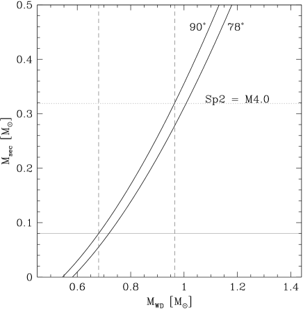
Figure 8: Mass function plot (see Eq. 9) for SDSS 0303+0054, for $i=78^{\circ}$ and $i=90^{\circ}$. The gray horizontal line corresponds to a lower mass limit for M-dwarfs. The dotted horizontal line is the value of $M_{\mathrm{sec}}$, corresponding to a secondary spectral type of $\mathrm{Sp}(2)=\mathrm{M}4$, assuming a $\mathrm{Sp}(2)-\mbox{$M_{\mathrm{sec}}$}$ relation. The dashed vertical lines indicate the corresponding range for the white dwarf mass.

8 Light Curve model fitting

Analysing the light curves of eclipsing binaries can provide strong constraints on the physical parameters of both stars. Here, we make use of a newly developed code written by one of us (TRM) for the general case of binaries containing a white dwarf. The code offers the option to include accretion components (disc, bright spot) for the analysis of cataclysmic variables – given the detached nature of our targets, those components were not included. The program sub-divides each star into small elements with a geometry fixed by its radius as measured along the direction of centres towards the other star. The code allows for the distortion of Roche geometry and for irradiation of the main-sequence star using the approximation $\sigma T_{\mathrm{sec}}^{{}^{\prime}4}=\sigma T_{\mathrm{sec}}^{4}+F_{\mathrm{irr}}$, where $T^{\prime}_{\mathrm{sec}}$ is the modified temperature and $T_{\mathrm{sec}}$ the temperature of the unirradiated companion, $\sigma$ is the Stefan-Boltzmann constant and $F_{\mathrm{irr}}$ is the irradiating flux, accounting for the angle of incidence and distance from the white dwarf. The white dwarf is treated as a point source in this calculation and no backwarming of the white dwarf is included. The latter is invariably negligible, while the former is an unnecessary refinement given the approximation inherent in treating the irradiation in this simple manner.

The code computes a model based on input system parameters supplied by the user. Starting from this parameter set, model light curves are then fitted to the data using Levenberg-Marquardt minimisation, where the user has full flexibility as to which parameters will be optimised by the fit, and which ones will be kept fixed at the initial value.

The physical parameters, which define the models, are the radii scaled by the binary separation, $\mbox{$R_{\mathrm{WD}}$}/a$ and $\mbox{$R_{\mathrm{sec}}$}/a$, the orbital inclination, $i$, the unirradiated stellar temperatures of the white dwarf and the secondary star $T_{\mathrm{eff,WD}}$ and $T_{\mathrm{eff,sec}}$ respectively, the mass ratio $q=\mbox{$M_{\mathrm{sec}}$}/\mbox{$M_{\mathrm{WD}}$}$, $T_{0}$ the time of mid-eclipse of the white dwarf and $d$ the distance. We account for the distance simply as a scaling factor that can be calculated very rapidly for any given model, and so it does not enter the Levenberg-Marquardt optimisation. All other parameters can be adjusted, i.e. be allowed to vary during the fit, but typically the light-curve of a given system does not contain enough information to constrain all of them simultaneously. For instance, for systems with negligible irradiation, fitting $T_{\mathrm{eff,WD}}$, $T_{\mathrm{eff,sec}}$ and $d$ simultaneously is degenerate since a change in distance can be exactly compensated by changes in the temperatures.

Some of our exposures were of a significant length compared to the length of the white dwarf’s ingress and egress and therefore we sub-divided the exposures during the model calculation, trapezoidally averaging to obtain the estimated flux.

Our aim is to combine the information from the $K_{\mathrm{sec}}$ radial velocity amplitudes determined in Sect. 5, the information contained in the light curve, and the white dwarf effective temperature determined from the spectral fit in Sect. 6 to establish a full set of stellar parameters for the four eclipsing WDMS binaries. The adopted method is described in the next two subsections, where SDSS 0110+1326 requires a slightly broader approach, as a correction needs to be applied to the $K_{\mathrm{sec}}$ velocity determined from the emission lines.

8.1 SDSS 0303+0054, SDSS 1435+3733 and SDSS 1548+4057

Our approach is to fit a light curve model to the data for a selected grid of points in the $\mbox{$M_{\mathrm{WD}}$}-\mbox{$M_{\mathrm{sec}}$}$ plane. Each point in the $\mbox{$M_{\mathrm{WD}}$}-\mbox{$M_{\mathrm{sec}}$}$ plane defines a mass ratio $q$ (Eq. 10), and, using $K_{\mathrm{sec}}$ and $P_{\mathrm{orb}}$, a binary inclination $i$ (Eq. 11). Hence, a light curve fit for a given ($M_{\mathrm{WD}}$, $M_{\mathrm{sec}}$) combination will have $M_{\mathrm{WD}}$, $M_{\mathrm{sec}}$, $q$, and $i$ fixed, whereas $R_{\mathrm{WD}}$, $R_{\mathrm{sec}}$, $T_{\mathrm{eff,sec}}$, $T_{\mathrm{eff,WD}}$, and $T_{0}$ are in principle free parameters. In practice, we fix $T_{\mathrm{eff,WD}}$ to the value determined from the spectroscopic fit, which is sufficiently accurate, hence only $R_{\mathrm{WD}}$, $R_{\mathrm{sec}}$, $T_{\mathrm{eff,sec}}$, and $T_{0}$ are free parameters in the light curve fits. We leave $T_{0}$ free to vary to account for the $O-C$ errors in each individual light curve. The fitted values of $T_{0}$ were of the order of 10 s, consistent with the $O-C$ values quoted in Table 3. Each light curve fit in the $\mbox{$M_{\mathrm{WD}}$}-\mbox{$M_{\mathrm{sec}}$}$ plane requires some initial estimates of $R_{\mathrm{WD}}$, $R_{\mathrm{sec}}$, $T_{\mathrm{eff,sec}}$. For $R_{\mathrm{WD}}$  we adopt the theoretical white dwarf mass-radius relation interpolated from Bergeron et al.’s (1995) tables. For $R_{\mathrm{sec}}$  we use the mass-radius relation of Baraffe et al. (1998), adopting an age of 5 Gyr. For $T_{\mathrm{eff,sec}}$, we use the spectral type of the secondary star as determined from the spectral decomposition (Sect. 6) combined with the spectral type-temperature relation from Rebassa-Mansergas et al. (2007). $R_{\mathrm{WD}}$ and $R_{\mathrm{sec}}$ are then scaled by the binary separation, Eq. (7).

We defined large and densely covered grids of points in the $\mbox{$M_{\mathrm{WD}}$}-\mbox{$M_{\mathrm{sec}}$}$ plane which generously bracket the initial estimates for $M_{\mathrm{WD}}$ and $M_{\mathrm{sec}}$ based on the spectral decomposition/fitting. For SDSS 0303+0054, where no spectral fit to the white dwarf is available, we bracket the range in $M_{\mathrm{WD}}$ illustrated in Fig. 8. Points for which (formally) $\sin i>1$ were discarded from the grid, for all other points a light curve fit was carried out, recording the resulting $R_{\mathrm{WD}}$, $R_{\mathrm{sec}}$, and $T_{\mathrm{eff,sec}}$. The number of light curve fits performed for each system was between 7000 and 10000, depending on the system.

8.2 SDSS 0110+1326

In the case of SDSS 0110+1326 the inclination angle cannot readily be calculated through Eq. (11), as we measured $K_{\mathrm{sec}}$ from either the H$\alpha$ or Ca II emission lines, which do not trace the motion of the secondary’s centre of mass, but the centre of light in the given emission line. The general approach in this case is to apply a correction to the observed $K_{\mathrm{sec}}$, where the motion of the secondary star’s centre of mass, $K_{\mathrm{sec\,,cor}}$ is expressed according to Wade & Horne (1988) as

$$K_{\mathrm{sec,\,cor}}=\frac{K_{\mathrm{sec}}}{1-\left(1+q\right)\left(\Delta R/a\right)}$$ (13)

where $K_{\mathrm{sec}}$ is the measured radial velocity, $q$ is the mass ratio of the system, $a$ the binary separation and $\Delta$R is the displacement of the centre of light from the centre of mass of the secondary. $\Delta R$ can have a minimum value of zero, i.e. the two centres coincide and no correction is needed and a maximum value of $R_{\mathrm{sec}}$, i.e. all light comes from a small region of the secondary star closest to the primary. An assumption often used in the literature is that the emission due to irradiation is distributed uniformly over the inner hemisphere of the secondary star, and is zero on its unirradiated side, in which case $\Delta R=\left(4/3\pi\right)$$R_{\mathrm{sec}}$ (e.g. Wade & Horne, 1988; Wood et al., 1995b; Orosz et al., 1999; Vennes et al., 1999). A more physical model of the distribution of the irradiation-induced emission line flux can be derived from the analysis of the orbital variation of the equivalent width of the emission line. A fine example of this approach is the detailed study of the Ca II $\lambda\lambda$ 8498.02, 8542.09,8662.14 emission in the WDMS binary HR Cam presented by Maxted et al. (1998). However, given the small number of spectra, it is currently not possible to apply this method to SDSS 0110+1326.

Our approach for modelling SDSS 0110+1326 was to calculate the binary separation from Eq. (6) for each pair of $\left(\mbox{$M_{\mathrm{WD}}$},\mbox{$M_{\mathrm{sec}}$}\right)$ of the initial grid and then, using Eq. (13), calculate various possible $K_{\mathrm{sec,\,cor}}$ values for this $\left(\mbox{$M_{\mathrm{WD}}$},\mbox{$M_{\mathrm{sec}}$}\right)$ point, assuming various forms of $\Delta R$. We adopted the following three different cases: (i) $\Delta R=0$, i.e. the centre of light coincides with the centre of mass, (ii) $\Delta R=\left(4/3\pi\right)$$R_{\mathrm{sec}}$, i.e. the uniform distribution case and (iii) $\Delta R=$$R_{\mathrm{sec}}$, i.e. the maximum possible displacement of the centre of light. This was done for both the $\mathrm{H}\alpha$ and the Ca II lines. Having attributed a set of corrected radial velocity values to each point of the grid, we could now make use of Eq. (11) to calculate the corresponding inclination angles. Again, points with a (formal) $\sin i>1$ were eliminated from the grid. The allowed $\left(\mbox{$M_{\mathrm{WD}}$},\mbox{$M_{\mathrm{sec}}$}\right)$ pairs for both lines and all three $\Delta R$ cases are shown in Fig. 9.

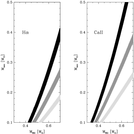
Figure 9: Grid of $(\mbox{$M_{\mathrm{WD}}$},\mbox{$M_{\mathrm{sec}}$})$ points for which the light curve of SDSS 0110+1326 has been fitted. Different assumptions for the $K$-correction were made: $\Delta R=0$ (black strip), $\Delta R=(4/3\pi)\mbox{$R_{\mathrm{sec}}$}$ (dark gray strip) and $\Delta R=\mbox{$R_{\mathrm{sec}}$}$ (light gray strip). Left panel: ($M_{\mathrm{WD}}$,$M_{\mathrm{sec}}$) grid for $K_{\mathrm{sec}}=K_{\mathrm{sec,\,H}\alpha}=200.1\,\mbox{$\mathrm{km\,s^{-1}}$}$. Right panel: ($M_{\mathrm{WD}}$,$M_{\mathrm{sec}}$) grid for $K_{\mathrm{sec}}=K_{\mathrm{sec,\,Ca{\,\scriptsize II}}}=178.8\,\mbox{$\mathrm{km\,s^{-1}}$}$.

The first of the three $\Delta R$ cases, $\Delta R=0$, is obviously not a physically correct approach, as it implies that no correction is necessary. However, we did use it as a strict lower limit of the radial velocity of the secondary. In this sense, the third case, $\Delta R=$$R_{\mathrm{sec}}$, is a strict upper limit for $K_{\mathrm{sec}}$. Table 6 lists the ranges $K_{\mathrm{sec},\mathrm{cor}}$ corresponding the our adopted grid in the $\left(\mbox{$M_{\mathrm{WD}}$},\mbox{$M_{\mathrm{sec}}$}\right)$ plane shown in Fig. 9.

Table 6: Corrected values of the radial velocity of the secondary star in SDSS 0110+1326, after assuming a form of $\Delta R$, for both the cases of the $\mathrm{H}\alpha$ and the Ca II emission lines.

$\Delta R$	mean [$\mathrm{km\,s^{-1}}$]	std.dev.	range [$\mathrm{km\,s^{-1}}$]
$\mathbf{\mathrm{H}\alpha}$
0	200.1	-	-
$\left(4/3\pi\right)R_{\mathrm{sec}}$	213.1	2.7	207.9-218.2
$R_{\mathrm{sec}}$	225.2	3.5	218.5-232.1
Ca II
0	178.8	-	-
$\left(4/3\pi\right)R_{\mathrm{sec}}$	195.1	4.2	186.6-202.7
$R_{\mathrm{sec}}$	209.1	6.1	197.2-219.9

9 Results

Our light curve fitting procedure outlined in Sect. 8 yields fitted values for $R_{\mathrm{WD}}$, $R_{\mathrm{sec}}$, and $T_{\mathrm{eff,sec}}$ for a large grid in the $\mbox{$M_{\mathrm{WD}}$}-\mbox{$M_{\mathrm{sec}}$}$ plane, where each $(\mbox{$M_{\mathrm{WD}}$},\mbox{$M_{\mathrm{sec}}$})$ point defines $q$ and $i$. Analysing these results was done in the following fashion.

In a first step, we applied a cut in the quality of the light curve fits, where we considered three different degrees of “strictness” by culling all models whose $\chi^{2}$ was more than 1, 2 or 3$\sigma$ above the best-fit value. This typically left us with a relatively large degeneracy in $M_{\mathrm{WD}}$ and $M_{\mathrm{sec}}$.

In a second step, we had to select among various equally good light curve fits those that are physically plausible. Given that our set of fitted parameters was underconstrained by the number of observables, we had to seek input from theory in the form of mass-radius relations for the white dwarf (using the tables of Bergeron et al. 1995) and for the M-dwarf (using the $5.0$ Gyr model of Baraffe et al. 1998). We then calculated for each model the relative difference between the theoretical value of the radius and the value of the radius from the fit,

$$\delta R=\left|\frac{R_{\mathrm{fit}}-R_{\mathrm{th}}}{R_{\mathrm{th}}}\right|,$$ (14)

where $R_{\mathrm{fit}}$ and $R_{\mathrm{th}}$ are the radius obtained from the light curve fit, and the radius from the mass-radius relation, respectively. Assuming that the binary components obey, at least to some extent, a theoretical mass-radius relation, we defined cut-off values of $\delta R=5\%$, 10%, and 15%, above which light curve models will be culled. The maximum of $\delta R=15\%$ was motivated by the radius excess over theoretical main-sequence models observed in eclipsing low-mass binaries (Ribas et al., 2007), and by the current observational constraints on the white dwarf mass-radius relation (Provencal et al., 1998). This cut in radius was applied individually for the white dwarf, ($\delta R_{\mathrm{WD}}$) and the companion star ($\delta R_{\mathrm{sec}}$).

Combining both the $\chi^{2}$ and $\delta R$ cuts left us in general with a relatively narrow range of system parameters that simultaneously satisfy the radial velocity amplitude and the morphology of the light curve. In a final step, we examined how well the stellar masses determined from the light curve/radial velocity analysis agreed with those derived from the spectral decomposition.

9.1 SDSS 0303+0054

Modelling the light curve of SDSS 0303+0054 involved the following two problems. Firstly, the time resolution of our data set poorly resolves the white dwarf ingress and egress phases, and consequently the white dwarf radius can only be loosely constrained. We decided therefore to fix the white dwarf radius in the light curve fits to the value calculated from the adopted white dwarf mass-radius relation of Bergeron et al. 1995. Secondly, the light curve displays a strong, but slightly asymmetric ellipsoidal modulation, with the two maxima being of unequal brightness (Fig. 1). Similar light curve morphologies have been observed in the WDMS binaries BPM 71214 (Kawka & Vennes, 2003) and LTT 560 (Tappert et al., 2007), and have been attributed to star spots on the secondary star. By design, our light curve model can not provide a fit that reproduces the observed asymmetry. Having said this, the presence of ellipsoidal modulation provides an additional constraint on $R_{\mathrm{sec}}$ that is exploited by the light curve fit.

A number of models passed the strictest configuration of our cut-offs, i.e. $1\sigma$ and $\delta\mbox{$R_{\mathrm{sec}}$}=5\%$ (no cut was used in $\delta\mbox{$R_{\mathrm{WD}}$}$, as $R_{\mathrm{WD}}$ has been fixed during the fits). The possible range of solutions in the $\mbox{$M_{\mathrm{WD}}$}-\mbox{$M_{\mathrm{sec}}$}$ plane is shown in Fig. 10.

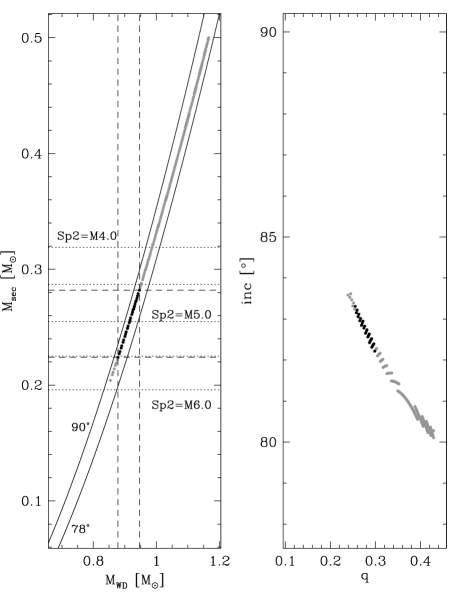
Figure 10: Light curve model fitting results for SDSS 0303+0054. Left panel: $M_{\mathrm{WD}}$  and $M_{\mathrm{sec}}$  values corresponding to fits with $\chi^{2}$ values within $1\sigma$ of the minimum value (gray points) and, simultaneously, with $\delta\mbox{$R_{\mathrm{sec}}$}\leq 0.05$ (black points). Right panel: the same, only in the $q-i$ plane. Also depicted in the left panel are curves corresponding to the mass function (solid black lines, $i=90^{\circ}$ and $78^{\circ}$) which (by definition) bracket the possible solutions, $\mathrm{Sp}(2)-\mbox{$M_{\mathrm{sec}}$}$ relations (dotted, horizontal, black lines) and the range of possible $\left(\mbox{$M_{\mathrm{WD}}$},\mbox{$M_{\mathrm{sec}}$}\right)$ values (dashed, horizontal and vertical, black lines)

Gray dots designate those light curve fits making the 1$\sigma$ cut, black dots those that satisfy both the 1$\sigma$ and $\delta\mbox{$R_{\mathrm{sec}}$}=5\%$ cuts. The resulting ranges in white dwarf masses and secondary star masses are $\mbox{$M_{\mathrm{WD,lcfit}}$}=0.88-0.95\,\mbox{$\mathrm{M}_{\odot}$}$ and $\mbox{$M_{\mathrm{sec}}$}=0.22-0.28\,\mbox{$\mathrm{M}_{\odot}$}$, respectively, corresponding to a white dwarf radius of $\mbox{$R_{\mathrm{WD}}$}=0.008-0.009\,\mbox{$\mathrm{R}_{\odot}$}$ and a secondary radius of $\mbox{$R_{\mathrm{sec}}$}=0.25-0.27\,\mbox{$\mathrm{R}_{\odot}$}$. Fig. 11 shows one example of the light curve fits within this range for the model parameters $\mbox{$M_{\mathrm{WD}}$}=0.91\,\mbox{$\mathrm{M}_{\odot}$}$, $\mbox{$R_{\mathrm{WD}}$}=0.009\,\mbox{$\mathrm{R}_{\odot}$}$, $\mbox{$M_{\mathrm{sec}}$}=0.25\,\mbox{$\mathrm{M}_{\odot}$}$, $\mbox{$R_{\mathrm{sec}}$}=0.26\,\mbox{$\mathrm{R}_{\odot}$}$ and $i=82.6^{\circ}$.

To check the consistency of our light curve fits with the results from the spectral decomposition, we indicate in Fig. 10 the radii of M-dwarfs with spectral types $\mathrm{Sp}(2)=\mathrm{M}4-\mathrm{M}6$ in steps of 0.5, based on the spectral type-mass relation given by Rebassa-Mansergas et al. (2007). The secondary star mass from the light curve fit, $\mbox{$M_{\mathrm{sec,lcfit}}$}=0.23-0.28\,\mbox{$\mathrm{M}_{\odot}$}$, corresponds to a secondary spectral type of $\mathrm{Sp}(2)_{\mathrm{lcfit}}=\mathrm{M}4.5-\mathrm{M}5.5$. The expected spectral type of the secondary from the spectral decomposition (Sect. 6) was $\mathrm{Sp}_{\mathrm{spfit}}(2)=\mathrm{M}4.5\pm 0.5$, hence, both methods yield consistent results.

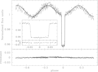
Figure 11: Model fit to the CA2.2 filterless light curve of SDSS 0303+0054, for $\mbox{$M_{\mathrm{WD}}$}=0.91\,\mbox{$\mathrm{M}_{\odot}$}$, $\mbox{$R_{\mathrm{WD}}$}=0.009\,\mbox{$\mathrm{R}_{\odot}$}$, $\mbox{$M_{\mathrm{sec}}$}=0.25\,\mbox{$\mathrm{M}_{\odot}$}$, $\mbox{$R_{\mathrm{sec}}$}=0.26\,\mbox{$\mathrm{R}_{\odot}$}$ and $i=82.6^{\circ}$. The model meets both our $\chi^{2}$ (within $1\sigma$) and the $\delta R$ (within $5\%$) cut-offs. The residuals from the fit are shown at the bottom of the panel. Inset panel: data points and model fit focused around the eclipse.

9.2 SDSS 1435+3733

For SDSS 1435+3733, which is partially eclipsing, our temporal resolution, although again not ideal, was nevertheless deemed to be adequate to constrain the white dwarf radius from the light curve fits. Thus, a $\delta\mbox{$R_{\mathrm{WD}}$}$ cut was also applied.

We applied again our strictest cuts on the light curve models, $1\sigma$ and $\delta\mbox{$R_{\mathrm{WD}}$}=\delta\mbox{$R_{\mathrm{sec}}$}=5\%$, and the parameters of the surviving models are shown in Fig. 12, where the meaning of the symbols is the same as in Fig. 10.

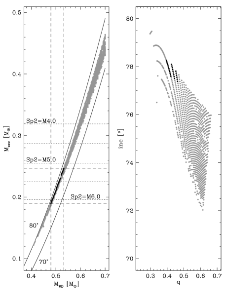
Figure 12: Light curve model fitting results for SDSS 1435+3733. Left panel: $M_{\mathrm{WD}}$  and $M_{\mathrm{sec}}$  values corresponding to fits with $\chi^{2}$ values within $1\sigma$ of the minimum value (gray points) and, simultaneously for both white dwarf and secondary radii, with $\delta R\leq 0.05$ (black points). Right panel: the same, only in the $q-i$ plane. Also depicted in the left panel are mass functions ($i=70^{\circ}$ and $i=80^{\circ}$, solid black lines), $\mathrm{Sp}(2)-\mbox{$M_{\mathrm{sec}}$}$ relations (dotted, horizontal, black lines) and the range of possible $\left(\mbox{$M_{\mathrm{WD}}$},\mbox{$M_{\mathrm{sec}}$}\right)$ values (dashed, horizontal and vertical, black lines)

These fits imply a white dwarf mass and radius of $\mbox{$M_{\mathrm{WD}}$}=0.48-0.53\,\mbox{$\mathrm{M}_{\odot}$}$ and $\mbox{$R_{\mathrm{WD}}$}=0.014-0.015\,\mbox{$\mathrm{R}_{\odot}$}$, respectively, and a secondary star mass and radius of $\mbox{$M_{\mathrm{sec}}$}=0.19-0.25\,\mbox{$\mathrm{M}_{\odot}$}$ and $R_{\mathrm{sec}}$$=0.22-0.25\,\mbox{$\mathrm{R}_{\odot}$}$, respectively. A sample fit that obeyed all three constraints is shown in Fig. 13. The model parameters are $\mbox{$M_{\mathrm{WD}}$}=0.5\,\mbox{$\mathrm{M}_{\odot}$}$, $\mbox{$R_{\mathrm{WD}}$}=0.015\,\mbox{$\mathrm{R}_{\odot}$}$, $\mbox{$M_{\mathrm{sec}}$}=0.21\,\mbox{$\mathrm{M}_{\odot}$}$, $R_{\mathrm{sec}}$$=0.23\,\mbox{$\mathrm{R}_{\odot}$}$ and $i=77.6^{\circ}$.

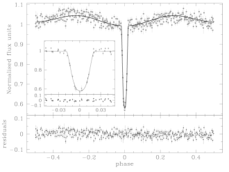
Figure 13: Model fit to IAC80 $I$-band light curve of SDSS 1435+3733, for $\mbox{$M_{\mathrm{WD}}$}=0.5\,\mbox{$\mathrm{M}_{\odot}$}$, $\mbox{$R_{\mathrm{WD}}$}=0.015\,\mbox{$\mathrm{R}_{\odot}$}$, $\mbox{$M_{\mathrm{sec}}$}=0.21\,\mbox{$\mathrm{M}_{\odot}$}$, $\mbox{$R_{\mathrm{sec}}$}=0.23\,\mbox{$\mathrm{R}_{\odot}$}$ and $i=77.6^{\circ}$. The model meets both the $1\sigma$ cut in $\chi^{2}$, and a $\delta R\leq 0.05$ cut for both the white dwarf and the secondary star. The residuals from the fit are shown at the bottom of the panel. Inset panel: data points and model fit focused around the eclipse.

Comparing the white dwarf masses from the spectroscopic decomposition/fit, $\mbox{$M_{\mathrm{WD,spfit}}$}=0.41\pm 0.08\,\mbox{$\mathrm{M}_{\odot}$}$, with the range of white dwarf masses allowed by the light curve fitting, $\mbox{$M_{\mathrm{WD,lcfit}}$}=0.48-0.53\,\mbox{$\mathrm{M}_{\odot}$}$, reveals a reasonable agreement. Regarding the spectral type of the secondary star, we indicate in Fig. 12 again the masses of M-dwarfs in the range M4–M6, in steps of 0.5 spectral classes, following the $\mathrm{Sp}(2)-\mbox{$M_{\mathrm{sec}}$}$ relation of Rebassa-Mansergas et al. (2007). This illustrates that the light curve fits result in a $\mathrm{Sp}(2)_{\mathrm{lcfit}}=\mathrm{M}5-\mathrm{M}6$, whereas the spectral decomposition provided $\mathrm{Sp}(2)_{\mathrm{spfit}}=\mathrm{M}4.5\pm 0.5$. Hence, also the results for the secondary star appear broadly consistent.

Steinfadt et al. (2008) first reported the eclipsing nature of SDSS 1435+3733, and estimated $\mbox{$M_{\mathrm{WD}}$}=0.35-0.58\,\mbox{$\mathrm{M}_{\odot}$}$, $\mbox{$R_{\mathrm{WD}}$}=0.0132-0.0178\,\mbox{$\mathrm{R}_{\odot}$}$, $\mbox{$M_{\mathrm{sec}}$}=0.15-0.35\,\mbox{$\mathrm{M}_{\odot}$}$ and $\mbox{$R_{\mathrm{sec}}$}=0.17-0.32\,\mbox{$\mathrm{R}_{\odot}$}$. The parameter ranges determined from our analysis ($\mbox{$M_{\mathrm{WD}}$}=0.48-0.53\,\mbox{$\mathrm{M}_{\odot}$}$, $\mbox{$R_{\mathrm{WD}}$}=0.014-0.015\,\mbox{$\mathrm{R}_{\odot}$}$, $\mbox{$M_{\mathrm{sec}}$}=0.19-0.25\,\mbox{$\mathrm{M}_{\odot}$}$ and $R_{\mathrm{sec}}$$=0.22-0.25\,\mbox{$\mathrm{R}_{\odot}$}$) are fully consistent with Steinfadt et al.’s work. In Fig. 14 we overplot on the photometry of Steinfadt et al. (2008) the light curve model shown in Fig. 13 along with our data, illustrating that our solution is consistent with their data.

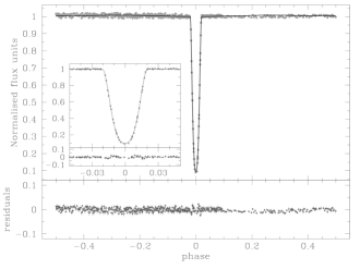
Figure 14: Our light curve model for SDSS 1435+3733, as determined from fitting our IAC80 $I$-band photometry as shown in Fig. 13, along with the data from Steinfadt et al. (2008), illustrating a high degree of consistency.

While the temporal resolution of our photometry is worse than that of Steinfadt et al. (2008), our analysis benefitted from two additional constraints, firstly the mass function (Eq. 9) determined from our spectroscopy, and secondly the detection of a weak ellipsoidal modulation in our $I$-band light curve (Fig. 13). While the observations of Steinfadt et al. (2008) covered the entire binary orbit, their data were obtained through a BG-39 filter, centred at 4800 Å, where the flux contribution of the companion star is negligible. A well-established difficulty in modelling light curves of partially eclipsing binary stars is the fact that, although the sum of the two radii can be accurately defined, their ratio can only be loosely constrained (e.g. Southworth et al., 2007). $R_{\mathrm{WD}}$ and $R_{\mathrm{sec}}$ are strongly correlated, and fitting both of them leads to degeneracy. Additional information is needed to lift this degeneracy, which is mainly provided by ellipsoidal modulation or reflection effects (e.g. Hilditch et al., 1996a, b).

9.3 SDSS 1548+4057

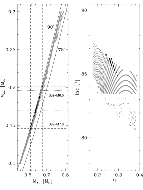
Figure 15: Light curve model fitting results for SDSS 1548+4057. Left panel: $M_{\mathrm{WD}}$  and $M_{\mathrm{sec}}$  values corresponding to fits with $\chi^{2}$ values within $1\sigma$ of the minimum value (gray points) and, simultaneously for both white dwarf and secondary radii, with $\delta R\leq 0.1$ (black points). Right panel: the same, only in the $q-i$ plane. Also depicted in the left panel are mass function for $i=78^{\circ}$ and $i=90^{\circ}$ (solid black lines), $\mathrm{Sp}(2)-\mbox{$M_{\mathrm{sec}}$}$ relations for spectral types M6, 6.5, and 7 (dotted, horizontal, black lines) and the range of possible $(\mbox{$M_{\mathrm{WD}}$},\mbox{$M_{\mathrm{sec}}$})$ values (dashed, horizontal and vertical, black lines).

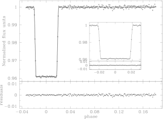
Figure 16: Model fit to the WHT/$R$-band light curve of SDSS 1548+4057, for $\mbox{$M_{\mathrm{WD}}$}=0.65\,\mbox{$\mathrm{M}_{\odot}$}$, $\mbox{$R_{\mathrm{WD}}$}=0.011\,\mbox{$\mathrm{R}_{\odot}$}$, $\mbox{$M_{\mathrm{sec}}$}=0.18\,\mbox{$\mathrm{M}_{\odot}$}$, $\mbox{$R_{\mathrm{sec}}$}=0.183\,\mbox{$\mathrm{R}_{\odot}$}$ and $i=86.6^{\circ}$. The model meets both a $1\sigma$ $\chi^{2}$ cut-off, and the $\delta R\leq 0.10$, cut-off, for both the white dwarf and the secondary radii. The residuals from the fit are shown at the bottom of the panel. Inset panel: data points and model fit focused around the eclipse.

For SDSS 1548+4057, we follow a very similar approach as for SDSS 1435+3733, adopting a $1\sigma$ cut in $\chi^{2}$ but a slightly less strict cut on the radii, $\delta\mbox{$R_{\mathrm{WD}}$}=\delta\mbox{$R_{\mathrm{sec}}$}=10\%$. Figure 15 shows the solutions of our light curve fits that survived those criteria, where plot symbols have the same meaning as in Figs.10 and 12.

The models satisfying both cuts imply a white dwarf mass and radius of $\mbox{$M_{\mathrm{WD}}$}=0.61-0.68\,\mbox{$\mathrm{M}_{\odot}$}$ and $\mbox{$R_{\mathrm{WD}}$}=0.010-0.011\,\mbox{$\mathrm{R}_{\odot}$}$, respectively, and a secondary mass and radius of $\mbox{$M_{\mathrm{sec}}$}=0.15-0.20\,\mbox{$\mathrm{M}_{\odot}$}$ and $\mbox{$R_{\mathrm{sec}}$}=0.17-0.20\,\mbox{$\mathrm{R}_{\odot}$}$, respectively. A sample fit, that obeyed all three constraints, is shown in Fig. 16. The model parameters are $\mbox{$M_{\mathrm{WD}}$}=0.65\,\mbox{$\mathrm{M}_{\odot}$}$, $\mbox{$R_{\mathrm{WD}}$}=0.011\,\mbox{$\mathrm{R}_{\odot}$}$, $\mbox{$M_{\mathrm{sec}}$}=0.18\,\mbox{$\mathrm{M}_{\odot}$}$, $\mbox{$R_{\mathrm{sec}}$}=0.18\,\mbox{$\mathrm{R}_{\odot}$}$ and $i=85.6^{\circ}$.

The white dwarf parameters obtained from the light curve fitting are in full agreement with those derived from the spectral decomposition. The former give a possible range of white dwarf masses of $\mbox{$M_{\mathrm{WD,lcfit}}$}=0.61-0.68\,\mbox{$\mathrm{M}_{\odot}$}$, while the latter yield a value of $\mbox{$M_{\mathrm{WD,spfit}}$}=0.62\pm 0.28\,\mbox{$\mathrm{M}_{\odot}$}$. In Fig. 15, we indicate the masses corresponding to secondary spectral types M6, M6.5, and M7. The spectral fitting points to a $\mathrm{Sp}(2)_{\mathrm{spfit}}=\mathrm{M}6$ secondary. Our models indicate $\mathrm{Sp}(2)_{\mathrm{lcfit}}=\mathrm{M}6-\mathrm{M}7$ again consistent with the spectroscopic result.

9.4 SDSS 0110+1326

Because of the uncertainty in the true $K_{\mathrm{sec}}$ velocity of the secondary star, we inspected a total of six different grids of light curve fits for SDSS 0110+1326 (three K-corrections for each of the observed $K_{\mathrm{sec,\,H\alpha}}$ and $K_{\mathrm{sec,\,Ca{\,\scriptsize II}}}$, see Sect. 8.2 and Table 7), and consequently, this star needs a slightly more extensive discussion compared to the other three systems.

In a first exploratory step, we applied our least strict cut-offs, adopting a $3\sigma$ cut on the fit quality, and a $\delta R=15\%$ cut for both the white dwarf and the secondary star radii. Even with these loose constraints, the $\Delta R=\mbox{$R_{\mathrm{sec}}$}$ case, i.e. assuming that the emission is concentrated on the surface of the secondary closest to the white dwarf, does not produce any solutions that meet the cut-off criteria. For the uniform illumination case, $\Delta R=\left(4/3\pi\right)\mbox{$R_{\mathrm{sec}}$}$, there were no solutions for $K_{\mathrm{sec}}=K_{\mathrm{sec,\,H}\alpha}$, but a few solutions for the $K_{\mathrm{sec}}=K_{\mathrm{sec,\,Ca{\,\scriptsize II}}}$. Finally, a number of solutions existed for the case $\Delta R=0$, i.e. assuming no K-correction, for both H$\alpha$ and Ca II. Table 7 summarises this analysis, and the models that survived the culling defined ranges of ($M_{\mathrm{WD}}$,$M_{\mathrm{sec}}$) pairs which are illustrated in Fig. 17.

Table 7: Summary of the fitting results of SDSS 0110+1326, for all three $\Delta R$ prescriptions, for both the cases of the $\mathrm{H}\alpha$ and the Ca II emission lines. In all cases we applied 3$\sigma$ and $\delta R=15\%$ cut-offs. A ($\surd$) means some models passed the cut-off, whereas a (-) means no models passed.

	$\mathbf{\mathrm{H}\alpha}$	Ca II
$\Delta R=0$	$\surd$	$\surd$
$\Delta R=\left(4/3\pi\right)\mbox{$R_{\mathrm{sec}}$}$	-	$\surd$
$\Delta R=\mbox{$R_{\mathrm{sec}}$}$	-	-

Figure 17: Results of the model fitting of SDSS 0110+1326 for $\mathrm{H}\alpha$ (left panels) and Ca II (right panels), for a $3\sigma$ confidence level and $\delta R<0.15$. Black points correspond to $\Delta R=0$, gray to $\Delta R=\left(4/3\pi\right)$$R_{\mathrm{sec}}$(where applicable, see text for details). Top panels show the $\left(\mbox{$M_{\mathrm{WD}}$},\mbox{$M_{\mathrm{sec}}$}\right)$ plain, bottom panels the $q-i$ plain.

Given that the uniform irradiation prescription, $\Delta R=\left(4/3\pi\right)\mbox{$R_{\mathrm{sec}}$}$ represents a mid-way between the two extreme assumptions $\Delta R=\mbox{$R_{\mathrm{sec}}$}$ and $\Delta R=0$, and that a reasonably large range of possible solutions was found for the Ca II velocities (Fig. 17), we decided to explore tighter $\chi^{2}$ constraints for this case. While a number of light curve models are found within $1\sigma$ of the minimum $\chi^{2}$ value, both $\delta\mbox{$R_{\mathrm{WD}}$}$ and $\delta\mbox{$R_{\mathrm{sec}}$}$ were $\sim 15\%$ in all cases. No models survived if we reduced the value of $\delta R$ in addition to the tighter $\chi^{2}$ constraint.

As an illustration of the quality of the light curve fits achieved, Fig. 18 shows a fit with $\mbox{$M_{\mathrm{WD}}$}=0.59\,\mbox{$\mathrm{M}_{\odot}$}$, $\mbox{$R_{\mathrm{WD}}$}=0.015\,\mbox{$\mathrm{R}_{\odot}$}$, $\mbox{$M_{\mathrm{sec}}$}=0.28\,\mbox{$\mathrm{M}_{\odot}$}$, $\mbox{$R_{\mathrm{sec}}$}=0.32\,\mbox{$\mathrm{R}_{\odot}$}$, $i=85^{\circ}$ and $K_{\mathrm{sec}}=197\,\mbox{$\mathrm{km\,s^{-1}}$}$. The mass of the secondary corresponds to a spectral type of $\mathrm{Sp}(2)=\mathrm{M}4.5$. We stress, however, that we do not adopt this model as a final solution for the parameters of SDSS 0110+1326, but rather consider it as a physically plausible set of parameters.

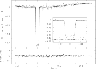
Figure 18: Model fit to the CA2.2 $I$-band light curve of SDSS 0110+1326, for $\mbox{$M_{\mathrm{WD}}$}=0.59\,\mbox{$\mathrm{M}_{\odot}$}$, $\mbox{$R_{\mathrm{WD}}$}=0.015\,\mbox{$\mathrm{R}_{\odot}$}$, $\mbox{$M_{\mathrm{sec}}$}=0.28\,\mbox{$\mathrm{M}_{\odot}$}$, $\mbox{$R_{\mathrm{sec}}$}=0.32\,\mbox{$\mathrm{R}_{\odot}$}$ $i=85^{\circ}$, and $K_{\mathrm{sec}}=197\,\mbox{$\mathrm{km\,s^{-1}}$}$. The model radii agree with the theoretically predicted ones within $15\%$, for both the white dwarf and the secondary star. The residuals from the fit are shown at the bottom of the panel. Inset panel: data points and model fit focused around the eclipse.

Taking the $1\sigma$ confidence levels of the light curve fits at face value, they imply a white dwarf mass of $\mbox{$M_{\mathrm{WD,lcfit}}$}=0.59-0.7\,\mbox{$\mathrm{M}_{\odot}$}$ and a secondary mass of $\mbox{$M_{\mathrm{sec,lcfit}}$}=0.28-0.38\,\mbox{$\mathrm{M}_{\odot}$}$.

For the white dwarf, these numbers are in contrast with the results from the spectral decomposition, $\mbox{$M_{\mathrm{WD,spfit}}$}=0.47\pm 0.02\,\mbox{$\mathrm{M}_{\odot}$}$. The errors in the spectroscopic white dwarf parameters are purely of statistical nature. However, even assuming a reasonably large systematic error of 0.2 dex in $\log g$ (implying $\mbox{$M_{\mathrm{WD,spfit}}$}=0.39-0.55\,\mbox{$\mathrm{M}_{\odot}$}$) the white dwarf masses implied by the light curve fit and the spectroscopic fit appear to be inconsistent.

Regarding the secondary, adopting $\mbox{$M_{\mathrm{sec,lcfit}}$}=0.28-0.38\,\mbox{$\mathrm{M}_{\odot}$}$ and the $\mathrm{Sp}(2)-\mbox{$M_{\mathrm{sec}}$}$ relation of Rebassa-Mansergas et al. 2007 suggests a spectral type of $\mathrm{Sp}(2)_{\mathrm{lcfit}}=\mathrm{M}3-\mathrm{M}4.5$, which is consistent with the results of the spectral decomposition, $\mathrm{Sp}(2)_{\mathrm{spfit}}=\mathrm{M}4\pm 1$.

While our analysis of the light curve fits demonstrates that the data can be modelled well, it is clear that the lack of a reliable value for $K_{\mathrm{sec}}$ prevents the choice of the physically most meaningful solution. Consequently, a definite determination of the stellar parameters of SDSS 0110+1326 is not possible on the basis of the currently available data, and we adopt as a first cautious estimate the values of our spectral decomposition fit. As mentioned in Sect. 8.2, a physically motivated $K$-correction can be modelled once a larger set of spectra covering the entire binary orbit are available.

10 Post common envelope evolution

Considering their short orbital periods, the four new eclipsing WDMS binaries discussed in this paper must have formed through common envelope evolution (Paczynski, 1976; Webbink, 2007). Post common envelope binaries (PCEBs) consisting of a white dwarf and a main sequence star evolve towards shorter orbital periods by angular momentum loss through gravitational radiation and magnetic braking until they enter the semi-detached cataclysmic variable configuration. As shown by Schreiber & Gänsicke (2003), if the binary and stellar parameters are known, it is possible to reconstruct the past and predict the future evolution of PCEBs for a given angular momentum loss prescription. Here, we assume classical disrupted magnetic braking (Rappaport et al., 1983), i.e. magnetic braking is supposed to be much more efficient than gravitational radiation but only present as long as the secondary star has a radiative core. For fully convective stars gravitational radiation is assumed to be the only angular momentum loss mechanism, which applies to all four systems. The current ages of the PCEBs are determined by interpolating the cooling tracks from Wood et al. (1995a). Table 8 lists the evolutionary parameters our four eclipsing WDMS binaries.

Table 8: Reconstructed and predicted orbital periods as well as expected evolutionary times for the four new eclipsing WDMS binaries. The cooling age of the white dwarfs is $t_{\mathrm{cool}}$ while $P_{\mathrm{CE}}$ and $P_{\mathrm{sd}}$ are the orbital periods at the end of the common envelope phase and at the onset of mass transfer, respectively. The time still needed to enter the semi-detached CV configuration is $t_{\mathrm{sd}}$.

SDSS J	$t_{\mathrm{cool}}$ [yr]	$P_{\mathrm{sd}}$ [d]	$P_{\mathrm{CE}}$ [d]	$t_{\mathrm{sd}}$ [yr]
0110+1326	1.41e+07	0.097	0.332	1.78e+10
1548+4057	3.91e+08	0.069	0.191	4.23e+09
0303+0050	3.23e+09	0.097	0.228	5.95e+08
1435+3733	2.53e+08	0.088	0.132	9.50e+08

The calculated evolutionary tracks of the four systems are shown in Fig. 19. The present position of each binary is indicated by an asterisk. The grey-shaded region indicates the $2-3$ h orbital period gap, i.e. the orbital period range where only a small number of cataclysmic variables (CVs) has been found. Given that the four WDMS binaries contain low-mass secondary stars, all of them are expected to start mass transfer in or below the period gap. This underlines the fact first noticed by Schreiber & Gänsicke (2003) that only very few progenitors of long-period CVs are known. SDSS 0303+0050 has passed most of its PCEB lifetime and its current orbital period differs significantly from the reconstructed value at the end of the CE phase. The other three systems are rather young PCEBs with a current orbital period close to $P_{\mathrm{CE}}$.

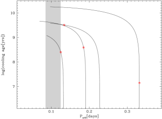
Figure 19: Evolutionary post common envelope tracks for our four eclipsing binaries. From left to right: SDSS 1435+3733, SDSS 1548+4057, SDSS 0303+0054 and SDSS 0110+1326. The current position of the systems is indicated by an asterisk. We assumed only gravitational wave radiation as angular momentum loss agent as all four systems are thought to contain fully convective secondary stars. The orbital period gap of CVs is highlighted in gray – all four systems will start mass transfer in, or shortly below the gap.

11 Conclusions

Table 9: Physical parameters of the known eclipsing white dwarf main sequence binaries. A dash sign means that no corresponding value was given by the respective authors. Errors on the parameters are also shown, if quoted by the authors.

System	$P_{\mathrm{orb}}$ [d]	$M_{\mathrm{WD}}$[$\mathrm{M}_{\odot}$]	$R_{\mathrm{WD}}$[$\mathrm{R}_{\odot}$]	$T_{\mathrm{eff,WD}}$[K]	log$g$	$M_{\mathrm{sec}}$[$\mathrm{M}_{\odot}$]	$R_{\mathrm{sec}}$[$\mathrm{R}_{\odot}$]	$K_{\mathrm{WD}}$ [$\mathrm{km\,s^{-1}}$]	$K_{\mathrm{sec}}$ [$\mathrm{km\,s^{-1}}$]	Sp2	Ref.
V471 Tau	0.521	0.79	0.01	32000	-	0.8	0.85	-	150.7$\pm 1.2$	K2	1a
	0.521	0.84$\pm 0.05$	0.0107$\pm 0.0007$	34500$\pm 1000$	8.31$\pm 0.06$	0.93$\pm 0.07$	0.96$\pm 0.04$	163.6$\pm 3.5$	148.46$\pm 0.56$	K2	1b
RXJ2130.6+4710	0.521	0.554$\pm 0.017$	0.0137$\pm 0.0014$	18000$\pm 1000$	7.93${}^{+0.07}_{-0.09}$	0.555$\pm 0.023$	0.534$\pm 0.017$	136.5$\pm 3.8$	136.4$\pm 0.8$	M3.5-M4	2
DE CVn	0.364	0.51${}^{+0.06}_{-0.02}$	0.0136${}^{+0.0008}_{-0.0002}$	8000$\pm 1000$	7.5	0.41$\pm 0.06$	0.37${}^{+0.06}_{-0.007}$	-	166$\pm 4$	M3V	3
GK Vir	0.344	0.7$\pm 0.3$	-	50000	-	-	-	-	-	M0-M6	4a
	0.344	0.51$\pm 0.04$	0.016	48800$\pm 1200$	7.7$\pm 0.11$	0.1	0.15	-	-	M3-M5	4b
SDSS 1212–0123	0.335	0.46-0.48	0.016-0.018	$17700\pm 300$	7.5-7.7	0.26-0.29	0.28-0.31	-	$181\pm 3$	M4$\pm 1$	5
SDSS 0110+1326	0.332	0.47$\pm 0.2$	0.0163-0.0175	25900$\pm 427$	7.65$\pm 0.05$	0.255-0.38	0.262-0.36	-	180-200	M3-M5	6
RR Cae	0.303	0.365	0.0162	7000	-	0.089	0.134	47.9∗	195.8∗	M6	7a
	0.303	0.467	0.0152	7000	-	0.095	0.189	-	190$\pm 9$	M6	7b
	0.303	0.44$\pm 0.022$	0.015$\pm 0.0004$	7540$\pm 175$	7.61-7.78	0.183$\pm 0.013$	0.188-0.23	79.3$\pm 3$	190.2$\pm 3.5$	M4	7c
SDSS 1548+4057	0.185	0.614-0.678	0.0107-0.0116	11700$\pm 820$	8.02$\pm 0.44$	0.146-0.201	0.166-0.196	-	274.7	M5.5-M6.5	6
EC13471-1258	0.150	0.77$\pm 0.04$	-	14085$\pm 100$	8.25$\pm 0.05$	0.58$\pm 0.05$	0.42$\pm 0.08$	-	241$\pm 8.1$	M2-M4	8a
	0.150	0.78$\pm 0.04$	0.011$\pm 0.01$	14220$\pm 300$	8.34$\pm 0.2$	0.43$\pm 0.04$	0.42$\pm 0.02$	138$\pm 10$	266$\pm 5$	M3.5-M4	8b
CSS 080502†	0.149	$0.35\pm 0.04$	$0.02\pm 0.002$	$17505\pm 516$	$7.38\pm 0.12$	0.32	0.33	-	-	M4	9,6
SDSS 0303+0054	0.134	0.878-0.946	0.0085-0.0093	$<\,$8000	8.4-8.6	0.224-0.282	0.246-0.27	-	339.7	M4-M5	6
NN Ser	0.130	0.57$\pm 0.04$	0.017-0.021	55000$\pm 8000$	7-8	0.10-0.14	0.15-0.18	-	310$\pm 10$	M4.7-M6.1	10a,b
	0.130	0.54$\pm 0.05$	0.0189$\pm 0.001$	57000$\pm 3000$	7.6$\pm 0.1$	0.15$\pm 0.008$	0.174$\pm 0.009$	80.4$\pm 4.1$	289.3$\pm 12.9$	M4.5-M5	10c
SDSS 1435+3733	0.125	-	-	-	-	0.15-0.35	0.17-0.32	-	-	M4-M6	11
	0.125	0.48-0.53	0.0144-0.0153	12500$\pm 488$	7.62$\pm 0.12$	0.19-0.246	0.218-0.244	-	260.9	M4-M5	6
CSS080408‡	-	$0.40\pm 0.05$	$0.022\pm 0.003$	$32595\pm 675$	$7.36\pm 0.17$	0.26	0.27	-	-	M5	9,6
References: (1a) Young & Nelson 1972; (1b) O’Brien et al. 2001; (2) Maxted et al. 2004; (3) van den Besselaar et al. 2007; (4a) Green et al. 1978; (4b) Fulbright et al. 1993; (5) Nebot Gómez-Morán et al. 2008; (6) this work; (7a) Bruch & Diaz 1998; (7b) Bruch 1999; (7c) Maxted et al. 2007; (8a) Kawka et al. 2002; (8b) O’Donoghue et al. 2003; (9) Drake et al. 2008; (10a) Wood & Marsh 1991; (10b) Catalan et al. 1994; (10c) Haefner et al. 2004; (11) Steinfadt et al. 2008
Notes: ∗ Calculated from $K\sin i$ provided by the authors; † CSS080502:090812+060421 = SDSS J090812.04+060421.2, we determined the white dwarf and secondary star paremeters from decomposing/fitting the SDSS spectrum (see Sect. 6 and Rebassa-Mansergas et al. 2007), these parameters should be taken as guidance as no light curve modelling has been done so far; ‡ CSS080408:142355+240925 = SDSSJ142355.06+240924.3, also found by Rebassa-Mansergas et al. (2008a), white dwarf and secondary star parameters determined as for CSS080502.

Since Nelson & Young (1970) reported the discovery of V471 Tau, as the first eclipsing white dwarf main sequence binary, only 7 additional similar systems have been discovered, the latest being SDSS 1435+3733 found by Steinfadt et al. (2008). Here, we presented follow-up observations of SDSS 1435+3733, which we independently identified as an eclipsing WDMS binary, and of three new discoveries: SDSS 0110+1326, SDSS 0303+0050, and SDSS 1548+4057. A fifth system has just been announced by our team (Nebot Gómez-Morán et al., 2008), and two eclipsing WDMS binaries were identified by Drake et al. (2008) in the Catalina Real-Time Transient Survey. Table 9 lists the basic physical parameters of the fourteen eclipsing white dwarf main sequence binaries currently known.

Inspection of Table 9 shows that the orbital periods of the known eclipsing binaries range from three to 12 hours, with three of the systems presented here settling in at the short-period end.

The white dwarf masses cover a range $\sim 0.44-0.9\,\mbox{$\mathrm{M}_{\odot}$}$, with an average of $<\mbox{$M_{\mathrm{WD}}$}>=0.57\pm 0.16\,\mbox{$\mathrm{M}_{\odot}$}$, which is only slightly lower than the average mass of single white dwarfs (Liebert et al., 2005; Finley et al., 1997; Koester et al., 1979). This finding is somewhat surprising, as all these eclipsing WDMS binaries have undergone a common envelope evolution, which is expected to cut short the evolution of the primary star and thereby to produce a significant number of low-mass He-core white dwarfs. Our estimates for the white dwarf masses in SDSS 0110+1326 and SDSS 1435+3733 suggest that they contain He-core white dwarfs. The white dwarf in SDSS 1548+4057 is consistent with the average mass of single white dwarfs. SDSS 0303+0054 contains a fairly massive white dwarf, potentially the most massive one in an eclipsing WDMS binary.

The secondary star masses are concentrated at very low masses, the majority of the fourteen systems in Table 9 have $\mbox{$M_{\mathrm{sec}}$}<0.6$ $\mathrm{M}_{\odot}$, and $\sim 9$ systems (including the four stars discussed here) have $\mbox{$M_{\mathrm{sec}}$}\la 0.3\,\mbox{$\mathrm{M}_{\odot}$}$. This is a range where very few low-mass stars in eclipsing binaries are known (Ribas, 2006), making the secondary stars in eclipsing WDMS binaries very valuable candidates for filling in the empirical mass-radius relation of low mass stars. This aspect will be discussed in a forthcoming paper.

The distribution of secondary star masses among the eclipsing PCEBs in Table 9 is subject to similar selection effects as the whole sample of known PCEBs. Schreiber & Gänsicke (2003) found a strong bias towards late-type secondary stars in the pre-SDSS PCEB population, which arose as most of those PCEBs were identified in blue-colour surveys. The currently emerging population of SDSS PCEBs (Silvestri et al., 2006; Rebassa-Mansergas et al., 2008a) should be less biased as the $ugriz$ – colour-space allows to identify WDMS binaries with a wide range of secondary spectral types and white dwarf temperatures.

Future work will need to be carried out on two fronts. On one hand, more accurate determination of the masses and radii will have to be made to unlock the potential that WDMS binaries hold for testing/constraining the mass-radius relation of both white dwarfs and low mass stars. The key to this improvement are high-quality light curves that fully resolve the white dwarf ingress/egress, and, if possible, the secondary eclipse of the M-dwarf by the white dwarf. In addition, accurate $K_{\mathrm{WD}}$ velocities are needed, which will be most reliably obtained from ultraviolet intermediate resolution spectroscopy. On the other hand, it is clear that the potential of SDSS in leading to the identification of additional eclipsing WDMS binaries has not been exhausted. Additional systems will be identified by the forthcoming time-domain surveys, and hence growing the class of eclipsing WDMS binaries to several dozen seems entirely feasible.

References

- Andersen (1991) Andersen, J., 1991, ARA&A, 3, 91
- Baraffe et al. (1998) Baraffe, I., Chabrier, G., Allard, F., Hauschildt, P. H., 1998, A&A, 337, 403
- Bayless & Orosz (2006) Bayless, A. J., Orosz, J. A., 2006, ApJ, 651, 1155
- Berger et al. (2006) Berger, D. H., et al., 2006, ApJ, 644, 475
- Bergeron et al. (1995) Bergeron, P., Wesemael, F., Beauchamp, A., 1995, PASP, 107, 1047
- Bertin & Arnouts (1996) Bertin, E., Arnouts, S., 1996, A&AS, 117, 393
- Bruch (1999) Bruch, A., 1999, AJ, 117, 3031
- Bruch & Diaz (1998) Bruch, A., Diaz, M. P., 1998, AJ, 116, 908
- Catalan et al. (1994) Catalan, M. S., Davey, S. C., Sarna, M. J., Connon-Smith, R., Wood, J. H., 1994, MNRAS, 269, 879
- Dorman et al. (1989) Dorman, B., Nelson, L. A., Chau, W. Y., 1989, ApJ, 342, 1003
- Drake et al. (2008) Drake, A. J., et al., 2008, ApJ, submitted
- Finley et al. (1997) Finley, D. S., Koester, D., Basri, G., 1997, ApJ, 488, 375
- Fulbright et al. (1993) Fulbright, M. S., Liebert, J., Bergeron, P., Green, R., 1993, ApJ, 406, 240
- Gänsicke et al. (2004) Gänsicke, B. T., Araujo-Betancor, S., Hagen, H.-J., Harlaftis, E. T., Kitsionas, S., Dreizler, S., Engels, D., 2004, A&A, 418, 265
- Green et al. (1978) Green, R. F., Richstone, D. O., Schmidt, M., 1978, ApJ, 224, 892
- Haefner et al. (2004) Haefner, R., Fiedler, A., Butler, K., Barwig, H., 2004, A&A, 428, 181
- Hilditch et al. (1996a) Hilditch, R. W., Harries, T. J., Bell, S. A., 1996a, A&A, 314, 165
- Hilditch et al. (1996b) Hilditch, R. W., Harries, T. J., Hill, G., 1996b, MNRAS, 279, 1380
- Horne (1986) Horne, K., 1986, PASP, 98, 609
- Kawka & Vennes (2003) Kawka, A., Vennes, S., 2003, AJ, 125, 1444
- Kawka et al. (2002) Kawka, A., Vennes, S., Koch, R., Williams, A., 2002, AJ, 124, 2853
- Kawka et al. (2007) Kawka, A., Vennes, S., Dupuis, J., Chayer, P., Lanz, T., 2007, ApJ, in press, arXiv:0711.1526
- Koester et al. (1979) Koester, D., Schulz, H., Weidemann, V., 1979, A&A, 76, 262
- Koester et al. (2005) Koester, D., Napiwotzki, R., Voss, B., Homeier, D., Reimers, D., 2005, A&A, 439, 317
- Liebert et al. (2005) Liebert, J., Bergeron, P., Holberg, J. B., 2005, ApJS, 156, 47
- López-Morales (2007) López-Morales, M., 2007, ApJ, 660, 732
- Marsh (1989) Marsh, T. R., 1989, PASP, 101, 1032
- Maxted et al. (1998) Maxted, P. F. L., Marsh, T. R., Moran, C., Dhillon, V. S., Hilditch, R. W., 1998, MNRAS, 300, 1225
- Maxted et al. (2004) Maxted, P. F. L., Marsh, T. R., Morales-Rueda, L., Barstow, M. A., Dobbie, P. D., Schreiber, M. R., Dhillon, V. S., Brinkworth, C. S., 2004, MNRAS, 355, 1143
- Maxted et al. (2007) Maxted, P. F. L., O’Donoghue, D., Morales-Rueda, L., Napiwotzki, R., 2007, MNRAS, 376, 919
- Morales et al. (2008) Morales, J. C., Ribas, I., Jordi, C., 2008, A&A, 478, 507
- Nebot Gómez-Morán et al. (2008) Nebot Gómez-Morán, A., et al., 2008, A&A, submitted
- Nelson & Young (1970) Nelson, B., Young, A., 1970, PASP, 82, 699
- O’Brien et al. (2001) O’Brien, M. S., Bond, H. E., Sion, E. M., 2001, ApJ, 563, 971
- O’Donoghue et al. (2003) O’Donoghue, D., Koen, C., Kilkenny, D., Stobie, R. S., Koester, D., Bessell, M. S., Hambly, N., MacGillivray, H., 2003, MNRAS, 345, 506
- Orosz et al. (1999) Orosz, J. A., Wade, R. A., Harlow, J. J. B., Thorstensen, J. R., Taylor, C. J., Eracleous, M., 1999, AJ, 117, 1598
- Paczynski (1976) Paczynski, B., 1976, in Eggleton, P., Mitton, S., Whelan, J., eds., IAU Symp. 73: Structure and Evolution of Close Binary Systems, D. Reidel, Dordrecht, p. 75
- Panei et al. (2000) Panei, J. A., Althaus, L. G., Benvenuto, O. G., 2000, A&A, 353, 970
- Provencal et al. (1998) Provencal, J. L., Shipman, H. L., Hog, E., Thejll, P., 1998, ApJ, 494, 759
- Rappaport et al. (1983) Rappaport, S., Joss, P. C., Verbunt, F., 1983, ApJ, 275, 713
- Rebassa-Mansergas et al. (2007) Rebassa-Mansergas, A., Gänsicke, B. T., Rodríguez-Gil, P., Schreiber, M. R., Koester, D., 2007, MNRAS, 382, 1377
- Rebassa-Mansergas et al. (2008a) Rebassa-Mansergas, A., Gänsicke, B., Koester, D., Rodríguez-Gil, P., 2008a, MNRAS, in preparation
- Rebassa-Mansergas et al. (2008b) Rebassa-Mansergas, A., et al., 2008b, MNRAS, 1112
- Ribas (2006) Ribas, I., 2006, Ap&SS, 304, 89
- Ribas et al. (2007) Ribas, I., Morales, J., Jordi, C., Baraffe, I., Chabrier, G., Gallardo, J., 2007, MemSAI, in press, arXiv:0711.4451
- Schreiber & Gänsicke (2003) Schreiber, M. R., Gänsicke, B. T., 2003, A&A, 406, 305
- Schreiber et al. (2008) Schreiber, M. R., Gänsicke, B. T., Southworth, J., Schwope, A. D., Koester, D., 2008, A&A, 484, 441
- Silvestri et al. (2006) Silvestri, N. M., et al., 2006, AJ, 131, 1674
- Southworth & Clausen (2007) Southworth, J., Clausen, J. V., 2007, A&A, 461, 1077
- Southworth et al. (2006) Southworth, J., Gänsicke, B. T., Marsh, T. R., de Martino, D., Hakala, P., Littlefair, S., Rodríguez-Gil, P., Szkody, P., 2006, MNRAS, 373, 687
- Southworth et al. (2007) Southworth, J., Bruntt, H., Buzasi, D. L., 2007, A&A, 467, 1215
- Southworth et al. (2008) Southworth, J., et al., 2008, MNRAS, in press, (arXiv:0809.1753)
- Steinfadt et al. (2008) Steinfadt, J. D. R., Bildsten, L., Howell, S. B., 2008, ApJ Lett., 677, L113
- Tappert et al. (2007) Tappert, C., Gänsicke, B. T., Schmidtobreick, L., Aungwerojwit, A., Mennickent, R. E., Koester, D., 2007, A&A, 474, 205
- Torres (2007) Torres, G., 2007, ApJ Lett., 671, L65
- van den Besselaar et al. (2007) van den Besselaar, E. J. M., et al., 2007, A&A, 466, 1031
- Vennes et al. (1999) Vennes, S., Thorstensen, J. R., Polomski, E. F., 1999, ApJ, 523, 386
- Wade & Horne (1988) Wade, R. A., Horne, K., 1988, ApJ, 324, 411
- Webbink (2007) Webbink, R. F., 2007, in Milone, E., Leahy, D., Hobill, D., eds., Short Period Binary Stars, vol. 352, Springer, p. 233
- Wood & Marsh (1991) Wood, J. H., Marsh, T. R., 1991, ApJ, 381, 551
- Wood et al. (1995a) Wood, J. H., Naylor, T., Marsh, T. R., 1995a, MNRAS, 274, 31
- Wood et al. (1995b) Wood, J. H., Robinson, E. L., Zhang, E.-H., 1995b, MNRAS, 277, 87
- Wood (1995) Wood, M. A., 1995, in Koester, D., Werner, K., eds., White Dwarfs, no. 443 in LNP, Springer, Heidelberg, p. 41
- Young & Nelson (1972) Young, A., Nelson, B., 1972, ApJ, 173, 653