Two-Qubit State Tomography using a Joint Dispersive Read-Out

Abstract

Quantum state tomography is an important tool in quantum information science for complete characterization of multi-qubit states and their correlations. Here we report a method to perform a joint simultaneous read-out of two superconducting qubits dispersively coupled to the same mode of a microwave transmission line resonator. The non-linear dependence of the resonator transmission on the qubit state dependent cavity frequency allows us to extract the full two-qubit correlations without the need for single shot read-out of individual qubits. We employ standard tomographic techniques to reconstruct the density matrix of two-qubit quantum states.

Quantum state tomography allows for the reconstruction of an a-priori unknown state of a quantum system by measuring a complete set of observables Paris and Rehacek (2004). It is an essential tool in the development of quantum information processing Nielsen and Chuang (2000) and has first been used to reconstruct the Wigner-function Schleich (2001) of a light mode Smithey et al. (1993) by homodyne measurements, as suggested in a seminal paper by Vogel and Risken Vogel and Risken (1989). Subsequently, state tomography has been applied to other systems with a continuous spectrum, for instance, to determine vibrational states of molecules Dunn et al. (1995), ions Leibfried et al. (1996) and atoms Kurtsiefer et al. (1997). Later, techniques have been adapted to systems with a discrete spectrum, for example nuclear spins Chuang et al. (1998), polarization entangled photon pairs White et al. (1999), electronic states of trapped ions Roos et al. (2004), states of hybrid atom-photon systems Volz et al. (2006), and spin-path entangled single neutrons Hasegawa et al. (2007).

Recent advances have enabled the coherent control of individual quantum two-level systems embedded in a solid-state environment. Numerous experiments have been performed with superconducting quantum devices Clarke and Wilhelm (2008), manifesting the rapid progress and the promising future of this approach to quantum information processing. In particular, the strong coupling of superconducting qubits to a coplanar waveguide resonator can be exploited to perform cavity quantum electrodynamics (QED) experiments on a chip Wallraff et al. (2004); Blais et al. (2004); Schoelkopf and Girvin (2008) in an architecture known as circuit QED. The high level of control over the dynamics of this coupled quantum system has been demonstrated, e. g., in Leek et al. (2007); Hofheinz et al. (2008). State tomographic methods have already been used in superconducting circuits to verify the entanglement between two phase qubits Steffen et al. (2006). There, the state is determined for each individual qubit with single-shot read-out such that two-qubit correlations can be evaluated by correlating the single measurement outcomes. In contrast, in this letter we extract two-qubit correlations from the simultaneous averaged measurement of two qubits dispersively coupled to a common resonator. This possibility has also been pointed out in Ref. Majer et. el, 2007.

In the setup shown in Fig. 1, two superconducting qubits are coupled to a transmission line resonator operating in the microwave regime Majer et. el (2007).

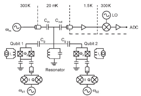
Figure 1: Schematic of the experimental setup with two qubits coupled via the capacitances $\rm{C}_{\rm{g}}$ to a microwave resonator operated at a temperature of about $20~{}\rm{mK}$. The transition frequencies of the qubits are adjusted by external fluxes $\Phi_{1}$ and $\Phi_{2}$. The resonator-qubit system is probed through the input and output capacitances $\rm{C}_{\rm{in}}$ and $\rm{C}_{\rm{out}}$ by a microwave signal at frequency $\omega_{m}$. Additionally, local control of the qubits is implemented by capacitively coupled signals $\omega_{d1}$ and $\omega_{d2}$, which are phase and amplitude modulated using IQ mixers. The output signal is detected in a homodyne measurement at room temperature.

Due to the large dipole moment of the qubits and the large vacuum field of the resonator the strong coupling regime with $g_{1,2}\gg\kappa,\gamma_{1}$ is reached. $g_{1}/2\pi\approx g_{2}/2\pi=133~{}\rm{MHz}$ denotes the similar coupling strenghts of both qubits and $\kappa/2\pi\approx 1.65~{}\rm{MHz}$, $\gamma_{1}/2\pi\approx 0.25~{}\rm{MHz}$ the photon and the qubit decay rates, respectively. The qubits are realized as transmons Koch et al. (2007), a variant of a split Cooper pair box Bouchiat et al. (1998) with exponentially suppressed sensitivy to 1/f charge noise Schreier et al. (2008). The transition frequencies $\omega_{aj}$ ($j=1,2$) of the qubits are tuned separately by external flux bias coils. Both qubits can be addressed individually through local gate-lines using amplitude and phase modulated microwaves at frequencies $\omega_{d1}$ and $\omega_{d2}$. Read-out is accomplished by measuring the transmission of microwaves applied to the resonator input at frequency $\omega_{m}$ close to the fundamental resonator mode $\omega_{r}$. At large detunings $\Delta_{j}\equiv\omega_{aj}-\omega_{r}$ of both qubits from the resonator, the dispersive qubit-resonator interaction gives rise to a qubit state dependent shift of the resonator frequency. In this dispersive limit and in a frame rotating at $\omega_{m}$ the relevant Hamiltonian reads Blais et al. (2007)

$$H = \hbar\big{(}\Delta_{rm}+\chi_{1}\hat{\sigma}_{z1}+\chi_{2}\hat{\sigma}_{z2}\big{)}\hat{a}^{\dagger}\hat{a}$$

$$+\frac{\hbar}{2}\sum_{j=1,2}\left(\omega_{aj}+\chi_{j}\right)\hat{\sigma}_{zj}+\hbar\epsilon(t)(\hat{a}^{\dagger}+\hat{a}),$$

where $\Delta_{rm}\equiv\omega_{r}-\omega_{m}$ is the detuning of the measurement drive from the resonator frequency. The coefficients $\chi_{1,2}$ are determined by the detuning $\Delta_{1,2}$, the coupling strength $g_{1,2}$ and the design parameters of the qubit Koch et al. (2007). The last term in Eq. (Two-Qubit State Tomography using a Joint Dispersive Read-Out) models the measurement drive with amplitude $\epsilon(t)$.

The operator $\hat{\chi}\equiv\chi_{1}\hat{\sigma}_{z1}+\chi_{2}\hat{\sigma}_{z2}$, which describes the dispersive shift of the resonator frequency, is linear in both qubit states. It does not contain two-qubit terms like $\hat{\sigma}_{z1}\hat{\sigma}_{z2}$ from which information about the qubit-qubit correlations could be obtained. However, in circuit QED instead of measuring frequency shifts directly, we record quadrature amplitudes of microwave transmission through the resonator which depend nonlinearly on these shifts. The average values of the field quadratures $\langle\hat{I}(t)\rangle=\operatorname{Tr}[\hat{\rho}(t)(\hat{a}^{\dagger}+\hat{a})]$ and $\langle\hat{Q}\rangle={\mathrm{i}}\operatorname{Tr}[\hat{\rho}(t)(\hat{a}^{\dagger}-\hat{a})]$ are determined from the amplified voltage signal at the resonator output in a homodyne measurement. Here, $\hat{\rho}(t)=U_{m}(t)\hat{\rho}(0)U_{m}(t)^{\dagger}$ denotes the time evolved state of both resonator and qubit under measurement. In the dispersive approximation we can safely assume this state to be separable before the measurement, which is taken to start at time $t_{m}$, $\hat{\rho}(t_{m})=|0\rangle\langle 0|\otimes\hat{\rho}_{q}(t_{m})$. Using these expressions, we find $\langle\hat{Q}(t)\rangle={\mathrm{i}}\operatorname{Tr}_{q}[\hat{\rho}_{q}(t_{m})\langle 0|\hat{U}^{\dagger}_{m}(t)(\hat{a}^{\dagger}-\hat{a})\hat{U}_{m}(t)|0\rangle]$ (and similarly for $\langle\hat{I}(t)\rangle$), where $\operatorname{Tr}_{q}$ denotes the partial trace over the qubit. This expression is evaluated using the input-ouput formalism Gardiner (1992) including cavity decay $\kappa$. In the steady-state, this yields $\langle\hat{I}\rangle_{s},\langle Q\rangle_{s}=-\epsilon\operatorname{Tr}_{q}[\rho_{q}(t_{m})\hat{M}_{I,Q}]$ with

$$\hat{M}_{I} = \frac{2(\Delta_{rm}+\hat{\chi})}{(\Delta_{rm}+\hat{\chi})^{2}+(\kappa/2)^{2}},$$ (2)

$$\hat{M}_{Q} = \frac{\kappa}{(\Delta_{rm}+\hat{\chi})^{2}+(\kappa/2)^{2}}.$$ (3)

We note that the measurement operators are nonlinear functions of $\hat{\chi}$. Thus, $\hat{M}_{I,Q}$ comprises in general also two-qubit correlation terms proportional to $\sigma_{z1}\sigma_{z2}$, which allow to reconstruct the full two-qubit state.

In our experiments the phase of the measurement microwave at frequency $\Delta_{rm}=(\chi_{1}+\chi_{2})$ is adjusted such that the $Q$-quadrature of the transmitted signal carries most of the signal when both qubits are in the ground state. The corresponding measurement operator can be expressed as

$$\hat{M}=\frac{1}{4}\left(\beta_{00}\hat{\text{id}}+\beta_{10}\hat{\sigma}_{z1}+\beta_{01}\hat{\sigma}_{z2}+\beta_{11}\hat{\sigma}_{z1}\hat{\sigma}_{z2}\right),$$ (4)

where $\beta_{ij}=\alpha_{\text{\scriptsize-\,-}}+(-1)^{j}\alpha_{\text{\scriptsize-+}}+(-1)^{i}\alpha_{\text{\scriptsize+\,-}}+(-1)^{i+j}\alpha_{\text{\scriptsize++}}$, with the coefficients

$$\alpha_{\text{\scriptsize$\pm\pm$}}=-\epsilon\kappa\{(\kappa/2)^{2}+(\Delta_{rm}\pm\chi_{1}\pm\chi_{2})^{2}\}^{-1/2}$$ (5)

representing the qubit state dependent $Q$-quadrature amplitudes of the resonator field in the steady-state limit and for infinite qubit-lifetime (Fig. 2(a)).

Since we operate in a regime, where the qubit relaxation cannot be neglected, the steady-state expression is of limited practical use. The decay of a qubit to its ground state changes the resonance frequency of the resonator and consequently limits the read-out time to $\sim 1/\gamma_{1}$. A typical averaged time-trace of the resonator response for pulsed measurements is shown in Fig. 2(b), similar to the data presented in Majer et. el (2007). The qubits are prepared initially in the states $|ee\rangle$, $|eg\rangle$, $|ge\rangle$ and $|gg\rangle$, respectively, using the local gate lines. The time dependence of the measurement signal is determined by the rise time of the resonator and the decay time of the qubits. It is in excellent agreement with calculations (solid lines in Fig. 2(b)) of the dynamics of the dispersive Jaynes-Cummings Hamiltonian Blais et al. (2007); Bianchetti et al. (2008).

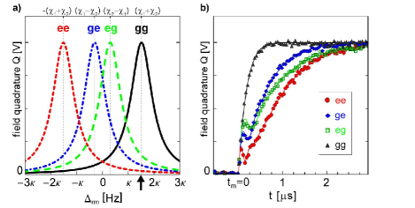
Figure 2: (a) $Q$-quadrature of the resonator field for the qubits in states $gg$, $eg$, $ge$ and $ee$ as a function of the detuning $\Delta_{rm}$. Tomography measurements have been performed at $\Delta_{rm}=(\chi_{1}+\chi_{2})$ indicated by an arrow. (b) Measured (data points) time evolution of the $Q$-quadrature for the indicated initial states compared to numerically calculated responses (solid lines). All parameters have been determined in independent measurements.

Due to the quantum non-demolition nature of the measurement Blais et al. (2004), $\hat{M}$ remains diagonal in the instantaneous qubit eigenbasis during the measurement process. Therefore, a suitable realistic measurement operator $\hat{M}^{\prime}$ can be defined by replacing the $\alpha_{\pm\pm}$ in Eq. (5) with the integrated signal from $t_{m}$ to the final time $T$, $\alpha_{\pm\pm}^{\prime}=1/N\int_{t_{m}}^{T}(\langle\hat{M}(t)\rangle_{\pm\pm}-\langle\hat{M}(t)\rangle_{\text{\scriptsize-\,-}})dt$ with the ground state response $\langle\hat{M}(t)\rangle_{\text{\scriptsize-\,-}}$ subtracted. The normalization constant $N$ is chosen such that $\alpha_{\text{\scriptsize+\,-}}^{\prime}=1$.

To reconstruct the combined state $\hat{\rho}_{q}$ of both qubits, a suitable set of measurements has to be found to determine unambiguously the 16 coefficients $r_{ij}$ of the density matrix $\hat{\rho}_{q}=\sum_{i,j=0}^{3}r_{ij}\,\hat{\sigma}_{i}\otimes\hat{\sigma}_{j}$ with the identity $\hat{\sigma}_{0}=\hat{\text{id}}$ and $\{\hat{\sigma}_{1},\hat{\sigma}_{2},\hat{\sigma}_{3}\}=\{\hat{\sigma}_{x},\hat{\sigma}_{y},\hat{\sigma}_{z}\}$. Such a complete set of measurements is constructed by applying appropriate single qubit rotations $\hat{U}_{k}\in SU(2)\otimes SU(2)$ before the measurement in order to measure the expectation values $\langle\hat{M}_{k}\rangle=\operatorname{Tr}[\hat{M}\hat{U}_{k}\hat{\rho}_{q}\hat{U}_{k}^{\dagger}]=\operatorname{Tr}[\hat{U}_{k}^{\dagger}\hat{M}\hat{U}_{k}\hat{\rho}_{q}]$. The latter equality defines the set of measurement operators $\hat{M}_{k}\equiv\hat{U}_{k}^{\dagger}\hat{M}U_{k}$. This illustrates again that a measurement operator $\hat{M}$ involving non-trivial two-qubit terms $\sigma_{i1}\sigma_{j2}$ is necessary for state tomography. In fact, single-qubit operations $U_{k}=U_{k1}\otimes U_{k2}$ alone cannot be used to generate correlation terms since $U_{k}^{\dagger}(\hat{\text{id}}\otimes\sigma_{z})U_{k}=\hat{\text{id}}\otimes(U_{k2}^{\dagger}\sigma_{z}U_{k2})$, for instance. As $\operatorname{Tr}[(\sigma_{k}\otimes\sigma_{l})(\sigma_{m}\otimes\sigma_{n})]=\delta_{km}\delta_{ln}$, some coefficients $r_{ij}$ of the density matrix $\hat{\rho}_{q}$ would not be determined in an averaged measurement.

To identify the coefficients $r_{ij}$ we perform 16 linearly-independent measurements. The condition for the completeness of the set of tomographic measurements is the non-singularity of the matrix $A$ defined by the relation $\langle\hat{M}_{k}\rangle=\sum_{l=0}^{15}A_{kl}r_{l}$ between the the expectation values $\langle\hat{M}_{k}\rangle$ and the coefficients of the density matrix $r_{l}$ with $l\equiv i+4j$. This condition is only violated if one of the coefficients $\beta_{ij}$ of $\hat{M}$ in Eq. (4) vanishes. For instance, $\beta_{01}=\beta_{10}=0$ for $\Delta_{rm}=0$, which reflects the fact that we cannot distinguish two identical qubits due to symmetry reasons as apparent from Fig. 2(a).

Our pulse scheme for the state tomography is shown in Fig. 3. The transition frequencies of the qubits are adjusted to $\omega_{a1}/2\pi=4.5~{}\rm{GHz}$ and $\omega_{a2}/2\pi=4.85~{}\rm{GHz}$. At this detuning from the resonator frequency $\omega_{r}/2\pi=6.442~{}\rm{GHz}$ the cavity pulls are $\chi_{1}=-1~{}\rm{MHz}$ and $\chi_{2}=-1.5~{}\rm{MHz}$ Koch et al. (2007). First, a given two-qubit state is prepared. Then a complete set of tomography measurements is formed by applying the combination of $\{(\pi/2)_{x},\,(\pi/2)_{y},(\pi),\text{id}\}$ pulses to both qubits over their individual gate lines using amplitude and phase controlled microwave signals. The wanted rotation angles are realized with an accuracy better than $4^{\circ}$. Finally, the measurement drive is applied at $\omega_{m}=6.445~{}\rm{GHz}$ corresponding to the maximum transmission frequency of the resonator with both qubits in the ground state.

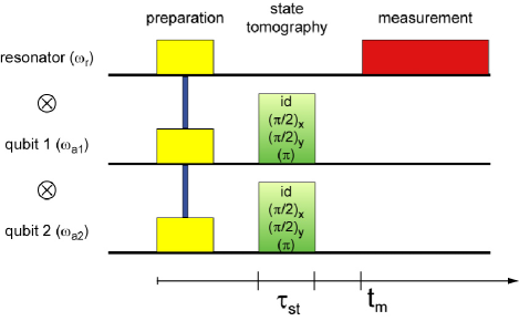
Figure 3: Pulse scheme for state tomography, see text.

To determine the measurement operator $\hat{M}^{\prime}$, $\pi$-pulses are alternately applied to both qubits to yield signals as shown in Fig. 2(b). From this data the coefficients $(\beta_{00}^{\prime},\beta_{01}^{\prime},\beta_{10}^{\prime},\beta_{11}^{\prime})=(0.8,-0.3,-0.4,-0.1)$ of $\hat{M}^{\prime}$ are deduced, where the non-vanishing $\beta_{11}^{\prime}$ allows for a measurement of arbitrary quantum states. As an example of this state reconstruction, in Fig. 4(a) the extracted density matrix $\hat{\rho}_{q}$ of the product state $|\Psi_{\rm{sep}}\rangle=1/\sqrt{2}\left(|g\rangle+|e\rangle\right)\otimes 1/\sqrt{2}\left(|g\rangle+{\mathrm{i}}|e\rangle\right)$ is shown. In Fig. 4(b) the Bell state $|\Phi\rangle=1/\sqrt{2}\left(|g\rangle\otimes|g\rangle-{\mathrm{i}}|e\rangle\otimes|e\rangle\right)$ prepared by a sequence of sideband pulses Wallraff et al. (2007); Blais et al. (2007); Leek et al. (2008) is reconstructed. $6.6\times 10^{4}$ and $6.6\times 10^{5}$ records have been averaged, respectively, for each of the 16 tomographic measurement pulses to determine the expectation values $\langle\hat{M}_{k}^{\prime}\rangle$ for the two states. The corresponding ideal state tomograms are depicted in Fig. 4(c) and (d). To avoid unphysical, non positive-semidefinite, density matrices originating from statistical uncertainties, all tomography data has been processed by a maximum likelihood method Hradil (1997); James et al. (2001). The corresponding fidelities $\mathcal{F}_{\psi}\equiv(\langle\psi|\hat{\rho}_{q}|\psi\rangle)^{1/2}$ are $\mathcal{F}_{\rm{sep}}=95\%$ and $\mathcal{F}_{\Phi^{-}}=74\%$. These results are in close agreement with theoretically expected fidelities when taking finite photon and qubit-lifetimes into account. As a result, the loss in fidelity and concurrence of the Bell state are not due to measurement errors but to the long preparation sequence Leek et al. (2008).

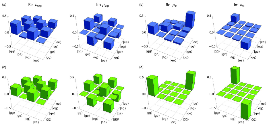
Figure 4: Real and imaginary part of reconstruced density matrices of (a) the product state $|\Psi_{\rm{sep}}\rangle=1/\sqrt{2}\left(|g\rangle+|e\rangle\right)\otimes 1/\sqrt{2}\left(|g\rangle+{\mathrm{i}}|e\rangle\right)$ and (b) the Bell state $|\Phi\rangle=1/\sqrt{2}\left(|g\rangle\otimes|g\rangle-{\mathrm{i}}|e\rangle\otimes|e\rangle\right)$. Ideal tomograms are shown in (c,d).

In conclusion, we have presented a method to jointly and simultaneously read-out the full quantum state of two qubits dispersively coupled to a microwave resonator. In a measurement of the field quadrature amplitudes of microwaves transmitted through the resonator each photon carries information about the state of both qubits. In this way the two-qubit correlations can be extracted from an averaged measurement of the transmission amplitude without the need for single shot or single qubit read-out. This method can also be extended to multi-qubit systems coupled to the same resonator mode.

This work was supported by Swiss National Science Foundation (SNF) and ETH Zurich. P. J. L. was supported by the EC with a MC-EIF, J. M. G. by CIFAR, MITACS and ORDCF and A. B. by NSERC and CIFAR.

References

- Paris and Rehacek (2004) M. Paris and J. Řeháček, eds., Quantum State Estimation (Springer, Berlin, Heidelberg, 2004).
- Nielsen and Chuang (2000) M. A. Nielsen and I. L. Chuang, Quantum Computation and Quantum Information (Cambridge University Press, 2000).
- Schleich (2001) W. Schleich, Quantum Optics in Phase Space (Wiley-VCH, Berlin, 2001).
- Smithey et al. (1993) D. T. Smithey, M. Beck, M. G. Raymer, and A. Faridani, Phys. Rev. Lett. 70, 1244 (1993).
- Vogel and Risken (1989) K. Vogel and H. Risken, Phys. Rev. A 40, 2847 (1989).
- Dunn et al. (1995) T. J. Dunn, I. A. Walmsley, and S. Mukamel, Phys. Rev. Lett. 74, 884 (1995).
- Leibfried et al. (1996) D. Leibfried et al., Phys. Rev. Lett. 77, 4281 (1996).
- Kurtsiefer et al. (1997) C. Kurtsiefer, T. Pfau, and J. Mlynek, Nature 386, 150 (1997).
- Chuang et al. (1998) I. L. Chuang et al., Nature 393, 143 (1998).
- White et al. (1999) A. G. White, D. James, P. Eberhard, and P. Kwiat, Phys. Rev. Lett. 83, 3103 (1999).
- Roos et al. (2004) C. F. Roos et al., Science 304, 1478 (2004).
- Volz et al. (2006) J. Volz et al., Phys. Rev. Lett. 96. 030404 (2006).
- Hasegawa et al. (2007) Y. Hasegawa et al., Phys. Rev. A 76, 052108 (2007).
- Clarke and Wilhelm (2008) J. Clarke and F. K. Wilhelm, Nature 453, 1031 (2008).
- Wallraff et al. (2004) A. Wallraff et al., Nature 431, 162 (2004).
- Blais et al. (2004) A. Blais et al., Phys. Rev. A 69, 062320 (2004).
- Schoelkopf and Girvin (2008) R. Schoelkopf and S. Girvin, Nature 451, 664 (2008).
- Leek et al. (2007) P. J. Leek et al., Science 318, 1889 (2007).
- Hofheinz et al. (2008) M. Hofheinz et al., Nature 454, 310 (2008).
- Steffen et al. (2006) M. Steffen et al., Science 313, 1423 (2006).
- Majer et. el (2007) J. Majer et al., Nature 449, 443 (2007).
- Koch et al. (2007) J. Koch et al., Phys. Rev. A 76,042319 (2007).
- Bouchiat et al. (1998) V. Bouchiat et al., Phys. Scr. T76, 165 (1998).
- Schreier et al. (2008) J. Schreier et al., Phys. Rev. B 77, 180502(R) (2008).
- Blais et al. (2007) A. Blais et al., Phys. Rev. A 75, 032329 (2007).
- Gardiner (1992) C. W. Gardiner, Quantum Noise (Springer, Berlin, 1992).
- Bianchetti et al. (2008) R. Bianchetti et al., in preparation (2008).
- Wallraff et al. (2007) A. Wallraff et al., Phys. Rev. Lett. 99, 050501 (2007).
- Leek et al. (2008) P. J. Leek et al., arXiv:0812.2678 (2008).
- Hradil (1997) Z. Hradil, Phys. Rev. A 55, R1561 (1997).
- James et al. (2001) D. F. V. James, P. G. Kwiat, W. J. Munro, and A. G. White, Phys. Rev. A 64, 052312 (2001).