Solution of the Gribov problem from gauge invariance

Abstract:

A new approach to gauge fixed Yang-Mills theory is derived using the Polyakov-Susskind projection techniques to build gauge invariant states. In our approach, in contrast to the Faddeev-Popov method, the Gribov problem does not prevent the gauge group from being factored out of the partition function. Lattice gauge theory is used to illustrate the method via a calculation of the static quark–antiquark potential generated by the gauge fields in the fundamental modular region of Coulomb gauge.

1 Introduction

Yang-Mills theories are the cornerstone of the standard model. These theories are formulated in terms of a highly redundant set of variables, due to the local gauge symmetry of the action. In case of Yang-Mills theories with matter, the variables are the gauge fields $A_{\mu}(x)$ and the matter fields $Q(x)$. The calculation of physical observables is hampered by the fact that these fields are not directly related to physical particles. This can be easily seen from the fact that they transform non-trivially under gauge transformations $\Omega$ in the gauge group $\cal G$:

$$A_{\mu}(x)\rightarrow A_{\mu}^{\Omega}(x),\hbox to28.45274pt{\hfill}Q(x)\rightarrow\Omega(x)\,Q(x).$$ (1)

Gauge invariance tells us that we can work with any representative of the gauge orbit $\{A_{\mu}^{\Omega}(x)|\Omega(x)\;\in{\cal G}\}$. A common method of choosing a unique representative is through the global maximum of a given gauge fixing action:

$$S_{\mathrm{fix}}[A^{\Omega}]\rightarrow\hbox{global maximum}\hbox to28.45274pt{\hfill}\hbox{for}\hbox to28.45274pt{\hfill}\Omega\;=:\;\Omega_{\mathrm{FMR}}[A].$$ (2)

The set of these representatives is free of Gribov copies and (after suitable boundary identifications) is called the fundamental modular region:

$$\left\{A_{\mu}^{\Omega}(x)\,|\,\Omega=\Omega_{\mathrm{FMR}}[A]\right\}.$$ (3)

It has been known for a long time [1] that a physical electron state $|Q\rangle$ can only be obtained if the bare state $Q(x)|0\rangle$ is properly dressed by a photon cloud:

$$|Q\rangle\,=\,h[A]\,Q(x)|0\rangle\,,\hbox to28.45274pt{\hfill}h[A^{\Omega}]\,=\,h[A]\,\Omega^{\dagger}\;.$$ (4)

The latter equation specifies the dressing property which ensures the gauge invariance of $|Q\rangle$. The choice of a a dressing is not unique. They may differ e.g. by a gauge invariant factor without spoiling the dressing property in (4). One particular way to construct a dressing is to use gauge fixing:

$$h[A]\,=\,\Omega_{\mathrm{FMR}}[A]\;.$$ (5)

We call this definition dressing from the fundamental modular region. Under the assumption that there is a unique global maximum, it can be easily shown that this definition satisfies the dressing property:

$$h[A^{\Omega}]\,=\,\Omega_{\mathrm{FMR}}[A^{\Omega}]=\Omega_{\mathrm{FMR}}[A]\,\Omega^{\dagger}\;=\;h[A]\,\Omega^{\dagger}\;.$$

The disadvantage of this definition is that it relies on an explicit realisation of gauge fixing. While the Faddeev-Popov method [2] works in perturbation theory, it fails non-perturbatively, leading to Green functions being in indeterminate form [3, 4, 5]. This is because in non-Abelian theories the gauge fixing condition has multiple solutions $\Omega(x)$. This was first elucidated by Gribov for the case of Coulomb gauge [6], and since then has been known as the Gribov problem. One might argue that in a purely numerical approach using lattice regularisation there is no need to resort to a gauge fixing condition: one might find the unique representative on the gauge orbit by seeking the global maximum of the gauge fixing action (2) using advanced algorithms. While this approach is conceptually correct, it is not feasible: it can be shown that locating the global maximum is equivalent to solving a spin-glass problem which is beyond the scope of the numerical techniques currently available.

In order to bypass the Gribov problem, we recently proposed [7] combining the alternative construction of the gauge invariant partition function by Parrinello and Zwanziger [8, 9, 10] with the technique of gauge invariant projection initiated by Polyakov and Susskind [11, 12, 13]. This leads to our integral dressing construction of gauge invariant trial states, which we will describe below. We will also describe the “ice-limit”, in which we recover the dressing from the FMR without having to construct the FMR explicitly. As an initial application, we employ the integral dressed trial states to calculate the static interquark potential.

2 Integral dressing

In the following, we will adopt lattice regularisation. The gauge fields $A_{\mu}(x)$ are represented by group valued links $U_{\mu}(x)$. Rather than realising the dressing property (4) by gauge fixing, we define the integral dressing [7]

$$h[U]=\int{\cal D}\Omega\;\;\Omega(x)\;\exp\{\kappa\;S_{\mathrm{fix}}[U^{\Omega}]\},$$ (6)

where $\kappa$ plays the role of a gauge fixing parameter. Using the gauge invariance of the Haar measure, we easily verify the dressing property $(G\in{\cal G})$:

$$h[U^{G}] = \int{\cal D}\Omega\;\;\Omega(x)\;\exp\{\kappa\;S_{\mathrm{fix}}[U^{\Omega G}]\}\;=\;\int{\cal D}[\Omega{G}]\;\;[\Omega{G}]\;{G^{\dagger}}\;\exp\{\kappa\;S_{\mathrm{fix}}[U^{\Omega G}]\}\;=\;h[U]\,{G^{\dagger}}.$$

Gauge invariant dressings for multi-quark trial states may be defined similarly, e.g. for a quark–antiquark trial state we make the ansatz

$$|\mathrm{trial}\rangle:=Q^{\dagger}(y)\;h^{(2)}[U](y,x)\;Q(x)\;|0\rangle,\hbox to28.45274pt{\hfill}h^{(2)}[U]:=\int{\cal D}\Omega\;\;\Omega^{\dagger}(y)\;\Omega(x)\;\exp\{{\kappa}\;S_{\mathrm{fix}}[U^{\Omega}]\}.$$ (7)

Let us briefly discuss the strong gauge fixing limit $\kappa\to\infty$. In this case, the total contribution to the integral in (7) arises solely from the domain where $S_{\mathrm{fix}}$ attains its global maximum. In this case, we recover the dressing from the FMR:

$$h^{(2)}[U]\;\propto\;\Omega_{{}_{\mathrm{FMR}}}^{\dagger}(y)\;\Omega_{{}_{\mathrm{FMR}}}(x),\hbox to28.45274pt{\hfill}|FMR\rangle\,:=\,\lim_{\kappa\to\infty}|\mathrm{trial}\rangle.$$ (8)

As an illustrative example, we consider axial dressing by choosing

$$S_{\mathrm{fix}}[U^{\Omega}]\;=\;\sum_{x}\frac{1}{N_{c}}\,\hbox{tr}\,U^{\Omega}_{3}(x)\;\leq\;N_{x}\;,$$ (9)

where $N_{x}$ is the number of lattice cites, and $N_{c}$ is the number of colours of the gauge group. The key observation is that the upper bound in (9) can be saturated exactly: letting ${\cal C}_{x}$ denote the straight line joining the points $(x_{1},x_{2},1,x_{4})$ and $(x_{1},x_{2},x_{3},x_{4})$, we find $\Omega_{\mathrm{FMR}}(x)\;=\;\prod_{{\cal C}_{x}}U_{3}(x)$ in the strong gauge fixing limit of $\kappa\to\infty$. The integral dressing (8) for a quark at $x$ and an antiquark at $y=x+r\,e_{3}$ then becomes

$$h^{(2)}[U](y,x)\;=\;\prod_{C_{xy}}U_{3}(x),$$ (10)

where $C_{xy}$ is the straight line between $x$ and $y$. Relation (10) and the corresponding trial state have an intuitive interpretation: $h^{(2)}$ is just the Polyakov line between the points $x$ and $y$, so the trial state is made gauge invariant by joining the quark and antiquark with a thin gluonic string.

The static quark antiquark potential $V(r)$ can be obtained by calculating the expectation value of the (Euclidean) time evolution operator using the FMR trial state:

$$\langle\mathrm{trial}|\mathrm{e}^{-HT}|\mathrm{trial}\rangle\stackrel{{\scriptstyle T\,\mathrm{large}}}{{\longrightarrow}}|\langle 2|\mathrm{trial}\rangle|^{2}\;\mathrm{e}^{-V(r)T},\hbox to28.45274pt{\hfill}\langle\mathrm{FMR}|\mathrm{e}^{-HT}|\mathrm{FMR}\rangle=W(r,T).$$ (11)

In the case of the axial dressing, we recover the standard approach to the static potential using rectangular Wilson loops $W(r,t)$. Although we have not encountered here a Gribov problem in the case of axial dressing, its disadvantage is that the overlap $|\langle 2|\mathrm{trial}\rangle|^{2}$ is poor and even vanishes when the lattice regulator is removed [14, 15].

3 Dressing from the Coulomb gauge FMR - the ice-limit

         

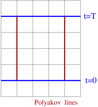
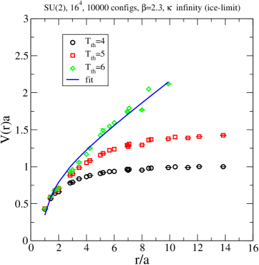
Figure 1: Illustration of the ice-limit (left panel) and the static potential from Coulomb dress trial states (right panel).

A much better overlap is observed if Coulomb gauge fixing is employed [14]:

$$S_{\mathrm{fix}}[U^{\Omega}]\;=\;\sum_{k,x}\frac{1}{N_{c}}\,\hbox{tr}\,U^{\Omega}_{k}(x)\;,\hbox to28.45274pt{\hfill}k=1\ldots 3.$$ (12)

Using the definition of the integral dressing and heavy quark propagation, the expectation value (11) can be written as [7]:

$$\langle\mathrm{trial}|\mathrm{e}^{-HT}|\mathrm{trial}\rangle\propto\int{\cal D}U_{\mu}\;{\cal D}\Omega\;\ldots\;\exp\{{\kappa S_{\mathrm{fix}}[U^{\Omega}]}\}\;.$$ (13)

Note the order of the integration: the $\Omega$ integration is done before the link $U_{\mu}$ integration. With this ordering, we recover the Gribov problem in the large-$\kappa$ limit, since for a given background field $U_{\mu}(x)$, the $\Omega$-path integral may be viewed as a spin-glass partition function with a metric $U_{\mu}(x)$. However, using the explicit gauge invariance of our approach, the order of integration can be exchanged, and the $U$ integral becomes independent of $\Omega$ (for details see  [7]),

$$\langle\mathrm{trial}|\mathrm{e}^{-HT}|\mathrm{trial}\rangle\propto\left(\int{\cal D}\Omega\right)\;\int{\cal D}U_{\mu}\;\ldots\;\exp\{\kappa S_{\mathrm{fix}}[U]\}.$$ (14)

Changing the order of integration solves the Gribov problem: the limit $\kappa\to\infty$ can thus be taken analytically, as the dominant contributions to the integral now arise from maximising (12) with respect to $U$ rather than $\Omega$. The solution is clearly to take $U=1$, i.e.

$$S_{\mathrm{fix}}[U]\stackrel{{\scriptstyle U_{\mu}}}{{\rightarrow}}\hbox{max}\hbox to28.45274pt{\hfill}\implies\hbox to28.45274pt{\hfill}U_{k}(\vec{x},t)=1\;\;\hbox{for}\;\;t=0\;\;\hbox{and}\;\;t=T\;.$$ (15)

The limit $\kappa\to\infty$ implies that the link fields $U_{\mu}$ on the time-slices $t=0$ and $t=T$ are frozen to perturbative vacuum levels. We have therefore called this the ice-limit. An illustration of the ice-limit together with our numerical results for $V(r)$ can be found in figure 1 – a linearly rising interquark potential clearly emerges.

References

- [1] P. A. M. Dirac, Can. J. Phys. 33 (1955) 650.
- [2] L. D. Faddeev and V. N. Popov, Phys. Lett. B 25, 29 (1967).
- [3] L. Baulieu, A. Rozenberg and M. Schaden, Phys. Rev. D 54, 7825 (1996) [arXiv:hep-th/9607147].
- [4] L. Baulieu and M. Schaden, Int. J. Mod. Phys. A 13, 985 (1998) [arXiv:hep-th/9601039].
- [5] H. Neuberger, Phys. Lett. B 183, 337 (1987).
- [6] V. N. Gribov, Nucl. Phys. B 139, 1 (1978).
- [7] T. Heinzl, A. Ilderton, K. Langfeld, M. Lavelle and D. McMullan, Phys. Rev. D 78, 074511 (2008) [arXiv:0807.4698 [hep-lat]].
- [8] C. Parrinello and G. Jona-Lasinio, Phys. Lett. B 251, 175 (1990).
- [9] D. Zwanziger, Nucl. Phys. B 345, 461 (1990).
- [10] D. Dudal, J. Gracey, S. P. Sorella, N. Vandersickel and H. Verschelde, arXiv:0806.4348 [hep-th].
- [11] A. M. Polyakov, Phys. Lett. B 72, 477 (1978).
- [12] L. Susskind, Phys. Rev. D 20, 2610 (1979).
- [13] D. J. Gross, R. D. Pisarski and L. G. Yaffe, Rev. Mod. Phys. 53, 43 (1981).
- [14] T. Heinzl, A. Ilderton, K. Langfeld, M. Lavelle, W. Lutz and D. McMullan, Phys. Rev. D 78, 034504 (2008) [arXiv:0806.1187 [hep-lat]].
- [15] T. Heinzl, A. Ilderton, K. Langfeld, M. Lavelle, W. Lutz and D. McMullan, Phys. Rev. D 77, 054501 (2008) [arXiv:0709.3486 [hep-lat]].