Outer-totalistic cellular automata on graphs

Abstract

We present an intuitive formalism for implementing cellular automata on arbitrary topologies. By that means, we identify a symmetry operation in the class of elementary cellular automata. Moreover, we determine the subset of topologically sensitive elementary cellular automata and find that the overall number of complex patterns decreases under increasing neighborhood size in regular graphs. As exemplary applications, we apply the formalism to complex networks and compare the potential of scale-free graphs and metabolic networks to generate complex dynamics.

Introduction—Cellular automata (CA) on graphs in principle provide the possibility to monitor systematic changes of dynamics under variation of network topology. In practice, however, unambiguously studying the relation between topology and dynamics with CA is conceptually difficult, since changes in topology inevitably induce changes in the rule space. Proposed by von Neumann (2001) as a model system for biological self-reproduction, a surge of research activity from the 80’s onwards (Wolfram, 1983) established them as the standard tool of complex systems theory and spatio-temporal pattern formation Deutsch and Dormann (2005) on regular grids. Another discrete and binary modeling approach for complex biological systems are random Boolean networks (RBNs), introduced by Kauffman (1969). While the CA framework introduces one rule for all regularly ordered cells with bi-directional links, the original RBNs consist of randomly and directionally linked nodes with individual rules. Here, we present a formalism that generalizes CA to arbitrary architectures. It allows (i) the establishment of a general correspondence between CA and isotropic RBNs and (ii) the comparison of the potential of different topologies to generate complex dynamics. As applications we examine the topological sensitivity of elementary CA, monitor the number of complex rules of CA under increasing neighborhood size, and compare the dynamic potential of scale-free graphs and representations of metabolism as substrate graphs.

The formalism—Within the CA framework, the discrete (binary) state $x_{i}\in\Sigma=\{0,1\}$ of a node $i$ at time $t+1$ solely depends on its own state and the states of its $d$ neighboring nodes at time $t$. All cells are updated synchronously by the same, time-independent rule $f:\Sigma^{d+1}\rightarrow\Sigma$. To implement CA on a directed or undirected graph $G$, we have to account for different neighborhood sizes $d_{i}$ due to the heterogeneous connectivity and thus, in general, to allow for individual rules $f_{i}$. Our strategy instead is to impose constraints on the rule space, motivated by simple physical requirements, in order to obtain a set of discrete rules, implementable on arbitrary topologies:

• Homogeneity $f_{i}=f\;\forall\;i$, i.e. the same rule applies to all nodes in the graph.

• Isotropy $f=f(x_{i},\rho_{i})$, i.e. rules may not depend on the order of neighboring states and are thus functions of the density of neighboring states, $\rho_{i}(t)=\frac{1}{d_{i}}\sum_{j}A_{ij}x_{j}(t)$. Here, $G$ is represented by the adjacency matrix $\mathbf{A}$: If a link connects node $j$ to node $i$, $A_{ij}=1$, and we call $j$ an input node of $i$. The number of all input nodes is called the in-degree of node $i$, $d_{i}=\sum_{j}A_{ij}$.

• Functional simplicity, i.e. the rule $f$ is a piecewise constant function of the density $\rho_{i}$.

Elementary Cellular Automata—The simplest CA, termed elementary CA (ECA) Wolfram (1983), are defined on a one-dimensional grid with minimal neighborhood size, $d=2$, and a binary state space, $\Sigma=\{0,1\}$. The $2^{3}=8$ different neighborhood configurations $x_{i-1},x_{i},x_{i+1}$ result in $2^{2^{3}}=256$ possible rules. In this set, $2^{6}=64$ rules fulfill the conditions mentioned above and depend only on the state $x_{i}$ ($0$ or $1$) and on the density $\rho_{i}$ of neighboring states (0, 1/2, or 1). These 64 rules are called outer-totalistic Wolfram (1983) and are now parametrized with the rule parameter set ($\alpha$, $\beta$, $\gamma$):

$$x_{i}(t+1)=\begin{cases}\alpha\,,&\rho_{i}=0\\ \beta\,,&\rho_{i}=1/2\\ \gamma\,,&\rho_{i}=1\end{cases}$$ (1)

We distinguish the following cases for the rule parameters $\alpha,\beta,\gamma$: The state $x_{i}(t+1)$ may be $0$ or $1$ independently of the state $x_{i}(t)$ itself, or it may remain unchanged ($+$) or be flipped ($-$), $\alpha,\beta,\gamma\in\{0,1,+,-\}$. The frequently used majority rule Crutchfield and Mitchell (1995); Moreira et al. (2004); Amaral et al. (2004); Nochomovitz and Li (2006), for example, where a node $i$ is mapped onto $0/1$ if the density $\rho_{i}$ is below$/$above $0.5$, and stays in its state otherwise, is described in our formalism by $(\alpha,\beta,\gamma)=(0,+,1)$. For $\alpha,\beta,\gamma\in\{0,1\}$, the corresponding CA rules are called totalistic Wolfram (1983), since $x_{i}(t+1)$ depends exclusively on the density $\rho_{i}$ of the input states. Only these rules have strict RBN rule equivalents (see Table 1).

Aside from the initial system state $\mathbf{x}(0):=(x_{1},x_{2},\dots,x_{N})$ at $t=0$, the patterns of rule $(0,0,0)$ and rule $(1,1,1)$ are perfectly symmetric under the action of the operator $\mathcal{T}:\xi\mapsto 1-\xi,\;\xi\in\{0,1\}$. The operator $\mathcal{T}$ exchanges all 0s and 1s in an array of elements, which can be both a pattern consisting of 0’s and 1’s or a set of rule parameters. Note that the elements $\{+,-\}$ remain unaffected under the action of $\mathcal{T}$. Generally, the symmetric rule to $(\alpha,\beta,\gamma)$ is rule $\mathcal{T}(\gamma,\beta,\alpha)$. The patterns emerging from the action of a rule onto an initial state, written as $(\alpha,\beta,\gamma)\cdot\mathbf{x}(0)$, are identical to the inverted patterns emerging from the inverted initial state $\mathcal{T}\mathbf{x}(0)$ due to $\mathcal{T}(\gamma,\beta,\alpha)$: $(\alpha,\beta,\gamma)\cdot\mathbf{x}(0)=\mathcal{T}(\gamma,\beta,\alpha)\cdot\mathcal{T}\mathbf{x}(0)$. Explicitly, the symmetric rule to $(0,1,+)$, corresponding to the ECA with rule number 218 Wolfram (1983), is $(+,0,1)$ with ECA rule number 164 (see Table 1 for more examples). Some rules, like the majority rule $(0,+,1)$, are self-symmetric. After elimination of all symmetric counterparts, 34 different ECA rules remain.

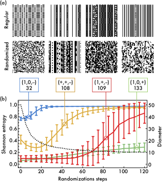
Figure 1: Rules $(1,0,-)$, $(+,+,-)$, $(1,+,-)$, and $(1,0,+)$ (in ECA terms 37, 108, 109, and 133), on graphs with $N=100$ nodes and $d=2$. (a) The upper row shows patterns from a regular ECA architecture, the lower row from randomized counterparts. Time runs downwards. (b) The Shannon entropy $S$ changes differently for every one of the four rules (colored lines) under randomization and is not trivially correlated with the variation of the diameter of the graph (dotted black line), as a prominent topological observable. The results are qualitatively independent of the network size.

Which of these 34 rules are topologically sensitive? That is, which lead to patterns of considerably different complexity when implemented on the regular ECA grid and the RBN architecture? Wolfram classified CA heuristically according to the complexity of the emerging patterns into the four Wolfram classes Wolfram (1984). On graphs, this classification inevitably fails because of a lacking natural node order. Instead, we apply two entropy-like measures, the Shannon entropy $S$ and the word entropy $W$, which we have previously shown to provide a feasible framework for the quantification of pattern complexity Marr and Hütt (2006, 2005); Marr et al. (2007). The Shannon entropy $S$ serves as a measure for the homogeneity of the spatio-temporal pattern, by averaging over all nodes: $S=\frac{1}{N}\sum_{i=1}^{N}-(p^{0}_{i}\log_{2}p^{0}_{i}+p^{1}_{i}\log_{2}p^{1}_{i})$. The probabilities $p^{0}_{i}$ and $p^{1}_{i}$ denote the ratios of 0’s and 1’s in the time series of node $i$. The word entropy $W$ serves as a complexity measure beyond single time steps. It quantifies the irregularity of a time series by counting the number of words, i.e. blocks of constant states confined by the respective different state: $W=\frac{1}{N}\sum_{i=1}^{N}\left(-\sum_{l=1}^{t}p_{i}^{l}\log_{2}p_{i}^{l}\right)$. The probability $p_{i}^{l}$ is the number of words of length $l$ divided by the number of all words found in the time series of node $i$. The maximal possible word length is given by the length $t$ of the time series analyzed.

We compare $10^{3}$ random initial conditions on the regular architecture with $10^{3}$ samples of a randomized graph, where the number of incoming and outgoing links of every node is preserved and kept to $d=2$, but the link architecture has been randomized Trusina et al. (2004). Notably, for a considerably large number of randomization steps, we generate random regular graphs Wormald (1999) rather than Poisson-distributed random graphs Erdős and Rényi (1959).

We classify rules as topologically sensitive, if the difference of the mean entropies for regular and randomized architectures is beyond the standard deviation of the difference. Out of the 34 rules, 14 rules fulfill that condition for at least one observable, $S$ or $W$. These can be divided into three groups: (1) For some rules, the ratio of constant and oscillating nodes changes under randomization, but complex or chaotic patterns never occurs. (2) Others exhibit chaotic patterns on both topologies, but the amount of complexity varies. (3) The most interesting rules are those, for which the change of topology leads to a fundamental change in the complexity of the resulting patterns, i.e., a change in the Wolfram class. These rules are $(1,0,-)$, $(+,+,-)$, $(1,+,-)$, and $(1,0,+)$ (in ECA terms rules 37, 108, 109, and 133). Typical time evolutions of these four rules on regular and random architectures are shown in Figure 1(a). Moreover, these four rules react specifically to topological changes. Figure 1(b) shows the Shannon entropy against the number of randomization steps performed. While the patterns of rules $(1,0,-)$ and $(+,+,-)$ change already when a small number of shortcuts are introduced into the system, $(1,+,-)$ stays constant in this regime but shows higher $S$ and large variations for strongly disordered topologies. Finally, the Shannon entropy of the patterns emerging from rule $(1,0,+)$ grows monotonously with the randomization depth.

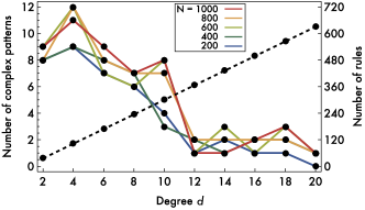
Figure 2: Number of complex patterns (solid colored lines) and number of rules (dashed line) for regular graphs of different networks size against degree $d$. The absolute number of possible rules increases due to the enlarged possible set of $\kappa$ values. Strikingly, the number of single threshold rules with complex patterns is maximal at $d=4$.

Regular graphs—How much complexity is possible on regular graphs? With growing neighborhood size $d$, the number of possible densities $\rho$ and therefore the number of possible rules increases. For the sake of simplicity, we restrict our investigation to a binary state space and to rules with a single threshold: $\kappa$:

$$x_{i}(t+1)=\begin{cases}\alpha\,,&\rho_{i}<\kappa\\ \beta\,,&\rho_{i}=\kappa\\ \gamma\,,&\rho_{i}>\kappa\end{cases}$$ (2)

For networks with $d=12$, 11 different threshold parameters $\kappa\in\{1/12,2/12,\ldots,11/12\}$ lead to 336 different rules, where symmetric rules are considered only once. To estimate the number of rules with complex (that is in our context: non-trivial) patterns, we calculate $W$ for time evolutions. The word entropy is a feasible complexity measure for individual time evolutions. It however fails to disentangle periodic patterns (Wolfram class II) from complex (Wolfram class IV) ones. We therefore supplement our classification with a detrended fluctuation analysis (DFA) Peng et al. (1994). This method characterizes the time correlations of a signal with a single scaling exponent, by calculating the variance of the signal from its trend in a time window for different window sizes. The DFA exponent is the slope of the mean variance against the window size and lies between 0.5 and 1.5 for white and Brownian noise, respectively. Applied to the time evolution of the system’s state density $\bar{\rho}(t)=\sum_{i}x_{i}(t)$ as, e.g., in Amaral et al. (2004), it can be used to discriminate stationary and periodic patterns from complex ones. We count patterns as complex, if the DFA exponent is positive and the word entropy $W>1$. However, the exact values of these thresholds do not alter our results qualitatively. As shown in Figure 2, the number of possible rules (dashed line) increases linearly with $d$, while a maximum of complex patterns (full lines) occurs for $d=4$. The striking overall reduction of complexity for neighborhood enlargement, seen as the most dominant effect in Figure 2 can be understood qualitatively from a homogeneity rationale: In the limit of a fully connected graph, all nodes see nearly the same neighborhood and thus follow the same dynamics (see Marr and Hütt (2005) for a more detailed explanation of a corresponding phenomenon).

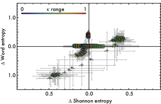
Figure 3: Entropy signature difference plot for 25 scale-free graphs with 200 nodes and 400 links. Both positive and negative entropy differences ($\Delta E=E_{\textrm{H}}-E_{\textrm{R}}$) occur for the comparison of hierarchized vs. randomized graphs.

Complex networks—The formalism of Eq. (2) can be transferred to networks of arbitrary topology. Compared to regular graphs with global neighborhood size $d$, the case where $\rho_{i}=\kappa$ will rarely occur in graphs with heterogeneous connectivity. We thus simplify the set of possible rules with single threshold: By setting $\alpha=\beta$ in Eq. (2), the rule space is condensed and a rule is now defined by the rule parameters $(\alpha,\gamma)$ and the threshold parameter $\kappa$.

As a first exemplary application, we consider scale-free graphs, generated by the incremental Barabási-Albert model Barabási and Albert (1999), with a power law degree distribution, a property often found in real-life networks Albert and Barabási (2002); Newman (2003). Due to their pivotal topological property, the existence of hubs, scale-free graphs have been used frequently as model graphs. They have also been used as a starting point to investigate the relation of degree-degree correlations in complex networks Maslov and Sneppen (2002); Trusina et al. (2004); Weber et al. (2008). Here we want to study how degree correlations in a scale-free graph affect its ability to generate complex patterns. We implement all resulting rules on randomized, hierarchized and anti-hierarchized variants of scale-free graphs with 200 nodes and 400 links. Hierarchization and anti-hierarchization means the gradual randomization towards positive and negative degree-degree correlations, respectively Trusina et al. (2004). For each graph type, we calculate the entropy signatures, given by the Shannon entropy and word entropy of the emerging patterns, for all rules. Figure 3 shows the entropy signature difference plot, where $(S,W)$ of the randomized graphs (R) has been subtracted from the entropy signature of the hierarchized graphs (H), $\Delta E=E_{\textrm{H}}-E_{\textrm{R}}$. Here, $E$ stands for $S$ and $W$ respectively. Most rules are insensitive to degree-degree correlations. Positive and negative entropy signature differences occur preferentially for $(\alpha,\beta)=(+,-)$ or $(\alpha,\beta)=(-,+)$ with $\kappa\in[0.3,0.6]$. Notably, rule $(+,-)$ is a condensed form of the topology-sensitive ECA rule 108, appearing in Figure 1. For the anti-hierarchized graph with negative degree-degree correlations, a similar picture emerges (data not shown).

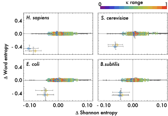
Figure 4: Entropy signature difference plot for the metabolic networks of H. sapiens $(N=625,M=779)$, S. cerevisiae (448, 564), E. coli (563, 709), and B. subtilis (501, 612). $N$ denotes the number of nodes, $M$ the number of links in the largest connected component of the substrate graphs of the respective species. Notably, predominantly negative differences $\Delta S$ and $\Delta W$ occur.

As a second example, we consider the topology of metabolic networks, which abstracts the wiring architecture of the set of enzyme-catalyzed reactions in a specific species. Substrate graphs, where nodes represent metabolites and links represent a reaction between connected substrates can be generated from genomic data Ma and Zeng (2003). In Marr et al. (2007), we recently studied the impact of the topology of metabolic networks on a specific dynamics. There we implemented and studied only a single rule, namely $(+,-)$ as a dynamic probe and interpreted the enhanced regularizing capacity of real networks compared to randomized null models as a possible topological contribution to the reliable establishment of metabolic steady-states and to the effective dampening of fluctuations. To show that the results presented in Marr et al. (2007) are valid over the whole range of dynamics discussed in the present paper, we now implement all possible rules of the form $(\alpha,\gamma)$ on substrate graphs and analyze the entropy signature differences. Figure 4 shows the results for Homo sapiens, Saccharomyces cerevisiae, Escherichia coli, and Bacillus subtilis. We find that while the entropy signatures of most rules do not discriminate between real and randomized topologies, a few rules are topologically sensitive. These rules comply with $(\alpha,\beta)=(+,-)$ or $(\alpha,\beta)=(-,+)$ while $\kappa\in[0.35,0.55]$. For all these rules, the entropy signature of real graphs is significantly smaller compared to the null model topologies. This is also true for hierarchized and anti-hierarchized null models, as well as for all other species investigated in Marr et al. (2007). We believe that the application of dynamic probes is a particularly helpful tool for studying dynamical constraints imposed by topology.

Table 1: Examples of symmetric outer-totalistic CA as defined in Eq. (1), corresponding ECA and RBN rule numbers, as defined in Wolfram (1983) and Kauffman (1969), respectively, and references where these rules have been discussed previously.

Outer-totalistic CA	ECA	RBN	Ref.
$(0,0,0)\leftrightarrow(1,1,1)$	$0\leftrightarrow 255$	$1\leftrightarrow 16$
$(1,0,0)\leftrightarrow(1,1,0)$	$5\leftrightarrow 95$	$2\leftrightarrow 8$	Paul et al. (2006)
$(1,-,+)\leftrightarrow(+,-,0)$	$22\leftrightarrow 151$	-	Matache and Heidel (2004); Nagler and Claussen (2005)
$(0,1,0)\leftrightarrow(1,0,1)$	$90\leftrightarrow 165$	$7\leftrightarrow 10$	Nagler and Claussen (2005)
$(+,+,-)\leftrightarrow(-,+,+)$	$108\leftrightarrow 201$	-	Marr and Hütt (2006, 2005); Marr et al. (2007)
$(+,1,-)\leftrightarrow(-,0,+)$	$126\leftrightarrow 129$	-	Matache and Heidel (2004); Nagler and Claussen (2005)
$(0,0,1)\leftrightarrow(0,1,1)$	$160\leftrightarrow 250$	$9\leftrightarrow 15$	Nochomovitz and Li (2006)
$(0,1,+)\leftrightarrow(+,0,1)$	$164\leftrightarrow 218$	-	Nagler and Claussen (2005)
$(0,+,1)$	$232$	-	Crutchfield and Mitchell (1995); Moreira et al. (2004); Amaral et al. (2004); Nochomovitz and Li (2006)

Discussion—Our formalism can be used to describe outer-totalistic CA and isotropic RBN rules in a common framework. It allows the comprehensive discussion of previously introduced rule sets on diverse topologies, like the selection of Boolean rules presented in Amaral et al. (2004) or variations of the majority rule as used in Moreira et al. (2004); Nochomovitz and Li (2006). It moreover formalizes previous attempts to generalize CA to graphs O’Sullivan (2001); Darabos et al. (2007), and is easily extensible, e.g. by introducing more than just one threshold parameter or by using a larger state space. With the presented framework, the often huge rule space of a discrete dynamical system can be intuitively parametrized and systematically analyzed. The finding of symmetric rules, for example, helps complementing specific CA classes. The set of rules exhibiting power law spectra, as introduced in Nagler and Claussen (2005), can thus be completed with the corresponding symmetric counterparts. Also, many coarse-graining transitions between CA rules, as presented in Israeli and Goldenfeld (2006), can be immediately understood with a symmetry rational. Specific rule generalizations, as discussed and analytically analyzed in Matache and Heidel (2004) may be reconsidered from the more general perspective provided in this letter. As a specific example, the application of ECA rule 22 to arbitrary graphs, stated as an open question in Matache and Heidel (2004), is straightforward with the presented formalism. Limitations arise as soon as individual node characteristics are to be taken into account. Still, the isotropic subset of canalyzing Boolean rules, as discussed in Paul et al. (2006), can be represented with our approach. Table 1 shows some examples of symmetric rules in our formalism, the corresponding ECA and RBN rule number and references where these rules have been previously applied.

An analysis of topologically sensitive rules with analytical tools as developed in Drossel et al. (2005) or the recently introduced basin entropy Krawitz and Shmulevich (2007) may reveal state space changes associated with topological modifications. Such analyses can elucidate dynamic properties also relevant for regulatory dynamics of biological networks, which have been successfully modeled with CA approaches Bornholdt and Sneppen (2000); Li et al. (2004); Davidich and Bornholdt (2008). From this perspective, our framework provides a means to comprehensively study the sensitivity of a system to topological perturbations and associated rule space modifications.

References

- von Neumann (2001) J. von Neumann, in J. von Neumann, Collected Works, edited by A. H. Taub (Macmillan, New York, 2001), vol. 5, p. 288.
- Wolfram (1983) S. Wolfram, Rev. Mod. Phys. 55, 601 (1983).
- Deutsch and Dormann (2005) A. Deutsch and S. Dormann, Cellular Automaton Modeling and Biological Pattern Formation (Birkhäuser, Boston, 2005).
- Kauffman (1969) S. A. Kauffman, J. Theor. Biol. 22, 437 (1969).