The Hilbert Series of Adjoint SQCD

Abstract:

We use the plethystic exponential and the Molien–Weyl formula to compute the Hilbert series (generating functions), which count gauge invariant operators in ${\cal N}=1$ supersymmetric $SU(N_{c})$, $Sp(N_{c})$, $SO(N_{c})$ and $G_{2}$ gauge theories with 1 adjoint chiral superfield, fundamental chiral superfields, and zero classical superpotential. The structure of the chiral ring through the generators and relations between them is examined using the plethystic logarithm and the character expansion technique. The palindromic numerator in the Hilbert series implies that the classical moduli space of adjoint SQCD is an affine Calabi–Yau cone over a weighted projective variety.

1 Introduction and Summary

The rich structures of ${\cal N}=1$ Supersymmetric Quantum Chromodynamics (SQCD) chiral rings and moduli spaces has been studied in [1, 2] using the Plethystic Programme [3, 4, 5, 6, 7, 8, 9, 10], Molien–Weyl formula [11, 12, 13, 14, 15], and character expansions [9, 10, 16]. We can generalise this theory in an interesting way by adding to it a chiral superfield $\phi$ in the adjoint representation, and use the name termed in the literature, ${\cal N}=1$ adjoint SQCD. In this paper, we shall focus on the theory with the $SU(N_{c})$, $Sp(N_{c})$, $SO(N_{c})$ and $G_{2}$ gauge groups with vanishing classical superpotential.

There have been a series of works [17, 18, 19, 20, 21, 22] on the $SU(N_{c})$ adjoint SQCD, as well as [23, 24] on the $SO(N_{c})$ and $Sp(N_{c})$ theories with various classical superpotentials. It is known that the classical moduli space of the $SU(N_{c})$ theory does not get quantum corrections [19, 20, 21]. However, due to technical difficulties, many aspects (e.g., Seiberg duality) of the zero classical superpotential theories have yet to be fully understood. The main aim of this paper is to examine the structure of the chiral rings of adjoint SQCD (with zero superpotential) through the generators of the gauge invariant operators (GIOs) and their relations.

We use the plethystic exponential and the Molien–Weyl formula to obtain Hilbert series, which count GIOs. The generators and the relations in the chiral ring can be extracted from the plethystic logarithm of the Hilbert series. Using the character expansion technique, we can also figure out how these generators and relations transform under the global symmetry.

Hilbert series also contain information about geometrical properties of the moduli space. We shall see in subsequent sections, for example, that plethystic logarithms of Hilbert series can indicate whether the moduli space is a complete intersection, and that the palindomic property of the Hilbert series implies that the moduli space is Calabi–Yau [1, 2, 16].

Below, we collect the main results of our work.

Outline and key points.

• In Section 2, we summarise the Plethystic Programme and Molien–Weyl formula.

• In Section 4, Hilbert series of adjoint SQCD with $SU(N_{c})$ gauge group are constructed. We analyse the generators and relations using the plethystic logarithm. We find that the total number of generators in $SU(N_{c})$ theory with $N_{f}$ flavours is of order $N_{f}^{N_{c}}$.

  • In Subsection 4.2, we count adjoint baryons in the $SU(N_{c})$ theory. This leads to an interesting combinatorial problem of partitions. We find an exponentially large number of adjoint baryons when $N_{c}$ is large. The asymptotic formula is given by (4.46).

  • In Subsection 4.3, the canonical free energy of the theory is derived and found to be of order $N_{f}N_{c}$.

  • In Subsection 4.4, we focus on the complete intersection moduli space of the $SU(N_{c})$ theory (i.e., with 1 flavour). There is exactly one basic relation in this case. A general expression of such a relation for any $N_{c}$ is given by (4.57).

• The structures of generators and relations of the $Sp(N_{c})$, $SO(N_{c})$ and $G_{2}$ adjoint SQCD are studied using Hilbert series in Sections 5, 6, and 7. It is found that $Sp(N_{c})$ theories with 1 flavor, and $SO(N_{c})$ theories with 2 flavors have a moduli space which is a complete intersection, while the moduli space of $SO(N_{c})$ theories with 1 flavor is freely generated. The number of relations for the complete intersection cases is equal to the rank of the gauge group and not to 1 as in the case of $SU(N_{c})$ with 1 flavor.

• In Section 8, we take a geometric aperçu of the moduli space of adjoint SQCD. We establish that the classical moduli space is an irreducible affine Calabi–Yau cone.

Notation for representations.

In this paper, we represent an irreducible representation of a group $G$ by its highest weight $[a_{1},\ldots,a_{r}]$, where $r=\mathrm{rank}~{}G$. Young diagrams are also used in order to avoid cluttered notation. We also slightly abuse terminology by referring to each character by its corresponding representation.

2 Plethystic Programme and Molien–Weyl Formula:
A Recapitulation

In order to write down explicit formulae and for performing computations we need to introduce weights for the different elements in the maximal torus of the different groups. We use

• $z_{a}$ (with $a=1,\ldots,\mathrm{rank}~{}G$) to denote ‘colour’ weights, i.e. coordinates of the maximal torus of the gauge group $G$ ;
  

• $t_{i}$ (with $i=1,\ldots,N_{f}$) to denote ‘flavour’ weights for the fundamental chiral superfield $Q$, i.e. coordinates of the maximal torus of the global $U(N_{f})_{1}$ symmetry ;
  

• $\tilde{t}_{i}$ (with $i=1,\ldots,N_{f}$) to denote ‘flavour’ weights for the antifundamental chiral superfield $\widetilde{Q}$, i.e. coordinates of the maximal torus of the global $U(N_{f})_{2}$ symmetry ;
  

• $s$ to count the chiral superfield $\phi$ in the adjoint representation.

These weights have the interpretation of fugacities for the charges they count and the characters of the representations are functions of these variables. Henceforth, we shall take $t_{i},\>\tilde{t}_{i},\>s$ to be complex variables such that their absolute values lie between 0 and 1.

Below we summarise important facts and conventions of the gauge groups and their Lie algebras which we shall use later [25]:

The group $SU(N_{c})$.

Let us take the weights of the fundamental representation of $SU(N_{c})$ to be

$$L_{1}=(1,0,\ldots,0)~{},\quad L_{k}=(0,0,\ldots,-1,1,\ldots 0)~{},\quad L_{N_{c}}=(0,\ldots,-1)~{},$$ (2.1)

where all $L$’s are $(N_{c}-1)$-tuples, and for $L_{k}$ (with $2\leq k\leq N_{c}-1$), we have $-1$ in the $(k-1)$-th position and $1$ in the $k$-th position. With this choice of weights, we find that the characters of the fundamental and antifundamental representations of $SU(N_{c})$ are

$$[1,0,\ldots,0]_{SU(N_{c})}(z_{a}) = z_{1}+\sum_{k=2}^{N_{c}-1}\frac{z_{k}}{z_{k-1}}+\frac{1}{z_{N_{c}-1}}~{},$$

$$\left[0,\ldots,0,1\right]_{SU(N_{c})}(z_{a}) = \frac{1}{z_{1}}+\sum_{k=2}^{N_{c}-1}\frac{z_{k-1}}{z_{k}}+z_{N_{c}-1}~{}.$$ (2.2)

The roots of the Lie algebra of $SU(N_{c})$ are $\{L_{a}-L_{b}\}_{a\neq b}$. The character of the adjoint representation can be written as

$$\left[1,0,\ldots,0,1\right]_{SU(N_{c})} = [1,0,\ldots,0]_{SU(N_{c})}\times\left[0,\ldots,0,1\right]_{SU(N_{c})}-1$$ (2.3)

$$= (N_{c}-1)+\sum_{\alpha}\left(\prod_{l=1}^{N_{c}-1}z_{l}^{\alpha_{l}}\right)~{},$$

where the summation is taken over all roots $\alpha$, and the notation $\alpha_{l}$ denotes the number in the $l$-th position of the root $\alpha$. For example,

$$[1,1]_{SU(3)}=2+\frac{z_{1}}{z_{2}^{2}}+\frac{1}{z_{1}z_{2}}+\frac{z_{1}^{2}}{z_{2}}+\frac{z_{2}}{z_{1}^{2}}+z_{1}z_{2}+\frac{z_{2}^{2}}{z_{1}}~{}.$$ (2.4)

The group $SO(N_{c})$.

We note that a special orthogonal group falls into one of the two categories of the classical groups, namely $B_{n}=SO(2n+1)$ and $D_{n}=SO(2n)$. The Lie algebras of $B_{n}$ and $D_{n}$ both have the same rank $n$. The weights of the fundamental (vector) representations of $B_{n}$ and $D_{n}$ are respectively $\{0,\pm L_{a}\}$ and $\{\pm L_{a}\}$. With this choice, we can write down the characters of the fundamental representations of $B_{n}$ and $D_{n}$ respectively as

$$\left[1,0,\ldots,0\right]_{B_{n}}(z_{a}) = 1+\sum_{a=1}^{n}\left(z_{a}+\frac{1}{z_{a}}\right)~{},$$

$$\left[1,0,\ldots,0\right]_{D_{n}}(z_{a}) = \sum_{a=1}^{n}\left(z_{a}+\frac{1}{z_{a}}\right)~{}.$$ (2.5)

The adjoint representation of $B_{n}$ and $D_{n}$ is the antisymmetric square of the corresponding fundamental representation: $\mathrm{Adj}_{B_{n},D_{n}}=\Lambda^{2}[1,0,\ldots,0]_{B_{n},D_{n}}$, and so its character is given by

$$\mathrm{Adj}_{B_{n},D_{n}}(z_{a})=\frac{1}{2}\Big{(}\left([1,0,\ldots,0]_{B_{n},D_{n}}(z_{a})\right)^{2}-[1,0,\ldots,0]_{B_{n},D_{n}}(z_{a}^{2})\Big{)}~{}.$$ (2.6)

The roots of the Lie algebras of $B_{n}$ and $D_{n}$ are respectively $\{\pm L_{a}\pm L_{b},\>\pm L_{a}\}_{a\neq b}$ and $\{\pm L_{a}\pm L_{b}\}_{a\neq b}$.

The group $Sp(N_{c})$.

We shall use the notation such that the rank of the Lie algebra of $Sp(N_{c})$ is $N_{c}$, the fundamental representation of $Sp(N_{c})$ is $2N_{c}$ dimensional, and $Sp(1)$ is isomorphic to $SU(2)$. We define $L_{a}=(0,\ldots,0,1_{a;L},0,\ldots,0)$, where the length of the tuple is $N_{c}$. The weights of the fundamental representation are $\{\pm L_{m}\}$. With this choice of $L$’s, we find the character of the fundamental representation to be

$$[1,0,\ldots,0]_{Sp(N_{c})}(z_{a})=\sum_{a=1}^{N_{c}}\left(z_{a}+\frac{1}{z_{a}}\right)~{}.$$ (2.7)

The adjoint representation of $Sp(2N_{c})$ is the symmetric square of the fundamental representation: $\mathrm{Adj}_{Sp(N_{c})}=\mathrm{Sym}^{2}[1,0,\ldots,0]_{Sp(N_{c})}$, and so its character is given by

$$\mathrm{Adj}_{Sp(N_{c})}(z_{a})=\frac{1}{2}\Big{(}\left([1,0,\ldots,0]_{Sp(N_{c})}(z_{a})\right)^{2}+[1,0,\ldots,0]_{Sp(N_{c})}(z_{a}^{2})\Big{)}~{}.$$ (2.8)

The roots of the Lie algebra of $Sp(N_{c})$ are $\{\pm L_{a}\pm L_{b}\}$, where $1\leq a,\>b\leq N_{c}$.

The group $G_{2}$.

The Lie algebra of $G_{2}$ has rank 2. We define $L_{1}=(2,-1),\>L_{2}=(-1,1)$. The weights of the fundamental representation are $\{0,\>\pm L_{1},\>\pm L_{2},\>\pm(L_{1}+L_{2})\}$. With this choice of weights, the character of the fundamental representation is

$$[1,0]_{G_{2}}=1+\frac{1}{z_{1}}+z_{1}+\frac{z_{1}}{z_{2}}+\frac{z_{1}^{2}}{z_{2}}+\frac{z_{2}}{z_{1}^{2}}+\frac{z_{2}}{z_{1}}~{}.$$ (2.9)

The adjoint representation $[0,1]_{G_{2}}$ is given by

$$[0,1] = \Lambda^{2}[1,0]_{G_{2}}-[1,0]_{G_{2}}$$ (2.10)

$$= 2+\frac{1}{z_{1}}+z_{1}+\frac{z_{1}^{3}}{z_{2}^{2}}+\frac{1}{z_{2}}+\frac{z_{1}}{z_{2}}+\frac{z_{1}^{2}}{z_{2}}+\frac{z_{1}^{3}}{z_{2}}+z_{2}+\frac{z_{2}}{z_{1}^{3}}+\frac{z_{2}}{z_{1}^{2}}+\frac{z_{2}}{z_{1}}+\frac{z_{2}^{2}}{z_{1}^{3}}~{}.$$

The plethystic exponential.

The chiral GIOs are symmetric functions of the fundamental chiral superfields $Q^{i}_{a}$, the antifundamental chiral superfields $\widetilde{Q}^{a}_{i}$, and the adjoint chiral superfield $\phi$ which transform respectively in the fundamental, the antifundamental, and the adjoint representations of the gauge group $G$. A convenient combinatorial tool which constructs symmetric products of representations is the plethystic exponential [1, 2, 3, 4, 5, 6, 7, 8, 9, 10], which is a generator for symmetrisation. To briefly remind the reader, we define the plethystic exponential of a multi-variable function $g(t_{1},\ldots,t_{n})$ that vanishes at the origin, $g(0,\ldots,0)=0$, to be

$$\mathrm{PE}[g(t_{1},\ldots,t_{n})]:=\exp\left(\sum_{r=1}^{\infty}\frac{g(t_{1}^{r},\ldots,t_{n}^{r})}{r}\right)~{}.$$ (2.11)

Using formula (2.11) and the expansion $-\log(1-x)=\sum_{k=1}^{\infty}x^{k}/k$, we have, for example,

$$\mathrm{PE}\>\left[[1,0,\ldots,0]_{SU(N_{c})}\sum_{i=1}^{N_{f}}t_{i}\right] = \frac{1}{\prod_{i=1}^{N_{f}}\left[\left(1-t_{i}z_{1}\right)\left(1-\frac{t_{i}}{z_{N_{c}-1}}\right)\prod_{k=2}^{N_{c}-1}(1-t_{i}\frac{z_{k}}{z_{k-1}})\right]}~{},$$

$$\mathrm{PE}\>\left[[1,0,\ldots,0]_{B_{n}}\sum_{i=1}^{N_{f}}t_{i}\right] = \frac{1}{\prod_{i=1}^{N_{f}}\prod_{a=1}^{n}(1-t_{i})(1-t_{i}z_{a})\left(1-\frac{t_{i}}{z_{a}}\right)}~{},$$

$$\mathrm{PE}\>\left[[1,0,\ldots,0]_{D_{n}}\sum_{i=1}^{N_{f}}t_{i}\right] = \frac{1}{\prod_{i=1}^{N_{f}}\prod_{a=1}^{n}(1-t_{i}z_{a})\left(1-\frac{t_{i}}{z_{a}}\right)}~{}.$$ (2.12)

The Molien–Weyl formula.

We emphasize that, in order to obtain the generating function that counts gauge invariant quantities, we need to project the representations of the gauge group generated by the plethystic exponential onto the trivial subrepresentation, which consists of the quantities invariant under the action of the gauge group. Using knowledge from representation theory, this can be done by integrating over the whole group. Hence, the generating function for the gauge group $G$ with $N_{f}$ chiral multiplets in the fundamental representation, $N_{f}$ chiral multiplets in the anitfundamental representaton, and 1 chiral multiplet in the adjoint representation is given by

$$g^{(N_{f},G)}=\int_{G}\mathrm{d}\mu_{G}\>\mathrm{PE}\>\left[\chi^{\text{fund}}_{G}(z_{a})\sum_{i=1}^{N_{f}}t_{i}+\chi^{\text{antifund}}_{G}(z_{a})\sum_{i=1}^{N_{f}}\tilde{t}_{i}+\chi^{\text{adjoint}}_{G}(z^{a})s\right]~{},$$ (2.13)

where the notation $\chi$ signifies the character. This formula is called the Molien–Weyl formula [1, 2, 11, 12, 13, 14, 15]. In the following section, we shall demonstrate in details how to use this formula to count GIOs. We note that the Haar measure for the gauge group $\mu_{G}$ is given by [26]

$$\int_{G}\mathrm{d}\mu_{G}=\frac{1}{(2\pi i)^{r}}\oint_{|z_{1}|=1}\ldots\oint_{|z_{r}|=1}\frac{\mathrm{d}z_{1}}{z_{1}}\ldots\frac{\mathrm{d}z_{r}}{z_{r}}\prod_{\alpha^{+}}\left(1-\prod_{l=1}^{r}z_{l}^{\alpha^{+}_{l}}\right)~{},$$ (2.14)

where $\alpha^{+}$ are positive roots of the Lie algebra of the gauge group $G$ and $r=\mathrm{rank}~{}G$. For example,

$$\int_{SU(2)}\mathrm{d}\mu_{SU(2)} = \frac{1}{2\pi i}\oint_{|z|=1}\frac{dz}{z}(1-z^{2})~{},$$

$$\int_{SU(3)}\mathrm{d}\mu_{SU(3)} = \frac{1}{(2\pi i)^{2}}\oint_{|z_{1}|=1}\frac{dz_{1}}{z_{1}}\oint_{|z_{2}|=1}\frac{dz_{2}}{z_{2}}\left(1-z_{1}z_{2}\right)\left(1-\frac{z^{2}_{1}}{z_{2}}\right)\left(1-\frac{z^{2}_{2}}{z_{1}}\right)~{},$$

$$\int_{SO(3)}\mathrm{d}\mu_{SO(3)} = \frac{1}{2\pi i}\oint_{|z|=1}\frac{\mathrm{d}z}{z}\left(1-z\right)~{},$$

$$\int_{SO(4)}\mathrm{d}\mu_{SO(4)} = \frac{1}{(2\pi i)^{2}}\oint_{|z_{1}|=1}\frac{\mathrm{d}z_{1}}{z_{1}}\oint_{|z_{2}|=1}\frac{\mathrm{d}z_{2}}{z_{2}}\left(1-\frac{z_{1}}{z_{2}}\right)(1-z_{1}z_{2})~{},$$

$$\int_{SO(5)}\mathrm{d}\mu_{SO(5)} = \frac{1}{(2\pi i)^{2}}\oint_{|z_{1}|=1}\frac{\mathrm{d}z_{1}}{z_{1}}\oint_{|z_{2}|=1}\frac{\mathrm{d}z_{2}}{z_{2}}(1-z_{1})(1-z_{2})\left(1-\frac{z_{1}}{z_{2}}\right)(1-z_{1}z_{2})~{},$$

$$\int_{Sp(2)}\mathrm{d}\mu_{Sp(2)} = \frac{1}{(2\pi i)^{2}}\oint_{|z_{1}|=1}\frac{\mathrm{d}z_{1}}{z_{1}}\oint_{|z_{2}|=1}\frac{\mathrm{d}z_{2}}{z_{2}}(1-z_{1}^{2})(1-z_{2})(1-\frac{z_{1}^{2}}{z_{2}})(1-\frac{z_{2}^{2}}{z_{1}^{2}})~{},$$

$$\int_{G_{2}}\mathrm{d}\mu_{G_{2}} = \frac{1}{(2\pi i)^{2}}\oint_{|z_{1}|=1}\frac{\mathrm{d}z_{1}}{z_{1}}\oint_{|z_{2}|=1}\frac{\mathrm{d}z_{2}}{z_{2}}\left(1-z_{1}\right)\left(1-\frac{z_{1}^{2}}{z_{2}}\right)\left(1-\frac{z_{1}^{3}}{z_{2}}\right)\left(1-z_{2}\right)\times$$ (2.15)

$$\left(1-\frac{z_{2}}{z_{1}}\right)\left(1-\frac{z_{2}^{2}}{z_{1}^{3}}\right)~{}.$$

The Hilbert series.

A Hilbert series is a function that counts chiral gauge invariant operators and has the interpretation of a partition function at zero temperature and non-zero chemical potentials for global conserved $U(1)$ charges. It can be written as a rational function whose numerator is a polynomial with integer coefficients. Importantly, the powers of the denominators are such that the leading pole captures the dimension of the manifold.

The plethystic logarithm.

Information about the generators of the moduli space and the relations they satisfy can be computed by using the plethystic logarithm [1, 2, 3, 5, 6, 9, 16], which is the inverse function of the plethystic exponential. Using the Möbius function $\mu(r)$ we define:

$$\mathrm{PL}[g(t_{1},\ldots,t_{n})]:=\sum_{r=1}^{\infty}\frac{\mu(r)\log g(t_{1}^{r},\ldots,t_{n}^{r})}{r}~{}.$$ (2.16)

The significance of the series expansion of the plethystic logarithm is that the first terms with plus sign give the basic generators while the first terms with the minus sign give the constraints between these basic generators. If the formula (2.16) is an infinite series of terms with plus and minus signs, then the moduli space is not a complete intersection and the constraints in the chiral ring are not trivially generated by relations between the basic generators, but receive stepwise corrections at higher degree. These are the so-called higher syzygies.

3 Dimension of the Moduli Space

At a generic point of the moduli space, the gauge symmetry $G$ is broken completely, and hence there are $d(G)$ broken generators. In the Higgs mechanism, a massless vector multiplet ‘eats’ an entire chiral multiplet to form a massive vector multiplet. Originally, we have $d(G)$ degrees of freedom coming from the chiral superfields in the adjoint representation (which is $d(G)$ dimensional), and $N_{\chi}d(\Box)$ degrees of freedom coming from the $N_{\chi}$ chiral superfields in the fundamental (and antifundamental) representation (which is $d(\Box)$ dimensional). Therefore, of the original $d(G)+N_{\chi}d(\Box)$ chiral degrees of freedom, only $\left[d(G)+N_{\chi}d(\Box)\right]-d(G)=N_{\chi}d(\Box)$ singlets are left massless. Therefore, the dimension of the moduli space ${\cal M}$ is

$$\dim{\cal M}=N_{\chi}d(\Box)~{}.$$ (3.1)

For the $SU(N_{c})$ adjoint SQCD with $N_{f}$ chiral superfields in the fundamental representation and $N_{f}$ chiral superfields in the antifundamental representation, we have $N_{\chi}=2N_{f}$ and $d(\tiny{\Box})=N_{c}$. Therefore,

$$\dim{\cal M}_{(N_{f},SU(N_{c}))}=2N_{f}N_{c}~{}.$$ (3.2)

For the $Sp(N_{c})$ adjoint SQCD with $2N_{f}$ chiral superfields in the fundamental representation, we have $N_{\chi}=2N_{f}$ and $d(\tiny{\Box})=2N_{c}$. Therefore,

$$\dim{\cal M}_{(N_{f},Sp(N_{c}))}=4N_{f}N_{c}~{}.$$ (3.3)

For the $SO(N_{c})$ adjoint SQCD with $N_{f}$ chiral superfields in the fundamental (vector) representation, we have $N_{\chi}=N_{f}$ and $d(\tiny{\Box})=N_{c}$. Therefore,

$$\dim{\cal M}_{(N_{f},SO(N_{c}))}=N_{f}N_{c}~{}.$$ (3.4)

For the $G_{2}$ adjoint SQCD with $N_{f}$ chiral superfields in the fundamental representation, we have $N_{\chi}=N_{f}$ and $d(\tiny{\Box})=7$. Therefore,

$$\dim{\cal M}_{(N_{f},G_{2})}=7N_{f}~{}.$$ (3.5)

4 The $SU(N_{c})$ Gauge Groups

Let us consider the $SU(N_{c})$ theory with $N_{f}$ chiral superfields transforming in the fundamental representation, $N_{f}$ chiral superfields transforming in the antifundamental representation (i.e. $N_{f}$ flavours), and 1 chiral superfield transforming in the adjoint representation. The anomaly-free global symmetry of this theory [19] is $SU(N_{f})\times SU(N_{f})\times U(1)_{B}\times U(1)_{R_{1}}\times U(1)_{R_{2}}$.

4.1 Examples of Hilbert Series

Below we shall derive Hilbert series for various cases.

4.1.1 The $SU(2)$ Gauge Group

We start the analysis by the simplest case of the $SU(2)$ gauge theory with $2N_{f}$ chiral superfields transforming in the fundamental representation ($N_{f}$ flavours) and 1 chiral multiplet transforming in the adjoint representation. The Molien–Weyl formula can be written explicitly as:

$$g^{(N_{f},SU(2))}(s,t) = \frac{1}{2\pi i}\oint_{|z|=1}\frac{dz}{z}(1-z^{2})~{}\mathrm{PE}\>\left[2N_{f}[1]t+[2]s\right]$$

$$= \frac{1}{2\pi i}\oint_{|z|=1}\frac{dz}{z}\frac{1-z^{2}}{(1-tz)^{2N_{f}}(1-\frac{t}{z})^{2N_{f}}(1-s)(1-sz^{2})(1-\frac{s}{z^{2}})}~{}.$$

Noting that $0<|t|,|s|<1$, we use the residue theorem with the poles $z=t,\>\sqrt{s},-\sqrt{s}$ and find that

$$g^{(1,SU(2))}(s,t) = \frac{1+st^{2}}{(1-s^{2})(1-t^{2})(1-st^{2})^{2}}$$

$$= 1+s^{2}+s^{4}+t^{2}+3st^{2}+s^{2}t^{2}+3s^{3}t^{2}+s^{4}t^{2}+3s^{5}t^{2}+t^{4}+3st^{4}+6s^{2}t^{4}+$$

$$3s^{3}t^{4}+6s^{4}t^{4}+3s^{5}t^{4}+O(s^{6})O(t^{6})~{},$$

$$g^{(2,SU(2))}(s,t) = \frac{1+t^{2}+6st^{2}-9st^{4}+s^{2}t^{4}+st^{6}-9s^{2}t^{6}+6s^{2}t^{8}+s^{3}t^{8}+s^{3}t^{10}}{(1-s^{2})(1-t^{2})^{5}(1-st^{2})^{4}}$$

$$= 1+s^{2}+s^{4}+6t^{2}+10st^{2}+6s^{2}t^{2}+10s^{3}t^{2}+6s^{4}t^{2}+10s^{5}t^{2}+20t^{4}+$$

$$45st^{4}+55s^{2}t^{4}+45s^{3}t^{4}+55s^{4}t^{4}+45s^{5}t^{4}+O(s^{6})O(t^{6})~{},$$

$$g^{(3,SU(2))}(s,t) = 1+s^{2}+s^{4}+15t^{2}+21st^{2}+15s^{2}t^{2}+21s^{3}t^{2}+15s^{4}t^{2}+21s^{5}t^{2}+105t^{4}+$$

$$210st^{4}+231s^{2}t^{4}+210s^{3}t^{4}+231s^{4}t^{4}+210s^{5}t^{4}+O(s^{6})O(t^{6})~{},$$

$$g^{(4,SU(2))}(s,t) = 1+s^{2}+s^{4}+28t^{2}+36st^{2}+28s^{2}t^{2}+36s^{3}t^{2}+28s^{4}t^{2}+36s^{5}t^{2}+336t^{4}+$$

$$630st^{4}+666s^{2}t^{4}+630s^{3}t^{4}+666s^{4}t^{4}+630s^{5}t^{4}+O(s^{6})O(t^{6})~{},$$

$$g^{(5,SU(2))}(s,t) = 1+s^{2}+s^{4}+45t^{2}+55st^{2}+45s^{2}t^{2}+55s^{3}t^{2}+45s^{4}t^{2}+55s^{5}t^{2}+825t^{4}+$$ (4.2)

$$1485st^{4}+1540s^{2}t^{4}+1485s^{3}t^{4}+1540s^{4}t^{4}+1485s^{5}t^{4}+O(s^{6})O(t^{6})~{}.$$

Looking at these generating functions, it is possible to predict the order of the numerator and the terms in the denominator of the generating function for a case with $N_{f}$ fundamental quarks:

$$g^{(N_{f},SU(2))} = \frac{P_{(2N_{f}-1),(8N_{f}-6)}(s,t)}{(1-s^{2})(1-t^{2})^{4N_{f}-3}(1-st^{2})^{2N_{f}}},$$ (4.3)

where $P_{a,b}(s,t)$ is a polynomial of degree $a$ in $s$ and of degree $b$ in $t$. The calculation is simpler when we make a further identification $s=t$. In which case, we can write down a general form of the generating function:

$$g^{(N_{f},SU(2))}(t) = \frac{P_{8N_{f}-6}(t)}{(1+t)^{2N_{f}-3}(1-t^{2})^{2N_{f}}(1-t^{3})^{2N_{f}}}~{},$$ (4.4)

where $P_{8N_{f}-6}(t)$ is a palindromic polynomial of degree $8N_{f}-6$ in $t$ with $P_{8N_{f}-6}(1)\neq 0$ for all $N_{f}$. Observe that the order of the pole at $t=1$ of $g^{(N_{f},SU(2))}(t)$ is $4N_{f}$. Therefore, the dimension of the moduli space ${\cal M}_{(N_{f},SU(2))}$ is $4N_{f}$, in agreement with (3.2) and (3.3).

Character expansion.

We can write down the generating function for an arbitary number of flavous $N_{f}$ in terms of representations of the global symmetry $SU(2N_{f})$ as follows:

$$g^{(N_{f},SU(2))} = \sum^{\infty}_{n_{1}=0}\sum^{\infty}_{n_{2}=0}\sum_{m=0}^{\infty}[2n_{1},n_{2},0,\ldots,0]{s^{n_{1}+2m}t^{2n_{1}+2n_{2}}}$$ (4.5)

$$= \frac{1}{1-s^{2}}\sum^{\infty}_{n_{1}=0}\sum^{\infty}_{n_{2}=0}[2n_{1},n_{2},0,\ldots,0]{s^{n_{1}}t^{2n_{1}+2n_{2}}}~{}.$$

We emphasise that $\frac{1}{1-s^{2}}$ does factor out from the character expansion.

Plethystic logarithms.

We shall calculate the plethystic logarithms of the generating functions in (4.2) using formula (2.16):

$$\mathrm{PL}[g^{(1,SU(2))}(s,t)] = s^{2}+t^{2}+3st^{2}-s^{2}t^{4}~{},$$

$$\mathrm{PL}[g^{(2,SU(2))}(s,t)] = s^{2}+6t^{2}+10st^{2}-t^{4}-15st^{4}-20s^{2}t^{4}+O(s^{6})O(t^{6})~{},$$

$$\mathrm{PL}[g^{(3,SU(2))}(s,t)] = s^{2}+15t^{2}+21st^{2}-15t^{4}-105st^{4}-105s^{2}t^{4}+O(s^{6})O(t^{6})$$

$$\mathrm{PL}[g^{(4,SU(2))}(s,t)] = s^{2}+28t^{2}+36st^{2}-70t^{4}-378st^{4}-336s^{2}t^{4}+O(s^{6})O(t^{6})$$

$$\mathrm{PL}[g^{(5,SU(2))}(s,t)] = s^{2}+45t^{2}+55st^{2}-210t^{4}-990st^{4}-825s^{2}t^{4}+O(s^{6})O(t^{6})~{}.$$

Observe that only plethystic logarithm of $g^{(1,SU(2))}$ is a polynomial. Therefore, the moduli space of the $SU(2)$ gauge theory with 1 flavour and 1 adjoint matter is a complete intersection.

Generators of the GIOs.

According to (4.1.1), we see that there are only 3 types of generators of the GIOs in the $SU(2)$ theory, namely

$$\begin{array}[]{llllll}\mbox{\bf Casimir invariants}:&s^{2}&\rightarrow&u\equiv{\rm Tr}(\phi^{2})&\hbox{:}\quad[0,\ldots,0]&1~{}\text{dimensional}~{},\\ \mbox{\bf Mesons}:&t^{2}&\rightarrow&M^{ij}\equiv\epsilon^{ab}Q^{i}_{a}\>{Q}^{j}_{b}&\hbox{:}\quad[0,1,\ldots,0]&{2N_{f}\choose 2}~{}\text{dimensional}~{},\\ \mbox{\bf Adjoint mesons}:&st^{2}&\rightarrow&A^{ij}\equiv\epsilon^{ab}\epsilon^{cd}Q^{i}_{a}\phi_{bc}\>{Q}^{j}_{d}&\hbox{:}\quad[2,0,\ldots,0]&N_{f}(2N_{f}+1)~{}\text{dimensional}~{}.\end{array}$$

Note that the total number of generators is quadratic in $N_{f}$,

$$1+{2N_{f}\choose 2}+N_{f}(2N_{f}+1)=4N_{f}^{2}+1~{}.$$ (4.7)

Relations between the generators.

From plethystic logarithms (4.1.1), we see that there are 3 types of basic relations:

• Order $t^{4}$: The relations are known from the theory without adjoint:

  $$\mathrm{Pf}~{}M=\epsilon_{i_{1}\ldots i_{2N_{f}}}M^{i_{1}i_{2}}M^{i_{3}i_{4}}=0~{}.$$ (4.8)

  They transform in the $SU(2N_{f})$ representation $[0,0,0,1,0,\ldots,0]$. We note that this is contained in the decomposition of the symmetric square of the representation $[0,1,0,\ldots,0]$ at order $t^{2}$.

• Order $st^{4}$: The relations transform in the representation $[1,0,1,0,\ldots,0]$, which is contained in the decomposition of the antisymmetric product of the representation $[2,0,\ldots,0]$ at order $st^{2}$ and the representation $[0,1,0,\ldots,0]$ at order $t^{2}$.

• Order $s^{2}t^{4}$: The relations transform in the representation $[0,2,0,\ldots,0]$, which is contained in the decomposition of the symmetric square of the representation $[2,0,\ldots,0]$ at order $st^{2}$. In the case of 1 flavour, there is only 1 basic relation which can be written out explicitly as

  $$A^{11}A^{22}-\left(A^{12}\right)^{2}+\frac{1}{2}u\left(M^{12}\right)^{2}=0~{}.$$ (4.9)

In summary, for the $SU(2)$ theory, we have the basic relations which transform in the $SU(2N_{f})$ representations $[0,0,0,1,0,\ldots,0]$, $[1,0,1,0,\ldots,0]$, and $[0,2,0,\ldots,0]$.

Therefore, we may write down a general expression of the plethystic logarithm in terms of $SU(2N_{f})$ representations as

$$\mathrm{PL}[g^{(N_{f},SU(2))}(s,t)] = [0,\ldots,0]s^{2}+[0,1,\ldots,0]t^{2}+[2,0,\ldots,0]st^{2}$$

$$-[0,0,0,1,0,\ldots,0]t^{4}-[1,0,1,0,\ldots,0]st^{4}-[0,2,0,\ldots,0]s^{2}t^{4}+O(s^{6})O(t^{6})~{}.$$

4.1.2 The $SU(3)$ Gauge Group

Now let us turn to the $SU(3)$ theory with $N_{f}$ flavours and 1 adjoint matter. We have $N_{f}$ chiral superfields transforming in the fundamental representation, $N_{f}$ chiral superfields transforming in the antifundamental representation, and 1 chiral superfield transforming in the adjoint representation. Therefore, we can apply the Molien–Weyl formula to our theory as follows:

$$g^{(N_{f},SU(3))} = \frac{1}{(2\pi i)^{2}}\oint\limits_{|z_{1}|=1}\frac{dz_{1}}{z_{1}}\oint\limits_{|z_{2}|=1}\frac{dz_{2}}{z_{2}}\left(1-z_{1}z_{2}\right)\left(1-\frac{z^{2}_{1}}{z_{2}}\right)\left(1-\frac{z^{2}_{2}}{z_{1}}\right)\mathrm{PE}\left[N_{f}[1,0]t+N_{f}[0,1]\tilde{t}+[1,1]s\right]$$ (4.11)

$$= \frac{1}{(2\pi i)^{2}}\oint\limits_{|z_{1}|=1}\frac{dz_{1}}{z_{1}}\oint\limits_{|z_{2}|=1}\frac{dz_{2}}{z_{2}}\frac{\left(1-z_{1}z_{2}\right)\left(1-\frac{z^{2}_{1}}{z_{2}}\right)\left(1-\frac{z^{2}_{2}}{z_{1}}\right)}{\left((1-tz_{1})(1-t\frac{z_{2}}{z_{1}})(1-\frac{t}{z_{2}})\right)^{N_{f}}\left((1-\tilde{t}z_{2})(1-\tilde{t}\frac{z_{1}}{z_{2}})(1-\frac{\tilde{t}}{z_{1}})\right)^{N_{f}}}\times$$

$$\frac{1}{(1-sz_{1}z_{2})(1-s\frac{z^{2}_{1}}{z_{2}})(1-s\frac{z^{2}_{2}}{z_{1}})(1-s\frac{z_{1}}{z^{2}_{2}})(1-s\frac{z_{2}}{z^{2}_{1}})(1-s\frac{1}{z_{1}z_{2}})(1-s)^{2}}~{}.$$

Applying the residue theorem, we have

$$g^{(1,SU(3))}(s,t,\tilde{t}) = \frac{1-s^{6}t^{3}\tilde{t}^{3}}{\left(1-s^{2}\right)\left(1-s^{3}\right)\left(1-t\tilde{t}\right)\left(1-st\tilde{t}\right)\left(1-s^{2}t\tilde{t}\right)\left(1-s^{3}t^{3}\right)\left(1-s^{3}\tilde{t}^{3}\right)}$$

$$= 1+s^{2}+s^{3}+s^{4}+s^{5}+2s^{6}+s^{3}t^{3}+s^{5}t^{3}+s^{6}t^{3}+t\tilde{t}+st\tilde{t}+2s^{2}t\tilde{t}+$$

$$2s^{3}t\tilde{t}+3s^{4}t\tilde{t}+3s^{5}t\tilde{t}+4s^{6}t\tilde{t}+t^{2}\tilde{t}^{2}+st^{2}\tilde{t}^{2}+3s^{2}t^{2}\tilde{t}^{2}+3s^{3}t^{2}\tilde{t}^{2}+$$

$$5s^{4}t^{2}\tilde{t}^{2}+5s^{5}t^{2}\tilde{t}^{2}+7s^{6}t^{2}\tilde{t}^{2}+s^{3}\tilde{t}^{3}+s^{5}\tilde{t}^{3}+s^{6}\tilde{t}^{3}+t^{3}\tilde{t}^{3}+st^{3}\tilde{t}^{3}+$$

$$3s^{2}t^{3}\tilde{t}^{3}+4s^{3}t^{3}\tilde{t}^{3}+6s^{4}t^{3}\tilde{t}^{3}+7s^{5}t^{3}\tilde{t}^{3}+10s^{6}t^{3}\tilde{t}^{3}+O(s^{7})O(t^{4})O(\tilde{t}^{4})~{},$$

$$g^{(2,SU(3))}(s,t,\tilde{t}) = 1+s^{2}+s^{3}+s^{4}+s^{5}+2s^{6}+2st^{3}+2s^{2}t^{3}+6s^{3}t^{3}+4s^{4}t^{3}+8s^{5}t^{3}+8s^{6}t^{3}+$$

$$4t\tilde{t}+4st\tilde{t}+8s^{2}t\tilde{t}+8s^{3}t\tilde{t}+12s^{4}t\tilde{t}+12s^{5}t\tilde{t}+16s^{6}t\tilde{t}+10t^{2}\tilde{t}^{2}+16st^{2}\tilde{t}^{2}+$$

$$35s^{2}t^{2}\tilde{t}^{2}+41s^{3}t^{2}\tilde{t}^{2}+60s^{4}t^{2}\tilde{t}^{2}+66s^{5}t^{2}\tilde{t}^{2}+85s^{6}t^{2}\tilde{t}^{2}+2s\tilde{t}^{3}+2s^{2}\tilde{t}^{3}+$$

$$6s^{3}\tilde{t}^{3}+4s^{4}\tilde{t}^{3}+8s^{5}\tilde{t}^{3}+8s^{6}\tilde{t}^{3}+20t^{3}\tilde{t}^{3}+40st^{3}\tilde{t}^{3}+96s^{2}t^{3}\tilde{t}^{3}+136s^{3}t^{3}\tilde{t}^{3}+$$

$$204s^{4}t^{3}\tilde{t}^{3}+244s^{5}t^{3}\tilde{t}^{3}+316s^{6}t^{3}\tilde{t}^{3}+O(s^{7})O(t^{4})O(\tilde{t}^{4})~{},$$

$$g^{(3,SU(3))}(s,t,\tilde{t}) = 1+s^{2}+s^{3}+s^{4}+s^{5}+2s^{6}+t^{3}+8st^{3}+9s^{2}t^{3}+19s^{3}t^{3}+17s^{4}t^{3}+27s^{5}t^{3}+$$

$$28s^{6}t^{3}+9t\tilde{t}+9st\tilde{t}+18s^{2}t\tilde{t}+18s^{3}t\tilde{t}+27s^{4}t\tilde{t}+27s^{5}t\tilde{t}+36s^{6}t\tilde{t}+$$

$$45t^{2}\tilde{t}^{2}+81st^{2}\tilde{t}^{2}+162s^{2}t^{2}\tilde{t}^{2}+198s^{3}t^{2}\tilde{t}^{2}+279s^{4}t^{2}\tilde{t}^{2}+315s^{5}t^{2}\tilde{t}^{2}+$$

$$396s^{6}t^{2}\tilde{t}^{2}+\tilde{t}^{3}+8s\tilde{t}^{3}+9s^{2}\tilde{t}^{3}+19s^{3}\tilde{t}^{3}+17s^{4}\tilde{t}^{3}+27s^{5}\tilde{t}^{3}+28s^{6}\tilde{t}^{3}+$$

$$165t^{3}\tilde{t}^{3}+404st^{3}\tilde{t}^{3}+893s^{2}t^{3}\tilde{t}^{3}+1301s^{3}t^{3}\tilde{t}^{3}+1881s^{4}t^{3}\tilde{t}^{3}+2289s^{5}t^{3}\tilde{t}^{3}+$$

$$2878s^{6}t^{3}\tilde{t}^{3}+O(s^{7})O(t^{4})O(\tilde{t}^{4})~{},$$

$$g^{(4,SU(3))}(s,t,\tilde{t}) = 1+s^{2}+s^{3}+s^{4}+s^{5}+2s^{6}+4t^{3}+20st^{3}+24s^{2}t^{3}+44s^{3}t^{3}+44s^{4}t^{3}+64s^{5}t^{3}+$$

$$68s^{6}t^{3}+16t\tilde{t}+16st\tilde{t}+32s^{2}t\tilde{t}+32s^{3}t\tilde{t}+48s^{4}t\tilde{t}+48s^{5}t\tilde{t}+64s^{6}t\tilde{t}+$$

$$136t^{2}\tilde{t}^{2}+256st^{2}\tilde{t}^{2}+492s^{2}t^{2}\tilde{t}^{2}+612s^{3}t^{2}\tilde{t}^{2}+848s^{4}t^{2}\tilde{t}^{2}+968s^{5}t^{2}\tilde{t}^{2}+$$

$$1204s^{6}t^{2}\tilde{t}^{2}+4\tilde{t}^{3}+20s\tilde{t}^{3}+24s^{2}\tilde{t}^{3}+44s^{3}\tilde{t}^{3}+44s^{4}\tilde{t}^{3}+64s^{5}\tilde{t}^{3}+68s^{6}\tilde{t}^{3}+$$

$$816t^{3}\tilde{t}^{3}+2160st^{3}\tilde{t}^{3}+4576s^{2}t^{3}\tilde{t}^{3}+6736s^{3}t^{3}\tilde{t}^{3}+9536s^{4}t^{3}\tilde{t}^{3}+11696s^{5}t^{3}\tilde{t}^{3}+$$

$$14512s^{6}t^{3}\tilde{t}^{3}+O(s^{7})O(t^{4})O(\tilde{t}^{4})~{},$$

$$g^{(5,SU(3))}(s,t,\tilde{t}) = 1+s^{2}+s^{3}+s^{4}+s^{5}+2s^{6}+10t^{3}+40st^{3}+50s^{2}t^{3}+85s^{3}t^{3}+90s^{4}t^{3}+125s^{5}t^{3}+$$

$$135s^{6}t^{3}+25t\tilde{t}+25st\tilde{t}+50s^{2}t\tilde{t}+50s^{3}t\tilde{t}+75s^{4}t\tilde{t}+75s^{5}t\tilde{t}+100s^{6}t\tilde{t}+$$

$$325t^{2}\tilde{t}^{2}+625st^{2}\tilde{t}^{2}+1175s^{2}t^{2}\tilde{t}^{2}+1475s^{3}t^{2}\tilde{t}^{2}+2025s^{4}t^{2}\tilde{t}^{2}+2325s^{5}t^{2}\tilde{t}^{2}+$$

$$2875s^{6}t^{2}\tilde{t}^{2}+10\tilde{t}^{3}+40s\tilde{t}^{3}+50s^{2}\tilde{t}^{3}+85s^{3}\tilde{t}^{3}+90s^{4}\tilde{t}^{3}+125s^{5}\tilde{t}^{3}+135s^{6}\tilde{t}^{3}+$$

$$2925t^{3}\tilde{t}^{3}+8025st^{3}\tilde{t}^{3}+16575s^{2}t^{3}\tilde{t}^{3}+24500s^{3}t^{3}\tilde{t}^{3}+34250s^{4}t^{3}\tilde{t}^{3}+42175s^{5}t^{3}\tilde{t}^{3}+$$

$$51950s^{6}t^{3}\tilde{t}^{3}+O(s^{7})O(t^{4})O(\tilde{t}^{4})~{},$$

$$g^{(6,SU(3))}(s,t,\tilde{t}) = 1+s^{2}+s^{3}+s^{4}+s^{5}+2s^{6}+20t^{3}+70st^{3}+90s^{2}t^{3}+146s^{3}t^{3}+160s^{4}t^{3}+216s^{5}t^{3}+$$ (4.12)

$$236s^{6}t^{3}+36t\tilde{t}+36st\tilde{t}+72s^{2}t\tilde{t}+72s^{3}t\tilde{t}+108s^{4}t\tilde{t}+108s^{5}t\tilde{t}+144s^{6}t\tilde{t}+666t^{2}\tilde{t}^{2}+$$

$$1296st^{2}\tilde{t}^{2}+2403s^{2}t^{2}\tilde{t}^{2}+3033s^{3}t^{2}\tilde{t}^{2}+4140s^{4}t^{2}\tilde{t}^{2}+4770s^{5}t^{2}\tilde{t}^{2}+5877s^{6}t^{2}\tilde{t}^{2}+$$

$$20\tilde{t}^{3}+70s\tilde{t}^{3}+90s^{2}\tilde{t}^{3}+146s^{3}\tilde{t}^{3}+160s^{4}\tilde{t}^{3}+216s^{5}\tilde{t}^{3}+236s^{6}\tilde{t}^{3}+8436t^{3}\tilde{t}^{3}+$$

$$23576st^{3}\tilde{t}^{3}+47888s^{2}t^{3}\tilde{t}^{3}+70904s^{3}t^{3}\tilde{t}^{3}+98316s^{4}t^{3}\tilde{t}^{3}+121332s^{5}t^{3}\tilde{t}^{3}+$$

$$148780s^{6}t^{3}\tilde{t}^{3}+O(s^{7})O(t^{4})O(\tilde{t}^{4})~{}.$$

We remark that, although these results seem to be rather lengthy, they contain information which proves to be extremely useful for analyses of the chiral ring. As we shall see from plethystic logarithms, $s^{6}t^{3}\tilde{t}^{3}$ is the minimum order up to which Hilbert series contain all necessary information about the generators and their basic relations.

The calculation is significantly simpler when we make an identification $s=t=\tilde{t}$. In which case, we can write down a general form of the generating function:

$$g^{(N_{f},SU(3))}(t)=\frac{P_{14N_{f}-10}(t)}{(1-t)^{N_{f}-1}(1-t^{2})^{N_{f}+2}(1-t^{3})^{N_{f}+1}(1-t^{4})^{2N_{f}-2}(1-t^{6})^{N_{f}}}~{},$$ (4.13)

where $P_{14N_{f}-10}(t)$ is a palindromic polynomial of degree $14N_{f}-10$ with $P_{14N_{f}-10}(1)$ being a non-zero number for any number of flavour. Observe that the order of the pole at $t=1$ of $g^{(N_{f},SU(3))}(t)$ is $6N_{f}$. Therefore, the dimension of the moduli space ${\cal M}_{(N_{f},SU(3))}$ is $6N_{f}$ in agreement with (3.2).

Plethystic logarithms.

We shall calculate plethystic logarithms of generating functions using formula (2.16):

$$\mathrm{PL}[g^{(1,SU(3))}(s,t,\tilde{t})] = s^{2}+s^{3}+t\tilde{t}+st\tilde{t}+s^{2}t\tilde{t}+s^{3}t^{3}+s^{3}\tilde{t}^{3}-s^{6}t^{3}\tilde{t}^{3}~{},$$

$$\mathrm{PL}[g^{(2,SU(3))}(s,t,\tilde{t})] = s^{2}+s^{3}+2st^{3}+2s^{2}t^{3}+4s^{3}t^{3}+4t\tilde{t}+4st\tilde{t}+4s^{2}t\tilde{t}-s^{2}t^{2}\tilde{t}^{2}-s^{3}t^{2}\tilde{t}^{2}-s^{4}t^{2}\tilde{t}^{2}$$

$$+2s\tilde{t}^{3}+2s^{2}\tilde{t}^{3}+4s^{3}\tilde{t}^{3}-4s^{2}t^{3}\tilde{t}^{3}-8s^{3}t^{3}\tilde{t}^{3}-20s^{4}t^{3}\tilde{t}^{3}-16s^{5}t^{3}\tilde{t}^{3}-16s^{6}t^{3}\tilde{t}^{3}$$

$$+O(s^{7})O(t^{4})O(\tilde{t}^{4})~{},$$

$$\mathrm{PL}[g^{(3,SU(3))}(s,t,\tilde{t})] = s^{2}+s^{3}+t^{3}+8st^{3}+8s^{2}t^{3}+10s^{3}t^{3}+9t\tilde{t}+9st\tilde{t}+9s^{2}t\tilde{t}-9s^{2}t^{2}\tilde{t}^{2}-9s^{3}t^{2}\tilde{t}^{2}$$

$$-9s^{4}t^{2}\tilde{t}^{2}+\tilde{t}^{3}+8s\tilde{t}^{3}+8s^{2}\tilde{t}^{3}+10s^{3}\tilde{t}^{3}-t^{3}\tilde{t}^{3}-17st^{3}\tilde{t}^{3}-81s^{2}t^{3}\tilde{t}^{3}-148s^{3}t^{3}\tilde{t}^{3}$$

$$-207s^{4}t^{3}\tilde{t}^{3}-143s^{5}t^{3}\tilde{t}^{3}-84s^{6}t^{3}\tilde{t}^{3}+O(s^{7})O(t^{4})O(\tilde{t}^{4})~{},$$

$$\mathrm{PL}[g^{(4,SU(3))}(s,t,\tilde{t})] = s^{2}+s^{3}+4t^{3}+20st^{3}+20s^{2}t^{3}+20s^{3}t^{3}+16t\tilde{t}+16st\tilde{t}+16s^{2}t\tilde{t}-36s^{2}t^{2}\tilde{t}^{2}$$

$$-36s^{3}t^{2}\tilde{t}^{2}-36s^{4}t^{2}\tilde{t}^{2}+4\tilde{t}^{3}+20s\tilde{t}^{3}+20s^{2}\tilde{t}^{3}+20s^{3}\tilde{t}^{3}-16t^{3}\tilde{t}^{3}-176st^{3}\tilde{t}^{3}$$

$$-576s^{2}t^{3}\tilde{t}^{3}-960s^{3}t^{3}\tilde{t}^{3}-1024s^{4}t^{3}\tilde{t}^{3}-624s^{5}t^{3}\tilde{t}^{3}-240s^{6}t^{3}\tilde{t}^{3}$$

$$+O(s^{7})O(t^{4})O(\tilde{t}^{4})~{},$$

$$\mathrm{PL}[g^{(5,SU(3))}(s,t,\tilde{t})] = s^{2}+s^{3}+10t^{3}+40st^{3}+40s^{2}t^{3}+35s^{3}t^{3}+25t\tilde{t}+25st\tilde{t}+25s^{2}t\tilde{t}-100s^{2}t^{2}\tilde{t}^{2}$$

$$-100s^{3}t^{2}\tilde{t}^{2}-100s^{4}t^{2}\tilde{t}^{2}+10\tilde{t}^{3}+40s\tilde{t}^{3}+40s^{2}\tilde{t}^{3}+35s^{3}\tilde{t}^{3}-100t^{3}\tilde{t}^{3}-900st^{3}\tilde{t}^{3}$$

$$-2500s^{2}t^{3}\tilde{t}^{3}-3900s^{3}t^{3}\tilde{t}^{3}-3500s^{4}t^{3}\tilde{t}^{3}-1900s^{5}t^{3}\tilde{t}^{3}-425s^{6}t^{3}\tilde{t}^{3}$$

$$+O(s^{7})O(t^{4})O(\tilde{t}^{4})~{},$$

$$\mathrm{PL}[g^{(6,SU(3))}(s,t,\tilde{t})] = s^{2}+s^{3}+20t^{3}+70st^{3}+70s^{2}t^{3}+56s^{3}t^{3}+36t\tilde{t}+36st\tilde{t}+36s^{2}t\tilde{t}-225s^{2}t^{2}\tilde{t}^{2}$$ (4.14)

$$-225s^{3}t^{2}\tilde{t}^{2}-225s^{4}t^{2}\tilde{t}^{2}+20\tilde{t}^{3}+70s\tilde{t}^{3}+70s^{2}\tilde{t}^{3}+56s^{3}\tilde{t}^{3}-400t^{3}\tilde{t}^{3}-3200st^{3}\tilde{t}^{3}$$

$$-8100s^{2}t^{3}\tilde{t}^{3}-12040s^{3}t^{3}\tilde{t}^{3}-9540s^{4}t^{3}\tilde{t}^{3}-4640s^{5}t^{3}\tilde{t}^{3}-336s^{6}t^{3}\tilde{t}^{3}$$

$$+O(s^{7})O(t^{4})O(\tilde{t}^{4})~{}.$$

As for the case of $N_{c}=2$, the moduli space of the $SU(3)$ theory with 1 flavour and 1 adjoint matter is a complete intersection.

Generators of the GIOs.

Armed with plethystic logarithms, we can write down the generators of the GIOs.

$$\begin{array}[]{llll}\mbox{\bf Casimir invariants}:&s^{k}&\rightarrow&u_{k}={\rm Tr}(\phi^{k}),~{}k=2,\>3\\ &&&[0,\ldots,0;0,\ldots,0]\quad 1~{}\text{dimensional}~{},\\ \mbox{\bf Mesons}:&t\tilde{t}&\rightarrow&M^{i}_{j}=Q^{i}_{a}\widetilde{Q}^{a}_{j}\\ &&&[1,0,\ldots,0;0,\ldots,0,1]\quad N_{f}^{2}~{}\text{dimensional}~{},\\ \mbox{\bf Adjoint mesons}:&s^{l}t\tilde{t}&\rightarrow&(A_{l})^{i}_{j}=Q^{i}_{a}(\phi^{l})^{a}_{b}\widetilde{Q}^{b}_{j},~{}l=1,\>2\\ &&&[1,0,\ldots,0;0,\ldots,0,1]\quad N_{f}^{2}~{}\text{dimensional}~{},\\ \mbox{\bf Baryons}:&t^{3}&\rightarrow&B^{i_{1}i_{2}i_{3}}=\epsilon^{a_{1}a_{2}a_{3}}Q^{i_{1}}_{a_{1}}{Q}^{i_{2}}_{a_{2}}Q^{i_{3}}_{a_{3}}\\ &&&[0,0,1,0,\ldots,0;0,\ldots,0]\quad{N_{f}\choose 3}~{}\text{dimensional}~{},\\ \mbox{\bf Antibaryons}:&\tilde{t}^{3}&\rightarrow&\widetilde{B}_{i_{1}i_{2}i_{3}}=\epsilon_{a_{1}a_{2}a_{3}}\widetilde{Q}^{a_{1}}_{i_{1}}\widetilde{Q}^{a_{2}}_{i_{2}}\widetilde{Q}^{a_{3}}_{i_{3}}\\ &&&[0,\ldots,0;0,\ldots,1,0,0]\quad{N_{f}\choose 3}~{}\text{dimensional}~{}.\\ \end{array}$$

In addition, we have adjoint baryons:

$$\begin{array}[]{lll}st^{3}&\rightarrow&{\cal B}_{0,0,1}^{i_{1}i_{2}j_{1}}=\epsilon^{a_{1}a_{2}b_{1}}Q^{i_{1}}_{a_{1}}Q^{i_{2}}_{a_{2}}(P_{1})^{j_{1}}_{b_{1}}\\ &&[1,1,0,\ldots,0;0,\ldots,0]^{*}\qquad\frac{1}{3}(N_{f}-1)N_{f}(N_{f}+1)~{}\text{dimensional}~{},\\ s^{2}t^{3}&\rightarrow&{\cal B}_{0,1,1}^{i_{1}j_{1}j_{2}}=\epsilon^{a_{1}b_{1}b_{2}}Q^{i_{1}}_{a_{1}}(P_{1})^{j_{1}}_{b_{1}}(P_{1})^{j_{2}}_{b_{2}}\;,\;{\cal B}_{0,0,2}^{i_{1}i_{2}j_{1}}=\epsilon^{a_{1}a_{2}b_{1}}Q^{i_{1}}_{a_{1}}Q^{i_{2}}_{a_{2}}(P_{2})^{j_{1}}_{b_{1}}\\ &&[1,1,0,\ldots,0;0,\ldots,0]^{**}\qquad\frac{1}{3}(N_{f}-1)N_{f}(N_{f}+1)~{}\text{dimensional}~{},\\ s^{3}t^{3}&\rightarrow&{\cal B}_{1,1,1}^{ijk}=\epsilon^{abc}(P_{1})^{i}_{a}(P_{1})^{j}_{b}(P_{1})^{k}_{c}\;,\;{\cal B}_{0,1,2}^{i_{1}j_{1}k_{1}}=\epsilon^{a_{1}b_{1}c_{1}}Q^{i_{1}}_{a_{1}}(P_{1})^{j_{1}}_{b_{1}}(P_{2})^{k_{2}}_{c_{2}}\;,\;{\cal B}_{0,0,3}^{i_{1}i_{2}j_{1}}=\epsilon^{a_{1}a_{2}b_{1}}Q^{i_{1}}_{a_{1}}Q^{i_{2}}_{a_{2}}(P_{3})^{j_{1}}_{b_{1}}\\ &&[3,0,\ldots,0;0,\ldots,0]^{***}\qquad\quad\frac{1}{3!}N_{f}(N_{f}+1)(N_{f}+2)~{}\text{dimensional}~{},\\ \end{array}$$

where $(P_{m})^{i}_{a}=\phi^{b_{1}}_{a}\phi^{b_{2}}_{b_{1}}\ldots\phi^{b_{m}}_{b_{m-1}}Q^{i}_{b_{m}}$, and the subscript of ${\cal B}$ indicates the partition of the power of $s$ in the adjoint baryon. Moreover, in the same spirit as antibaryons, we also have adjoint antibaryons which transform in the conjugate representations of adjoint baryons.

^∗The generator at order $st^{3}$.

Note that the generator ${\cal B}_{0,0,1}^{i_{1}i_{2}j_{1}}$ is subject to a relation:

$${\cal B}_{0,0,1}^{[i_{1}i_{2}j_{1}]}=0~{},$$ (4.15)

where the square bracket denotes an antisymmetrisation without a normalisation factor. This means that the completely antisymmetric part, which transforms in the $SU(N_{f})$ representation $[0,0,1,0,\ldots,0]$, vanishes. Note that we can construct the generator by considering the following $SU(N_{f})$ tensor product:

$$[0,1,0,\ldots,0]\times[1,0,\ldots,0]=[1,1,0,\ldots,0]+[0,0,1,0,\ldots,0]~{}.$$

Therefore, after taking (4.15) into account, we conclude that ${\cal B}_{0,0,1}^{i_{1}i_{2}j_{1}}$ transforms in the $SU(N_{f})\times SU(N_{f})$ representation [1,1,0, …, 0; 0,…, 0], as stated in the list above.

^∗∗Two generators at order $s^{2}t^{3}$.

We can construct each of the generators ${\cal B}_{0,1,1}$ and ${\cal B}_{0,0,2}$ by considering the following $SU(N_{f})$ tensor product:

$$[0,1,0,\ldots,0]\times[1,0,\ldots,0]=[1,1,0,\ldots,0]+[0,0,1,0,\ldots,0]~{}.$$

Therefore, if there were no relations, we would say that the generators transform in $2[1,1,0,\ldots,0]+2[0,0,1,0,\ldots,0]$. However, ${\cal B}_{0,1,1}$ and ${\cal B}_{0,0,2}$ are subject to the relations:

$${\cal B}_{0,0,2}^{ijk}=-{\cal B}_{0,1,1}^{[ij]k}~{},\qquad{\cal B}_{0,0,2}^{[ijk]}=-2{\cal B}_{0,1,1}^{[ijk]}~{},$$ (4.16)

which transforms respectively in the $SU(N_{f})$ representation $[1,1,0,\ldots,0]+[0,0,1,0,\ldots,0]$ and $[0,0,1,0,\ldots,0]$. Therefore, we are left with the global $SU(N_{f})\times SU(N_{f})$ representation $[1,1,0,\ldots,0;0,\ldots,0]$, as stated in the above list.

^∗∗∗Three generators at order $s^{3}t^{3}$.

We can construct the generators ${\cal B}_{1,1,1}$, ${\cal B}_{0,1,2}$, ${\cal B}_{0,0,3}$ from the following $SU(N_{f})$ tensor products:

$$\Lambda^{3}[1,0,\ldots,0] = [0,0,1,0,\ldots,0]~{},$$

$$\left[1,0,\ldots,0\right]^{3} = [3,0,\ldots,0]+2[1,1,0,\ldots,0]+[0,0,1,0,\ldots,0]~{},$$

$$\left[0,1,0,\ldots,0\right]\times[1,0,\ldots,0] = [1,1,0,\ldots,0]+[0,0,1,0,\ldots,0]~{}.$$

Therefore, if there were no relations, we would say that the generators transform in

$$[3,0,\ldots,0]+3[1,1,0,\ldots,0]+3[0,0,1,0,\ldots,0]~{}.$$

However, these generators are subject to the relations:

$${\cal B}_{0,0,3}^{ijk} = -{\cal B}_{0,1,2}^{[ij]k}~{},$$ (4.17)

$${\cal B}_{1,1,1}^{ijk} = -{\cal B}_{0,1,2}^{i[jk]}~{},$$ (4.18)

$$2{\cal B}_{1,1,1}^{ijk}+{\cal B}_{0,0,3}^{ikj} = -{\cal B}_{0,1,2}^{[i|j|k]}\equiv-\left({\cal B}_{0,1,2}^{ijk}-{\cal B}_{0,1,2}^{kji}\right)~{}.$$ (4.19)

These relations transform in the $SU(N_{f})$ reperesentation $3[1,1,0,\ldots,0]+3[0,0,1,0,\ldots,0]$. Therefore, we are left with the global $SU(N_{f})\times SU(N_{f})$ representation $[3,0,\ldots,0;0,\ldots,0]$, as stated in the above list.

Total number of generators.

The total number of generators is cubic in $N_{f}$:

$$2+3N_{f}^{2}+2N_{f}^{3}~{}.$$ (4.20)

Dimensions from plethystic logarithms: A trick.

In the above, we computed dimensions of representations for relations using the following technique. For definiteness, let us consider the relations at order $s^{2}t^{3}\tilde{t}^{3}$. We know that the dimension $D(N_{f})$ of the $SU(N_{f})\times SU(N_{f})$ representation $[0,0,1,0,\ldots,0;0,\ldots,0,1,0,0]+[1,1,0,\ldots,0;0,\ldots,0,1,0,0]+[0,0,1,0\ldots,0;0,\ldots,0,1,1]+[1,1,0,\ldots,0;0,\ldots,0,1,1]$ must be a polynomial of order 6 in $N_{f}$:

$$D(N_{f})=\sum_{k=0}^{6}a_{k}N_{f}^{k}~{}.$$ (4.21)

Observe that we can determine the unknowns $a_{0},\ldots,a_{6}$ from the 7 data points which come from the coefficients of $s^{2}t^{3}\tilde{t}^{3}$ in (4.14) for $N_{f}=0,\ldots,6$ (where the Hilbert series for $N_{f}=0$ can be obtained by setting $t=\tilde{t}=0$). Solving the following 7 equations simultaneously

$$D(0) = 0,\quad D(1)=0,\quad D(2)=4,\quad D(3)=81~{},$$

$$D(4) = 576,\qquad D(5)=2500,\qquad D(6)=8100~{},$$ (4.22)

we find that

$$a_{0} = 0,\quad a_{1}=0,\quad a_{2}=0,\quad a_{3}=0,$$

$$a_{4} = \frac{1}{4},\qquad a_{5}=-\frac{1}{2},\qquad a_{6}=\frac{1}{4}~{}.$$ (4.23)

Substituting back to (4.21), we arrive at

$$D(N_{f})=\frac{1}{4}N_{f}^{4}(N_{f}-1)^{2}~{}.$$ (4.24)

4.1.3 The $SU(4)$ Gauge Group

Let us examine the $SU(4)$ theory with $N_{f}$ flavours and 1 adjoint matter. We have $N_{f}$ chiral superfields transforming in the fundamental representation, $N_{f}$ chiral superfields transforming in the antifundamental representation, and 1 chiral superfield transforming in the adjoint representation. Therefore, we can apply the Molien–Weyl formula to our theory as follows:

$$g^{(N_{f},SU(4))} = \frac{1}{(2\pi i)^{3}}\oint\limits_{|z_{1}|=1}\frac{dz_{1}}{z_{1}}\oint\limits_{|z_{2}|=1}\frac{dz_{2}}{z_{2}}\oint\limits_{|z_{3}|=1}\frac{dz_{3}}{z_{3}}\left(1-\frac{z_{1}^{2}}{z_{2}}\right)\left(1-\frac{z_{1}z_{2}}{z_{3}}\right)\left(1-z_{1}z_{3}\right)\left(1-\frac{z_{2}^{2}}{z_{1}z_{3}}\right)\times$$ (4.25)

$$\left(1-\frac{z_{2}z_{3}}{z_{1}}\right)\left(1-\frac{z_{3}^{2}}{z_{2}}\right)\mathrm{PE}\left[N_{f}[1,0,0]t+N_{f}[0,0,1]\tilde{t}+[1,0,1]s\right]$$

$$= \frac{1}{(2\pi i)^{3}}\oint\limits_{|z_{1}|=1}\frac{dz_{1}}{z_{1}}\oint\limits_{|z_{2}|=1}\frac{dz_{2}}{z_{2}}\oint\limits_{|z_{3}|=1}\frac{dz_{3}}{z_{3}}\left(1-\frac{z_{1}^{2}}{z_{2}}\right)\left(1-\frac{z_{1}z_{2}}{z_{3}}\right)\left(1-z_{1}z_{3}\right)\left(1-\frac{z_{2}^{2}}{z_{1}z_{3}}\right)\times$$

$$\left(1-\frac{z_{2}z_{3}}{z_{1}}\right)\left(1-\frac{z_{3}^{2}}{z_{2}}\right)\times\frac{1}{\left(\left(1-tz_{1}\right)\left(1-t\frac{z_{2}}{z_{1}}\right)\left(1-t\frac{z_{3}}{z_{2}}\right)\left(1-\frac{t}{z_{3}}\right)\right)^{N_{f}}}\times$$

$$\frac{1}{\left(\left(1-\frac{\tilde{t}}{z_{1}}\right)\left(1-\tilde{t}\frac{z_{1}}{z_{2}}\right)\left(1-\tilde{t}\frac{z_{2}}{z_{3}}\right)\left(1-\tilde{t}z_{3}\right)\right)^{N_{f}}}\times$$

$$\frac{1}{(1-s)^{3}\left(1-\frac{sz_{1}^{2}}{z_{2}}\right)\left(1-\frac{sz_{2}}{z_{1}^{2}}\right)\left(1-\frac{sz_{2}}{z_{3}^{2}}\right)\left(1-\frac{s}{z_{1}z_{3}}\right)\left(1-\frac{sz_{1}}{z_{2}z_{3}}\right)\left(1-\frac{sz_{1}z_{2}}{z_{3}}\right)\left(1-\frac{sz_{2}^{2}}{z_{1}z_{3}}\right)}\times$$

$$\frac{1}{\left(1-sz_{1}z_{3}\right)\left(1-\frac{sz_{1}z_{3}}{z_{2}^{2}}\right)\left(1-\frac{sz_{3}}{z_{1}z_{2}}\right)\left(1-\frac{sz_{2}z_{3}}{z_{1}}\right)\left(1-\frac{sz_{3}^{2}}{z_{2}}\right)}~{}.$$

Applying the residue theorem, we find that

$$g^{(1,SU(4))}(s,t,\tilde{t}) = \frac{1-s^{12}t^{4}\tilde{t}^{4}}{\left(1-s^{2}\right)\left(1-s^{3}\right)\left(1-s^{4}\right)\left(1-t\tilde{t}\right)\left(1-st\tilde{t}\right)\left(1-s^{2}t\tilde{t}\right)\left(1-s^{3}t\tilde{t}\right)\left(1-s^{6}t^{4}\right)\left(1-s^{6}\tilde{t}^{4}\right)}$$

$$= 1+s^{2}+s^{3}+2s^{4}+s^{5}+3s^{6}+2s^{7}+4s^{8}+3s^{9}+5s^{10}+4s^{11}+7s^{12}+s^{6}t^{4}+$$

$$s^{8}t^{4}+s^{9}t^{4}+2s^{10}t^{4}+s^{11}t^{4}+3s^{12}t^{4}+t\tilde{t}+st\tilde{t}+2s^{2}t\tilde{t}+3s^{3}t\tilde{t}+4s^{4}t\tilde{t}+$$

$$5s^{5}t\tilde{t}+7s^{6}t\tilde{t}+8s^{7}t\tilde{t}+10s^{8}t\tilde{t}+12s^{9}t\tilde{t}+14s^{10}t\tilde{t}+16s^{11}t\tilde{t}+19s^{12}t\tilde{t}+$$

$$t^{2}\tilde{t}^{2}+st^{2}\tilde{t}^{2}+3s^{2}t^{2}\tilde{t}^{2}+4s^{3}t^{2}\tilde{t}^{2}+7s^{4}t^{2}\tilde{t}^{2}+8s^{5}t^{2}\tilde{t}^{2}+13s^{6}t^{2}\tilde{t}^{2}+14s^{7}t^{2}\tilde{t}^{2}+$$

$$20s^{8}t^{2}\tilde{t}^{2}+22s^{9}t^{2}\tilde{t}^{2}+29s^{10}t^{2}\tilde{t}^{2}+31s^{11}t^{2}\tilde{t}^{2}+40s^{12}t^{2}\tilde{t}^{2}+t^{3}\tilde{t}^{3}+st^{3}\tilde{t}^{3}+3s^{2}t^{3}\tilde{t}^{3}+$$

$$5s^{3}t^{3}\tilde{t}^{3}+8s^{4}t^{3}\tilde{t}^{3}+11s^{5}t^{3}\tilde{t}^{3}+17s^{6}t^{3}\tilde{t}^{3}+21s^{7}t^{3}\tilde{t}^{3}+28s^{8}t^{3}\tilde{t}^{3}+35s^{9}t^{3}\tilde{t}^{3}+$$

$$43s^{10}t^{3}\tilde{t}^{3}+51s^{11}t^{3}\tilde{t}^{3}+62s^{12}t^{3}\tilde{t}^{3}+s^{6}\tilde{t}^{4}+s^{8}\tilde{t}^{4}+s^{9}\tilde{t}^{4}+2s^{10}\tilde{t}^{4}+s^{11}\tilde{t}^{4}+3s^{12}\tilde{t}^{4}+$$

$$t^{4}\tilde{t}^{4}+st^{4}\tilde{t}^{4}+3s^{2}t^{4}\tilde{t}^{4}+5s^{3}t^{4}\tilde{t}^{4}+9s^{4}t^{4}\tilde{t}^{4}+12s^{5}t^{4}\tilde{t}^{4}+20s^{6}t^{4}\tilde{t}^{4}+25s^{7}t^{4}\tilde{t}^{4}+36s^{8}t^{4}\tilde{t}^{4}+$$

$$44s^{9}t^{4}\tilde{t}^{4}+58s^{10}t^{4}\tilde{t}^{4}+68s^{11}t^{4}\tilde{t}^{4}+87s^{12}t^{4}\tilde{t}^{4}+O(s^{13})O(t^{5})O(\tilde{t}^{5})~{},$$

$$g^{(2,SU(4))}(s,t,\tilde{t}) = 1+s^{2}+s^{3}+2s^{4}+s^{5}+3s^{6}+2s^{7}+4s^{8}+s^{2}t^{4}+3s^{3}t^{4}+5s^{4}t^{4}+7s^{5}t^{4}+14s^{6}t^{4}+$$

$$14s^{7}t^{4}+22s^{8}t^{4}+4t\tilde{t}+4st\tilde{t}+8s^{2}t\tilde{t}+12s^{3}t\tilde{t}+16s^{4}t\tilde{t}+20s^{5}t\tilde{t}+28s^{6}t\tilde{t}+32s^{7}t\tilde{t}+$$

$$40s^{8}t\tilde{t}+10t^{2}\tilde{t}^{2}+16st^{2}\tilde{t}^{2}+36s^{2}t^{2}\tilde{t}^{2}+57s^{3}t^{2}\tilde{t}^{2}+87s^{4}t^{2}\tilde{t}^{2}+114s^{5}t^{2}\tilde{t}^{2}+$$

$$163s^{6}t^{2}\tilde{t}^{2}+196s^{7}t^{2}\tilde{t}^{2}+255s^{8}t^{2}\tilde{t}^{2}+20t^{3}\tilde{t}^{3}+40st^{3}\tilde{t}^{3}+100s^{2}t^{3}\tilde{t}^{3}+180s^{3}t^{3}\tilde{t}^{3}+$$

$$296s^{4}t^{3}\tilde{t}^{3}+432s^{5}t^{3}\tilde{t}^{3}+624s^{6}t^{3}\tilde{t}^{3}+816s^{7}t^{3}\tilde{t}^{3}+1064s^{8}t^{3}\tilde{t}^{3}+s^{2}\tilde{t}^{4}+3s^{3}\tilde{t}^{4}+$$

$$5s^{4}\tilde{t}^{4}+7s^{5}\tilde{t}^{4}+14s^{6}\tilde{t}^{4}+14s^{7}\tilde{t}^{4}+22s^{8}\tilde{t}^{4}+35t^{4}\tilde{t}^{4}+80st^{4}\tilde{t}^{4}+215s^{2}t^{4}\tilde{t}^{4}+$$

$$425s^{3}t^{4}\tilde{t}^{4}+759s^{4}t^{4}\tilde{t}^{4}+1193s^{5}t^{4}\tilde{t}^{4}+1816s^{6}t^{4}\tilde{t}^{4}+2508s^{7}t^{4}\tilde{t}^{4}+3404s^{8}t^{4}\tilde{t}^{4}+$$

$$O(s^{9})O(t^{5})O(\tilde{t}^{5})~{},$$

$$g^{(3,SU(4))}(s,t,\tilde{t}) = 1+s^{2}+s^{3}+2s^{4}+s^{5}+3s^{6}+2s^{7}+4s^{8}+3st^{4}+9s^{2}t^{4}+21s^{3}t^{4}+33s^{4}t^{4}+48s^{5}t^{4}+$$

$$75s^{6}t^{4}+90s^{7}t^{4}+123s^{8}t^{4}+9t\tilde{t}+9st\tilde{t}+18s^{2}t\tilde{t}+27s^{3}t\tilde{t}+36s^{4}t\tilde{t}+45s^{5}t\tilde{t}+63s^{6}t\tilde{t}+$$

$$72s^{7}t\tilde{t}+90s^{8}t\tilde{t}+45t^{2}\tilde{t}^{2}+81st^{2}\tilde{t}^{2}+171s^{2}t^{2}\tilde{t}^{2}+279s^{3}t^{2}\tilde{t}^{2}+414s^{4}t^{2}\tilde{t}^{2}+$$

$$558s^{5}t^{2}\tilde{t}^{2}+774s^{6}t^{2}\tilde{t}^{2}+954s^{7}t^{2}\tilde{t}^{2}+1215s^{8}t^{2}\tilde{t}^{2}+165t^{3}\tilde{t}^{3}+405st^{3}\tilde{t}^{3}+974s^{2}t^{3}\tilde{t}^{3}+$$

$$1787s^{3}t^{3}\tilde{t}^{3}+2920s^{4}t^{3}\tilde{t}^{3}+4297s^{5}t^{3}\tilde{t}^{3}+6103s^{6}t^{3}\tilde{t}^{3}+8044s^{7}t^{3}\tilde{t}^{3}+10414s^{8}t^{3}\tilde{t}^{3}+$$

$$3s\tilde{t}^{4}+9s^{2}\tilde{t}^{4}+21s^{3}\tilde{t}^{4}+33s^{4}\tilde{t}^{4}+48s^{5}\tilde{t}^{4}+75s^{6}\tilde{t}^{4}+90s^{7}\tilde{t}^{4}+123s^{8}\tilde{t}^{4}+495t^{4}\tilde{t}^{4}+$$

$$1485st^{4}\tilde{t}^{4}+3996s^{2}t^{4}\tilde{t}^{4}+8172s^{3}t^{4}\tilde{t}^{4}+14625s^{4}t^{4}\tilde{t}^{4}+23292s^{5}t^{4}\tilde{t}^{4}+34848s^{6}t^{4}\tilde{t}^{4}+$$

$$48465s^{7}t^{4}\tilde{t}^{4}+65043s^{8}t^{4}\tilde{t}^{4}+O(s^{9})O(t^{5})O(\tilde{t}^{5})~{},$$

$$g^{(4,SU(4))}(s,t,\tilde{t}) = 1+s^{2}+s^{3}+2s^{4}+s^{5}+3s^{6}+2s^{7}+4s^{8}+t^{4}+15st^{4}+36s^{2}t^{4}+76s^{3}t^{4}+117s^{4}t^{4}+$$ (4.26)

$$171s^{5}t^{4}+248s^{6}t^{4}+312s^{7}t^{4}+409s^{8}t^{4}+16t\tilde{t}+16st\tilde{t}+32s^{2}t\tilde{t}+48s^{3}t\tilde{t}+64s^{4}t\tilde{t}+$$

$$80s^{5}t\tilde{t}+112s^{6}t\tilde{t}+128s^{7}t\tilde{t}+160s^{8}t\tilde{t}+136t^{2}\tilde{t}^{2}+256st^{2}\tilde{t}^{2}+528s^{2}t^{2}\tilde{t}^{2}+868s^{3}t^{2}\tilde{t}^{2}+$$

$$1276s^{4}t^{2}\tilde{t}^{2}+1736s^{5}t^{2}\tilde{t}^{2}+2380s^{6}t^{2}\tilde{t}^{2}+2960s^{7}t^{2}\tilde{t}^{2}+3740s^{8}t^{2}\tilde{t}^{2}+816t^{3}\tilde{t}^{3}+$$

$$2176st^{3}\tilde{t}^{3}+5152s^{2}t^{3}\tilde{t}^{3}+9488s^{3}t^{3}\tilde{t}^{3}+15424s^{4}t^{3}\tilde{t}^{3}+22720s^{5}t^{3}\tilde{t}^{3}+32032s^{6}t^{3}\tilde{t}^{3}+$$

$$42288s^{7}t^{3}\tilde{t}^{3}+54560s^{8}t^{3}\tilde{t}^{3}+\tilde{t}^{4}+15s\tilde{t}^{4}+36s^{2}\tilde{t}^{4}+76s^{3}\tilde{t}^{4}+117s^{4}\tilde{t}^{4}+171s^{5}\tilde{t}^{4}+$$

$$248s^{6}\tilde{t}^{4}+312s^{7}\tilde{t}^{4}+409s^{8}\tilde{t}^{4}+3876t^{4}\tilde{t}^{4}+13055st^{4}\tilde{t}^{4}+35171s^{2}t^{4}\tilde{t}^{4}+72451s^{3}t^{4}\tilde{t}^{4}+$$

$$129257s^{4}t^{4}\tilde{t}^{4}+205641s^{5}t^{4}\tilde{t}^{4}+305193s^{6}t^{4}\tilde{t}^{4}+423847s^{7}t^{4}\tilde{t}^{4}+565889s^{8}t^{4}\tilde{t}^{4}+$$

$$O(s^{9})O(t^{5})O(\tilde{t}^{5})~{}.$$

We emphasise that these results with explicit expansion up to order $s^{8}t^{4}\tilde{t}^{4}$, albeit rather lengthy, turn out to be essential for analyses of the generators and their basic relations in the chiral ring.

Plethystic logarithms.

We shall calculate plethystic logarithms of generating functions using formula (2.16):

$$\begin{array}[]{rcl}\mathrm{PL}\left[g^{(1,SU(4))}(s,t,\tilde{t}~{})\right]&=&s^{2}+s^{3}+s^{4}+t\tilde{t}+st\tilde{t}+s^{2}t\tilde{t}+s^{3}t\tilde{t}+s^{6}t^{4}+s^{6}\tilde{t}^{4}-s^{12}t^{4}\tilde{t}^{4}~{},\\ \mathrm{PL}\left[g^{(2,SU(4))}(s,t,\tilde{t}~{})\right]&=&s^{2}+s^{3}+s^{4}+s^{2}t^{4}+3s^{3}t^{4}+4s^{4}t^{4}+3s^{5}t^{4}+5s^{6}t^{4}+4t{\tilde{t}}+4st{\tilde{t}}\\ &&+4s^{2}t{\tilde{t}}+4s^{3}t{\tilde{t}}-s^{3}t^{2}{\tilde{t}}^{2}-s^{4}t^{2}{\tilde{t}}^{2}-s^{5}t^{2}{\tilde{t}}^{2}-s^{6}t^{2}{\tilde{t}}^{2}+s^{2}{\tilde{t}}^{4}+3s^{3}{\tilde{t}}^{4}\\ &&+4s^{4}{\tilde{t}}^{4}+3s^{5}{\tilde{t}}^{4}+5s^{6}{\tilde{t}}^{4}-s^{4}t^{4}{\tilde{t}}^{4}-6s^{5}t^{4}{\tilde{t}}^{4}-17s^{6}t^{4}{\tilde{t}}^{4}-30s^{7}t^{4}{\tilde{t}}^{4}\\ &&-44s^{8}t^{4}{\tilde{t}}^{4}+O(s^{9})O(t^{5})O({\tilde{t}}^{5})~{},\\ \mathrm{PL}\left[g^{(3,SU(4))}(s,t,\tilde{t}~{})\right]&=&s^{2}+s^{3}+s^{4}+3st^{4}+9s^{2}t^{4}+18s^{3}t^{4}+21s^{4}t^{4}+15s^{5}t^{4}+15s^{6}t^{4}\\ &&+9t\tilde{t}+9st\tilde{t}+9s^{2}t\tilde{t}+9s^{3}t\tilde{t}-9s^{3}t^{2}\tilde{t}^{2}-9s^{4}t^{2}\tilde{t}^{2}-9s^{5}t^{2}\tilde{t}^{2}-9s^{6}t^{2}\tilde{t}^{2}\\ &&-s^{2}t^{3}\tilde{t}^{3}-s^{3}t^{3}\tilde{t}^{3}-s^{4}t^{3}\tilde{t}^{3}+17s^{6}t^{3}\tilde{t}^{3}+17s^{7}t^{3}\tilde{t}^{3}+17s^{8}t^{3}\tilde{t}^{3}+3s\tilde{t}^{4}\\ &&+9s^{2}\tilde{t}^{4}+18s^{3}\tilde{t}^{4}+21s^{4}\tilde{t}^{4}+15s^{5}\tilde{t}^{4}+15s^{6}\tilde{t}^{4}-9s^{2}t^{4}\tilde{t}^{4}-54s^{3}t^{4}\tilde{t}^{4}\\ &&-189s^{4}t^{4}\tilde{t}^{4}-441s^{5}t^{4}\tilde{t}^{4}-783s^{6}t^{4}\tilde{t}^{4}-1107s^{7}t^{4}\tilde{t}^{4}-1251s^{8}t^{4}\tilde{t}^{4}\\ &&+O(s^{9})O(t^{5})O({\tilde{t}}^{5})~{},\\ \mathrm{PL}\left[g^{(4,SU(4))}(s,t,\tilde{t}~{})\right]&=&s^{2}+s^{3}+s^{4}+t^{4}+15st^{4}+35s^{2}t^{4}+60s^{3}t^{4}+65s^{4}t^{4}+45s^{5}t^{4}+35s^{6}t^{4}\\ &&+16t\tilde{t}+16st\tilde{t}+16s^{2}t\tilde{t}+16s^{3}t\tilde{t}-36s^{3}t^{2}\tilde{t}^{2}-36s^{4}t^{2}\tilde{t}^{2}-36s^{5}t^{2}\tilde{t}^{2}\\ &&-36s^{6}t^{2}\tilde{t}^{2}-16s^{2}t^{3}\tilde{t}^{3}-16s^{3}t^{3}\tilde{t}^{3}-16s^{4}t^{3}\tilde{t}^{3}+176s^{6}t^{3}\tilde{t}^{3}+176s^{7}t^{3}\tilde{t}^{3}\\ &&+176s^{8}t^{3}\tilde{t}^{3}+\tilde{t}^{4}+15s\tilde{t}^{4}+35s^{2}\tilde{t}^{4}+60s^{3}\tilde{t}^{4}+65s^{4}\tilde{t}^{4}+45s^{5}\tilde{t}^{4}+35s^{6}\tilde{t}^{4}\\ &&-t^{4}\tilde{t}^{4}-31st^{4}\tilde{t}^{4}-296s^{2}t^{4}\tilde{t}^{4}-1170s^{3}t^{4}\tilde{t}^{4}-3124s^{4}t^{4}\tilde{t}^{4}-5912s^{5}t^{4}\tilde{t}^{4}\\ &&-9243s^{6}t^{4}\tilde{t}^{4}-11704s^{7}t^{4}\tilde{t}^{4}-12106s^{8}t^{4}\tilde{t}^{4}+O(s^{9})O(t^{5})O({\tilde{t}}^{5})~{}.\end{array}$$

Generators of the GIOs.

Armed with plethystic logarithms, we can write down the generators of the GIOs.

$$\begin{array}[]{llll}\mbox{\bf Casimir invariants}:&s^{k}&\rightarrow&u_{k}={\rm Tr}(\phi^{k}),~{}k=2,\>3,\>4\\ &&&[0,\ldots,0;0,\ldots,0]\quad 1~{}\text{dimensional}~{},\\ \mbox{\bf Mesons}:&t\tilde{t}&\rightarrow&M^{i}_{j}=Q^{i}_{a}\widetilde{Q}^{a}_{j}\\ &&&[1,0,\ldots,0;0,\ldots,0,1]\quad N_{f}^{2}~{}\text{dimensional}~{},\\ \mbox{\bf Adjoint mesons}:&s^{l}t\tilde{t}&\rightarrow&(A_{l})^{i}_{j}=Q^{i}_{a}\>(\phi^{l})^{a}_{b}\>\widetilde{Q}^{b}_{j},~{}l=1,\>2,\>3\\ &&&[1,0,\ldots,0;0,\ldots,0,1]\quad N_{f}^{2}~{}\text{dimensional}~{},\\ \mbox{\bf Baryons}:&t^{4}&\rightarrow&B^{i_{1}i_{2}i_{3}i_{4}}=\epsilon^{a_{1}a_{2}a_{3}a_{4}}Q^{i_{1}}_{a_{1}}{Q}^{i_{2}}_{a_{2}}Q^{i_{3}}_{a_{3}}Q^{i_{4}}_{a_{4}}\\ &&&[0,0,0,1,0,\ldots,0;0,\ldots,0]\quad{N_{f}\choose 4}~{}\text{dimensional}~{},\\ \mbox{\bf Antibaryons}:&\tilde{t}^{4}&\rightarrow&\text{similar expression to baryons with $Q\rightarrow\widetilde{Q}$}\\ &&&[0,\ldots,0;0,\ldots,0,1,0,0,0]\quad{N_{f}\choose 4}~{}\text{dimensional}~{}.\\ \end{array}$$

In addition, we have adjoint baryons (in a similar fashion to the case of $N_{c}=3$):

$$\begin{array}[]{lll}st^{4}&\rightarrow&{\cal B}_{0,0,0,1}=\epsilon Q{Q}QP_{1}\\ &&[1,0,1,0\ldots,0;0,\ldots,0]^{\dagger}\\ s^{2}t^{4}&\rightarrow&{\cal B}_{0,0,0,2}=\epsilon QQQP_{2}~{},~{}{\cal B}_{0,0,1,1}=\epsilon Q{Q}P_{1}P_{1}\\ &&[0,2,0,\ldots,0;0,\ldots,0]+[1,0,1,0,\ldots,0;0,\ldots,0]^{\ddagger}\\ s^{3}t^{4}&\rightarrow&{\cal B}_{0,0,0,3}=\epsilon QQQP_{3}~{},~{}{\cal B}_{0,0,1,2}=\epsilon QQP_{1}P_{2}~{},~{}{\cal B}_{0,1,1,1}=\epsilon QP_{1}P_{1}P_{1}\\ &&[2,1,0,\ldots,0;0,\ldots,0]+[1,0,1,0,\ldots,0;0,\ldots,0]\\ s^{4}t^{4}&\rightarrow&{\cal B}_{0,0,0,4}=\epsilon QQQP_{4}~{},~{}{\cal B}_{0,0,1,3}=\epsilon QQP_{1}P_{3}~{},~{}{\cal B}_{0,0,2,2}=\epsilon QQP_{2}P_{2}\\ &&{\cal B}_{0,1,1,2}=\epsilon QP_{1}P_{1}P_{2}~{},~{}{\cal B}_{1,1,1,1}=\epsilon P_{1}P_{1}P_{1}P_{1}\\ &&[2,1,0,\ldots,0;0,\ldots,0]+[0,2,0,\ldots,0;0,\ldots,0]\\ s^{5}t^{4}&\rightarrow&{\cal B}_{0,0,0,5}=\epsilon QQQP_{5}~{},~{}{\cal B}_{0,0,1,4}=\epsilon QQP_{1}P_{4}~{},~{}{\cal B}_{0,0,2,3}=\epsilon QQP_{2}P_{2}\\ &&{\cal B}_{0,1,1,3}=\epsilon QP_{1}P_{1}P_{3}~{},~{}{\cal B}_{0,1,2,2}=\epsilon QP_{1}P_{2}P_{2}~{},~{}{\cal B}_{1,1,1,2}=\epsilon P_{1}P_{1}P_{1}P_{2}\\ &&[2,1,0,\ldots,0;0,\ldots,0]\\ s^{6}t^{4}&\rightarrow&{\cal B}_{0,0,0,6}=\epsilon QQQP_{6}~{},~{}{\cal B}_{0,0,1,5}=\epsilon QQP_{1}P_{5}~{},~{}{\cal B}_{0,0,3,3}=\epsilon QQP_{3}P_{3}\\ &&{\cal B}_{0,1,1,4}=\epsilon QP_{1}P_{1}P_{4}~{},~{}{\cal B}_{0,1,2,3}=\epsilon QP_{1}P_{2}P_{3}~{},~{}{\cal B}_{0,2,2,2}=\epsilon QP_{2}P_{2}P_{2}\\ &&{\cal B}_{1,1,1,3}=\epsilon P_{1}P_{1}P_{1}P_{3}~{},~{}{\cal B}_{1,1,2,2}=\epsilon P_{1}P_{1}P_{2}P_{2}~{},~{}{\cal B}_{0,0,2,4}=\epsilon QQP_{2}P_{4}\\ &&[4,0,\ldots,0;0,\ldots,0]\end{array}$$

where $(P_{m})^{i}_{a}=\phi^{b_{1}}_{a}\phi^{b_{2}}_{b_{1}}\ldots\phi^{b_{m}}_{b_{m-1}}Q^{i}_{b_{m}}$, and the subscript of ${\cal B}$ indicates the partition of the power of $s$ in the adjoint baryon. In the above, we suppressed the indices with the understanding that each epsilon tensor is contracted over all colour indices. Moreover, we have adjoint antibaryons which transform in the conjugate representations of adjoint baryons.

As for the case of $SU(3)$ gauge group, we emphasise that the representations written above are not the ones in which the generators transform; however, they are the ones in which the relations have already been taken into account. For example,

^†The generator at order $st^{4}$.

Note that the generator ${\cal B}_{0,0,0,1}^{i_{1}i_{2}i_{3}j_{1}}=\epsilon^{a_{1}a_{2}a_{3}b_{1}}Q^{i_{1}}_{a_{1}}{Q}^{i_{2}}_{a_{2}}Q^{i_{3}}_{a_{3}}(P_{1})^{j_{1}}_{b_{1}}$ satisfies a relation:

$${\cal B}_{0,0,0,1}^{[i_{1}i_{2}i_{3}j_{1}]}=0~{},$$ (4.27)

where the square bracket denotes an antisymmetrisation without a normalisation factor. This means that the completely antisymmetric part, which transforms in the $SU(N_{f})$ representation [0,0,0,1,0,…,0], vanishes. Note that we can construct the generator by considering the following $SU(N_{f})$ tensor product:

$$[0,0,1,0,\ldots,0]\times[1,0,\ldots,0]=[1,0,1,0,\ldots,0]+[0,0,0,1,0,\ldots,0]~{}.$$

Therefore, after taking (4.27) into account, we conclude that ${\cal B}_{0,0,0,1}^{i_{1}i_{2}i_{3}j_{1}}$ transforms in the $SU(N_{f})\times SU(N_{f})$ representation [1,0,1,0, …, 0; 0,…, 0], as stated in the list above.

^‡Two generators at order $s^{2}t^{4}$.

We can construct ${\cal B}_{0,0,1,1},{\cal B}_{0,0,0,2}$ by considering the $SU(N_{f})$ tensor products:

$$[0,1,0,\ldots,0]^{2} = [0,2,0,\ldots,0]+[1,0,1,0,\ldots,0]+[0,0,0,1,0,\ldots,0]~{},$$

$$\left[0,0,1,0,\ldots,0\right]\times[1,0,\ldots,0] = \left[1,0,1,0,\ldots,0\right]+\left[0,0,0,1,0,\ldots,0\right]~{}.$$

They are however subject to the relations:

$${\cal B}_{0,0,0,2}^{[ijkm]} = 6\left({\cal B}_{0,0,0,2}^{i[jkm]}+{\cal B}_{0,0,1,1}^{i[jkm]}\right)~{},$$ (4.28)

$${\cal B}_{0,0,0,2}^{[ijkm]} = -3{\cal B}_{0,0,1,1}^{[ijkm]}~{},$$ (4.29)

which transform respectively in the $SU(N_{f})$ representations $\left[1,0,1,0,\ldots,0\right]+\left[0,0,0,1,0,\ldots,0\right]$, $\left[0,0,0,1,0,\ldots,0\right]$. Therefore, we are left with the global $SU(N_{f})\times SU(N_{f})$ representation $[0,2,0,\ldots,0;0,\ldots,0]+[1,0,1,0,\ldots,0;0,\ldots,0]$, as stated in the above list.

Total number of generators.

Using the trick mentioned in the previous subsection, we find that the total number of generators is

$$3+4N_{f}^{2}+2N_{f}^{4}~{}.$$ (4.30)

From (4.7), (4.20) and (4.30), we establish the following observation:

Observation 4.1.

The total number of generators in the $SU(N_{c})$ theory with $N_{f}$ fundamental chiral superfields and 1 adjoint chiral superfield is of order $N_{f}^{N_{c}}$.

Note that this is substantially higher that the theory with no adjoints.

A comment on representations.

From a number of examples in the cases of $SU(3)$ and $SU(4)$ gauge groups, we establish the following observations:

Observation 4.2.

Any adjoint baryon of the form ${\cal B}_{\alpha_{1},\ldots,\alpha_{N_{c}}}$ (with $0\leq\alpha_{1}\leq\ldots\leq\alpha_{N_{c}}\leq N_{c}$) exists in the theory as a generator. Note that $N_{A}\equiv\alpha_{1}+\ldots+\alpha_{N_{c}}$ is the total number of adjoint fields appearing in this particular adjoint baryon. It satisfies the bounds: $0\leq N_{A}\leq\frac{1}{2}N_{c}(N_{c}-1)$.

Observation 4.3.

Whenever there is more than one way in partitioning adjoint fields into an adjoint baryon, there exists a relation between those options. The relation must transform in such a way that it cancels some representations associated with the generators, so that the leftover agrees with plethystic logarithms.

4.2 Adjoint Baryons: A Combinatorial Problem of Partitions

From a combinatorial point of view, Observation 4.2 suggests that an adjoint baryon is simply a partition of the $N_{A}$ objects into $N_{c}$ slots (without distinction between the slots). This leads to an interesting problem: For given $N_{A}$ and $N_{c}$, how many adjoint baryons can be constructed?

The partition function.

This problem can be elegantly solved using a partition function (Hilbert series). Suppose that the number of slots $N_{c}$ is held fixed. Let $t$ be a fugacity conjugate to the number of adjoint fields $N_{A}$. The required partition function is

$$\mathcal{Z}_{N_{c}}(t)=\sum_{N_{A}=0}^{\infty}a_{N_{A},N_{c}}t^{N_{A}}~{},$$ (4.31)

where $a_{N_{A},N_{c}}$ is the number of adjoint baryons which can be constructed for given $N_{A}$ and $N_{c}$. We can write the partition $\mathcal{Z}$ in another way as follows. Let $n_{i}$ be the number of slots which contain $i$ adjoint fields. It is then easy to see that $n_{1}+2n_{2}+\ldots+N_{c}n_{N_{c}}$ is the total number of adjoint fields. We can therefore write

$$\mathcal{Z}_{N_{c}}(t) = \sum_{\{n_{i}\}}t^{n_{1}+2n_{2}+\ldots+N_{c}n_{N_{c}}}=\frac{1}{(1-t)(1-t^{2})\ldots(1-t^{N_{c}})}=\prod_{j=1}^{N_{c}}\frac{1}{1-t^{j}}~{}.\quad$$ (4.32)

This formula is also known as a partition function of $N_{c}$ bosonic one-dimensional harmonic oscillators [3]. Equating (4.31) and (4.32), we find that

$$\sum_{N_{A}=0}^{\infty}a_{N_{A},N_{c}}t^{N_{A}}=\prod_{j=1}^{N_{c}}\frac{1}{1-t^{j}}~{}.$$ (4.33)

Thus, the number of adjoint baryons $a_{N_{A},N_{c}}$ is given by the coefficient of $t^{N_{A}}$ in the power series of the product $\prod_{j=1}^{N_{c}}\frac{1}{1-t^{j}}$ . In other words,

$$a_{N_{A},N_{c}}=\frac{1}{2\pi i}\oint_{|t|=1}\frac{\mathrm{d}t}{t^{N_{A}+1}}\prod_{j=1}^{N_{c}}\frac{1}{1-t^{j}}~{}.$$ (4.34)

We note that this result is correct for any $N_{A}\geq 0$ but we are particularly interested in the case of $0\leq N_{A}\leq{Nc\choose 2}$.

Example: $N_{c}=3$.

The power series of the last expression in (4.33) is given by

$$\prod_{j=1}^{3}\frac{1}{1-t^{j}}=1+t+2t^{2}+3t^{3}+\ldots~{}.$$ (4.35)

Therefore, for 0, 1, 2 and 3 adjoint fields, we can construct 1, 1, 2 and 3 adjoint baryons, respectively. This agrees with the earlier results above Equation (4.1.2) for the $SU(3)$ gauge group.

Example: $N_{c}=4$.

The power series of the last expression in (4.33) is given by

$$\prod_{j=1}^{4}\frac{1}{1-t^{j}}=1+t+2t^{2}+3t^{3}+5t^{4}+6t^{5}+9t^{6}+\ldots~{}.$$ (4.36)

Therefore, for 0, 1, 2, 3, 4, 5 and 6 adjoint fields, we can construct 1, 1, 2, 3, 5, 6 and 9 adjoint baryons, respectively. This agrees with the earlier results above Equation (4.1.3) for the $SU(4)$ gauge group.

4.2.1 An Asymptotic Formula

In this subsection, we derive an asymptotic formula for (4.34). Since the upper bound of the number of adjoint fields $N_{A}$ is of order $N_{c}^{2}$, we consider the limit of large $N_{c}$ and fixed ratio

$$x\equiv\frac{N_{A}}{N_{c}^{2}}~{},$$ (4.37)

where $x$ is of order one. Recall from (4.34) that

$$a_{N_{A},N_{c}}=\frac{1}{2\pi i}\oint_{|t|=1}\frac{\mathrm{d}t}{t^{N_{A}+1}}\mathcal{Z}_{N_{c}}(t)~{}.$$ (4.38)

The main contribution to the integral comes from $t\lesssim 1$, and so we set

$$t=1-\frac{a}{N_{c}}~{},$$ (4.39)

where $a$ is a number of order 1. The behavior of $t$ with $N_{c}$ is determined by observing that this is a 2 dimensional partition problem in which the scaling of $1-t$ goes like $N_{A}^{-1/2}$.

Asymptotic formula for $\mathcal{Z}_{N_{c}}(t)$.

We approximate $\mathcal{Z}_{N_{c}}(t)$ using the Euler–Maclaurin formula as follows:

$$\log\mathcal{Z}_{N_{c}}(t) = \log\left(\prod_{j=1}^{N_{c}}\frac{1}{1-t^{j}}\right)=-\sum_{j=1}^{N_{c}}\log\left(1-t^{j}\right)$$

$$\sim -\int_{1}^{N_{c}}\log\left(1-t^{s}\right)\mathrm{d}s-\frac{1}{2}\log\left[(1-t)\left(1-t^{N_{c}}\right)\right]$$

$$= -\frac{\mathrm{Li}_{2}(t)-\mathrm{Li}_{2}(t^{N_{c}})}{\log t}-\frac{1}{2}\log\left[(1-t)(1-t^{N_{c}})\right]$$

$$\sim N_{c}\left(\frac{\pi^{2}}{6a}-\frac{\mathrm{Li}_{2}(e^{-a})}{a}\right)-\frac{1}{2}\log N_{c}+\left[\frac{1}{2}\log\left(\frac{a}{(e^{a}-1)(1-e^{-a})^{a}}\right)-\frac{\pi^{2}}{12}+\frac{a}{2}-1\right]~{}.$$

Thus, we find that

$$\mathcal{Z}_{N_{c}}(t)\sim\frac{C(a)}{\sqrt{N_{c}}}\exp\left[N_{c}\left(\frac{\pi^{2}}{6a}-\frac{\mathrm{Li}_{2}(e^{-a})}{a}\right)\right]~{},$$ (4.40)

where $C(a)$ is given by

$$C(a)=\sqrt{\frac{a}{(e^{a}-1)(1-e^{-a})^{a}}}\exp\left(-\frac{\pi^{2}}{12}+\frac{a}{2}-1\right)~{}.$$ (4.41)

The saddle point method.

Substituting (4.40) into (4.34) and writing

$$\frac{1}{t^{N_{A}+1}}\sim\exp(-N_{A}\log t)\sim\exp\left[{N_{A}(1-t)}\right]=\exp\left(\frac{N_{A}}{N_{c}}a\right)=\exp\left(axN_{c}\right)~{},$$

we find that

$$a_{N_{A},N_{c}}\sim\frac{1}{2\pi i}\oint_{\mathcal{C}}f(a,N_{c})e^{N_{c}\phi(a)}\mathrm{d}a~{},$$ (4.42)

where the contour $\mathcal{C}$ is taken to be a circle (with a small radius) enclosing the origin $a=0$ in the anticlockwise direction and we define

$$f(a,N_{c})=\frac{C(a)}{N_{c}^{3/2}}\quad,\quad\phi(a)=ax+\frac{1}{a}\left(\frac{\pi^{2}}{6}-\mathrm{Li}_{2}(e^{-a})\right)~{}.$$ (4.43)

We deform the contour $\mathcal{C}$ to a new contour passing through the location $a_{0}$ of the saddle point in the direction of steepest descent. We calculate $a_{0}$ from the relation $\phi^{\prime}(a_{0})=0$ :

$$x=\frac{1}{a_{0}^{2}}\left(\frac{\pi^{2}}{6}-\mathrm{Li}_{2}(e^{-a_{0}})\right)+\frac{1}{a_{0}}{\log\left(1-e^{-a_{0}}\right)}\equiv\xi(a_{0})~{},$$ (4.44)

Since $\xi(a_{0})$ is transcendental, it is difficult to obtain an analytical expression of $a_{0}$ in terms of $x$. However, given a numerical value of $x$, it is possible to determine the numerical value of $a_{0}$ (Table 1).

$x$	$a_{0}$
1/2	1.405
1/4	2.273
1/8	3.468
1/10	3.934

Table 1: Numerical values of $a_{0}$ for various values of $x$.

The graph of $\xi(a_{0})$ against $a_{0}$ is given in Figure 1.

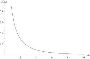
Figure 1: The graph of $\xi(a_{0})$ against $a_{0}$.

We note that the second derivative $\phi^{\prime\prime}(a_{0})>0$, and so the steepest descent direction is parallel to the imaginary axis. We find that

$$a_{N_{A},N_{c}} \sim \frac{1}{2\pi i}\int_{a_{0}-i\epsilon}^{a_{0}+i\epsilon}\mathrm{d}a~{}f(a_{0},N_{c})\exp\left(N_{c}\phi(a_{0})+\frac{1}{2}N_{c}\phi^{\prime\prime}(a_{0})(a-a_{0})^{2}\right)$$ (4.45)

$$= \frac{1}{2\pi}e^{N_{c}\phi(a_{0})}f(a_{0},N_{c})\int_{-\epsilon}^{\epsilon}\mathrm{d}\alpha~{}e^{-\frac{1}{2}N_{c}\phi^{\prime\prime}(a_{0})\alpha^{2}}\qquad\text{($a=a_{0}+i\alpha$)}$$

$$\sim \frac{1}{\pi}\frac{e^{N_{c}\phi(a_{0})}f(a_{0},N_{c})}{\sqrt{2N_{c}\phi^{\prime\prime}(a_{0})}}\int_{-\infty}^{\infty}\mathrm{d}s~{}e^{-s^{2}}\qquad\qquad\quad\;\text{$\left(s=\alpha\sqrt{\frac{1}{2}N_{c}\phi^{\prime\prime}(a_{0})}\right)$}$$

$$\sim \frac{e^{N_{c}\phi(a_{0})}f(a_{0},N_{c})}{\sqrt{2\pi N_{c}\phi^{\prime\prime}(a_{0})}}~{}.$$

Therefore, substituting (4.43) and (4.44) into (4.45), we have

$$a_{N_{A},N_{c}}=\frac{F(a_{0})}{N_{c}^{2}}\exp\left(N_{c}\left[\frac{2}{a_{0}}\left(\frac{\pi^{2}}{6}-\mathrm{Li}_{2}(e^{-a_{0}})\right)+\log\left(1-e^{-a_{0}}\right)\right]\right)~{},$$ (4.46)

where

$$F(a_{0}) = \frac{C(a_{0})}{\sqrt{2\pi\phi^{\prime\prime}(a_{0})}}\ ,$$

$$\phi^{\prime\prime}(a_{0}) = \frac{2}{a_{0}^{3}}\left(\frac{\pi^{2}}{6}-\mathrm{Li}_{2}(e^{-a_{0}})\right)+\frac{2}{a_{0}^{2}}\log(1-e^{-a_{0}})-\frac{1}{a_{0}(e^{a_{0}}-1)}\ .$$ (4.47)

Numerical values.

We compare numerical values of the logarithm of (4.46) with the logarithm of the corresponding exact value in Table 2.

$N_{c}$	$x$	Logarithm of (4.46)	Logarithm of the exact $a_{N_{A},N_{c}}$
50	1/2	74.640	75.333
100	1/2	157.58	158.28
50	1/4	53.180	53.945
100	1/4	114.06	114.84
100	1/8	80.008	80.837
1000	1/10	70.975	71.828

Table 2: Comparison of numerical values of the logarithm of (4.46) with the logarithm of the corresponding exact value.

4.3 The Canonical Free Energy

An immediate consequence of (3.1) is a general form of the unrefined generating function:

$$g^{(N_{f},SU(N_{c}))}(t)=\frac{P(t)}{\prod_{i}(1-t^{n_{i}})^{d_{i}}}~{},$$ (4.48)

where $P(t)$ is a palindromic polynomial with $P(1)\neq 0$, and the order of the pole $t=1$ of $g^{(N_{f},SU(N_{c}))}(t)$ is

$$\sum_{i}d_{i}=\dim{\cal M}_{(N_{f},SU(N_{c}))}=2N_{f}N_{c}~{}.$$ (4.49)

We can define the canonical free energy of the system as

$$F(t)=-\log g^{(N_{f},SU(N_{c}))}(t)~{}.$$ (4.50)

It is easy to see from (4.48), (4.49) and (4.50) that in the large and $N_{c}$ limit

$$F(t)\sim f(t)N_{f}N_{c}~{},$$ (4.51)

where $f(t)$ is some function of order 1. In other words, in this limit, the canonical free energy scales linearly with the dimension of the moduli space, which in turn is linear in both the number of colours and the number of flavours.

4.4 Complete Intersection Moduli Space

Having seen from a number of examples in preceding subsections that the moduli space of the theories with 1 flavour and 1 adjoint chiral multiplet is a complete intersection, we shall demonstrate that this statement is true for any $SU(N_{c})$ gauge group.

Generators and relations.

The generators of the theories with 1 flavour and 1 adjoint matter are

$$\begin{array}[]{llll}\mbox{\bf Casimir invariants}:&s^{k}&\rightarrow&u_{k}={\rm Tr}(\phi^{k}),~{}k=2,\ldots,\>N_{c}\\ &&&1~{}\text{operator for each $k$}~{},\\ \mbox{\bf Meson}:&t\tilde{t}&\rightarrow&M=Q_{a}\widetilde{Q}^{a}\\ &&&1~{}\text{operator}~{},\\ \mbox{\bf Adjoint mesons}:&s^{l}t\tilde{t}&\rightarrow&(A_{l})=Q_{a}\>(\phi^{l})^{a}_{b}\>\widetilde{Q}^{b},~{}l=1,\ldots,\>N_{c}-1\\ &&&1~{}\text{operator for each $l$}~{},\\ \mbox{\bf Adjoint baryon}:&s^{(N_{c}-1)N_{c}/2}t^{N_{c}}&\rightarrow&{\cal B}_{0,1,2,\ldots,N_{c}-1}=\epsilon^{abc\ldots d}Q_{a}{(P_{1})}_{b}{(P_{2})}_{c}\ldots(P_{N_{c}-1})_{d}\\ &&&\text{1 operator}~{},\\ \mbox{\bf Adjoint antibaryon}:&s^{(N_{c}-1)N_{c}/2}\tilde{t}^{N_{c}}&\rightarrow&\mbox{adjoint baryon with $Q\rightarrow\widetilde{Q}$}\\ &&&\text{1 operator}~{}.\\ \end{array}$$

We see that there are altogether $2N_{c}+1$ generators. Note that in all examples we checked the number of relations is 1. We therefore assume that there is precisely one basic relation at order $s^{(N_{c}-1)N_{c}}t^{N_{c}}\tilde{t}^{N_{c}}$.

Since the dimension of the moduli space (which is $2N_{c}$ from (3.1)) is equal to the number of generators (which is $2N_{c}+1$) minus the number of basic relations (which is assumed to be 1), it gives a strong indication that the moduli space is a complete intersection.

General formula.

As a consequence, we can write down a fully refined generating function for an arbitrary $N_{c}$ as

$$g^{(1,SU(N_{c}))}(s,t,\tilde{t})=\frac{1-s^{(N_{c}-1)N_{c}}t^{N_{c}}\tilde{t}^{N_{c}}}{(1-s^{(N_{c}-1)N_{c}/2}t^{N_{c}})(1-s^{(N_{c}-1)N_{c}/2}\tilde{t}^{N_{c}})\prod_{k=2}^{N_{c}}(1-s^{k})\prod_{l=0}^{N_{c}-1}(1-s^{l}t\tilde{t})}~{}.$$

4.4.1 A General Expression for The Relation

In §4.1.1, the relation for the case of $N_{c}=2,N_{f}=1$ is written explicitly in (4.9). It is interesting to find a general expression of the relation for any $N_{c}$ (with $N_{f}=1$). In this and only this subsection, we include the factor of $1/k$ into the Casimir invariant $u_{k}$, namely $u_{k}=\frac{1}{k}{\rm Tr}(\phi^{k})$.

The case of $N_{c}=3$.

Let us introduce the operators $A_{3}$ and $A_{4}$ in the usual way, i.e. $A_{l}=Q_{a}\>\phi^{l}\>\widetilde{Q}^{a}$. Note that they can be written in terms of basic generators as

$$A_{3}=u_{3}A_{0}+u_{2}A_{1}~{},\qquad A_{4}=u_{3}A_{1}+u_{2}A_{2}~{},$$ (4.53)

where $A_{0}$ denotes the meson $M$. Then, the relation can be written as

$${\cal B}\widetilde{{\cal B}}=A_{0}A_{2}A_{4}-A_{0}A_{3}^{2}+2A_{1}A_{2}A_{3}-A_{1}^{2}A_{4}-A_{2}^{3}~{},$$ (4.54)

where ${\cal B}$ and $\widetilde{{\cal B}}$ respectively denote the baryon and antibaryon. The moduli space is $\mathbb{C}^{9}/\mathcal{I}_{3}$, where the ideal $\mathcal{I}_{3}$ is given by the 3 relations: (4.53) and (4.54).

The case of $N_{c}=4$.

We introduce the operators $A_{4},\ldots,A_{6}$, which can be written in terms of basic generators as

$$A_{4} = u_{4}A_{0}-\frac{1}{2}u_{2}^{2}A_{0}+u_{3}A_{1}+u_{2}A_{2}~{},$$

$$A_{5} = u_{4}A_{1}-\frac{1}{2}u_{2}^{2}A_{1}+u_{3}A_{2}+u_{2}A_{3}~{},$$

$$A_{6} = u_{2}u_{4}A_{0}-\frac{1}{2}u_{2}^{3}A_{0}+u_{2}u_{3}A_{1}+\frac{1}{2}u_{2}^{2}A_{2}+u_{4}A_{2}+u_{3}A_{3}~{}.$$ (4.55)

Then, the relation can be written as

$${\cal B}\widetilde{{\cal B}} = A_{0}A_{2}A_{4}A_{6}-A_{0}A_{2}A_{5}^{2}-A_{0}A_{3}^{2}A_{6}+2A_{0}A_{3}A_{4}A_{5}-A_{0}A_{4}^{3}-A_{1}^{2}A_{4}A_{6}+A_{1}^{2}A_{5}^{2}$$ (4.56)

$$+2A_{1}A_{2}A_{3}A_{6}-2A_{1}A_{2}A_{4}A_{5}-2A_{1}A_{3}^{2}A_{5}+2A_{1}A_{3}A_{4}^{2}-A_{2}^{3}A_{6}+2A_{2}^{2}A_{3}A_{5}$$

$$+A_{2}^{2}A_{4}^{2}-3A_{2}A_{3}^{2}A_{4}+A_{3}^{4}~{}.$$

The moduli space is $\mathbb{C}^{12}/\mathcal{I}_{4}$, where the ideal $\mathcal{I}_{4}$ is given by the 4 relations: (4.55) and (4.56).

A general expression.

We can generalise (4.54) and (4.56) to any number of colours. The relation can be written compactly as

$${\cal B}\widetilde{{\cal B}} = \det\mathcal{A}~{},$$ (4.57)

where $\mathcal{A}_{ij}=A_{i+j}$ and $0\leq i,j\leq N_{c}-1$.

It is interesting to examine this formula in the spacial case of $N_{c}=2$. The adjoint baryon is given by ${\cal B}=\epsilon^{ab}Q^{1}_{a}(P_{1})^{1}_{b}=A^{11}$, whereas the adjoint antibaryon is given by $\widetilde{{\cal B}}=\epsilon_{ab}Q^{a2}(P_{1})^{b2}=\epsilon_{ab}\epsilon^{ad}Q_{d}^{2}\epsilon^{bc}(P_{1})_{c}^{2}=-\delta^{d}_{b}Q_{d}^{2}\epsilon^{bc}(P_{1})_{c}^{2}=-\epsilon^{bc}Q_{b}^{2}(P_{1})_{c}^{2}=-A^{22}~{}\text{(note the minus sign)}$. Similarly, it is easy to see that $\det\mathcal{A}=A_{0}A_{2}-A_{1}^{2}=M^{12}\left(\frac{1}{2}uM^{12}\right)-(A^{12})^{2}$. We thus correctly recover the formula (4.9).

The relations via Newton’s formula and the Cayley-Hamilton theorem.

Consider the characteristic polynomial $p(x)=\det(x\mathbb{I}-\phi)$ of $\phi$, which can be written as

$$p(x)=\sum_{j=0}^{N_{c}}x^{j}s_{N_{c}-j}~{},$$ (4.58)

with $s_{0}=1$ and $s_{1}=-{\rm Tr}(\phi)=0$. Note that $s_{k}$ is a symmetric polynomial $s_{k}=(-)^{k}\sum_{i_{1}<\ldots<i_{k}}\lambda_{i_{1}}\ldots\lambda_{i_{k}}$ and $u_{k}=\frac{1}{k}\sum_{i}\lambda_{i}^{k}$, where $\lambda$’s are the eigenvalues of $\phi$. It follows that the $u$’s and $s$’s are related by Newton’s formula (see e.g., [32, 33]):

$$ns_{n}+\sum_{j=1}^{n}ju_{j}s_{n-j}=0\qquad(2\leq n\leq N_{c})~{}.$$ (4.59)

Note that the case of $n=1$ is trivial. Using the Cayley–Hamilton theorem, one obtains the matrix relation:

$$p(\phi)=\sum_{j=0}^{N_{c}}\phi^{j}s_{N_{c}-j}=0~{}.$$ (4.60)

Multiplying (4.60) by $\phi^{m}$ (with $0\leq m\leq N_{c}-2$) and then by $Q$ to the left and $\widetilde{Q}$ to the right, one obtains

$$\sum_{j=0}^{N_{c}}A_{j+m}s_{N_{c}-j}=0\qquad(0\leq m\leq N_{c}-2)~{}.$$ (4.61)

Note that (4.59) gives $N_{c}-1$ relations between $u$’s and $s$’s and (4.61) gives $N_{c}-1$ relations between $A$’s and $s$’s.

Counting generators and relations.

There are altogether $4N_{c}-1$ variables: $A_{l}$ (with $l=0,\ldots,2N_{c}-2$); $s_{m}$, $u_{m}$ (with $m=2,\ldots,N_{c}$); ${\cal B}$, $\widetilde{{\cal B}}$. However, there are $2N_{c}-1$ relations: $N_{c}-1$ relations (4.59) between $u$’s and $s$’s; $N_{c}-1$ relations (4.61) between $A$’s and $s$’s; and 1 relation (4.57). Thus, by the assumption of the moduli space being a complete intersection, we find that the dimension of the moduli space is $2N_{c}$, in agreement with the earlier result.

5 The $Sp(N_{c})$ Gauge Groups

Let us turn to the $Sp(N_{c})$ gauge theory with $2N_{f}$ chiral superfields transforming in the fundamental representation ($N_{f}$ flavours) and 1 chiral superfield transforming in the adjoint representation. The anomaly-free global symmetry of this theory [24] is $SU(2N_{f})\times U(1)\times U(1)_{R}$.

5.1 Examples of Hilbert Series

Below we shall derive Hilbert series for various cases.

5.1.1 The $Sp(2)$ Gauge Group

Let us now examine the $Sp(2)$ gauge theory with $2N_{f}$ chiral multiplets in the fundamental representation and 1 chiral superfield in the adjoint representation. The Molien–Weyl formula for this theory is

$$g^{(N_{f},Sp(2))} = \int_{Sp(2)}d\mu_{Sp(2)}(z_{1},z_{2})PE\left[2N_{f}[1,0]t\;+[2,0]s\right]$$

$$= \oint\limits_{|z_{1}|=1}\frac{dz_{1}}{2\pi iz_{1}}\oint\limits_{|z_{2}|=1}\frac{dz_{2}}{2\pi iz_{2}}\frac{(1-z^{2}_{1})(1-z_{2})(1-\frac{z^{2}_{1}}{z_{2}})(1-\frac{z^{2}_{2}}{z^{2}_{1}})}{\left((1-tz_{1})(1-t\frac{z_{2}}{z_{1}})(1-t\frac{z_{1}}{z_{2}})(1-t\frac{1}{z_{1}})\right)^{2N_{f}}}\times$$

$$\frac{1}{(1-s)^{2}(1-sz^{2}_{1})(1-sz_{2})(1-s\frac{z^{2}_{1}}{z_{2}})(1-s\frac{z^{2}_{2}}{z^{2}_{1}})(1-s\frac{z^{2}_{1}}{z^{2}_{2}})(1-s\frac{z_{2}}{z^{2}_{1}})(1-s\frac{1}{z_{2}})(1-s\frac{1}{z^{2}_{1}})}$$

Applying the residue theorem, we can compute Hilbert series for various $N_{f}$:

$$g^{(1,Sp(2))}(s,t) = \frac{(1-s^{6}t^{4})(1-s^{4}t^{4})}{(1-s^{2})(1-s^{4})(1-t^{2})(1-st^{2})^{3}(1-s^{2}t^{2})(1-s^{3}t^{2})^{3}}~{},$$

$$= 1+s^{2}+2s^{4}+2s^{6}+3s^{8}+t^{2}+3st^{2}+2s^{2}t^{2}+6s^{3}t^{2}+3s^{4}t^{2}+9s^{5}t^{2}+4s^{6}t^{2}+$$

$$12s^{7}t^{2}+5s^{8}t^{2}+t^{4}+3st^{4}+8s^{2}t^{4}+9s^{3}t^{4}+18s^{4}t^{4}+15s^{5}t^{4}+30s^{6}t^{4}+$$

$$21s^{7}t^{4}+40s^{8}t^{4}+t^{6}+3st^{6}+8s^{2}t^{6}+19s^{3}t^{6}+24s^{4}t^{6}+43s^{5}t^{6}+45s^{6}t^{6}+$$

$$74s^{7}t^{6}+66s^{8}t^{6}+t^{8}+3st^{8}+8s^{2}t^{8}+19s^{3}t^{8}+39s^{4}t^{8}+53s^{5}t^{8}+90s^{6}t^{8}+$$

$$102s^{7}t^{8}+156s^{8}t^{8}+O(s^{9})O(t^{9})~{},$$

$$g^{(2,Sp(2))}(s,t) = 1+s^{2}+2s^{4}+2s^{6}+3s^{8}+6t^{2}+10st^{2}+12s^{2}t^{2}+20s^{3}t^{3}+18s^{4}t^{2}+30s^{5}t^{2}+$$

$$24s^{6}t^{2}+40s^{7}t^{2}+30s^{8}t^{2}+21t^{4}+60st^{4}+111s^{2}t^{4}+165s^{3}t^{4}+232s^{4}t^{4}+270s^{5}t^{4}+$$

$$357s^{6}t^{4}+375s^{7}t^{4}+478s^{8}t^{8}+56t^{6}+210st^{6}+500s^{2}t^{6}+890s^{3}t^{6}+1330s^{4}t^{6}+$$

$$1836s^{5}t^{6}+2300s^{6}t^{6}+2866s^{7}t^{6}+3270s^{8}t^{6}+126t^{8}+560st^{8}+1560s^{2}t^{8}+$$

$$3220s^{3}t^{8}+5405s^{4}t^{8}+7991s^{5}t^{8}+10955s^{6}t^{8}+13906s^{7}t^{8}+18190s^{8}t^{8}+O(s^{9})O(t^{9})~{},$$

$$g^{(3,Sp(2))}(s,t) = 1+s^{2}+2s^{4}+2s^{6}+3s^{8}+15t^{2}+21st^{2}+30s^{2}t^{2}+42s^{3}t^{2}+45s^{4}t^{2}+63s^{5}t^{2}+$$

$$60s^{6}t^{2}+84s^{7}t^{2}+75s^{8}t^{2}+120t^{4}+315st^{4}+561s^{2}t^{4}+840s^{3}t^{4}+1122s^{4}t^{4}+$$

$$1365s^{5}t^{4}+1689s^{6}t^{4}+1890s^{7}t^{4}+2250s^{8}t^{4}+679t^{6}+2485st^{6}+5530s^{2}t^{6}+$$

$$9436s^{3}t^{6}+13895s^{4}t^{6}+18571s^{5}t^{6}+23310s^{6}t^{6}+28168s^{7}t^{6}+32725s^{8}t^{6}+$$

$$3045t^{8}+13770st^{8}+36120s^{2}t^{8}+70050s^{3}t^{8}+113190s^{4}t^{8}+162960s^{5}t^{8}+$$

$$216825s^{6}t^{8}+272160s^{7}t^{8}+328896s^{8}t^{8}+O(s^{9})O(t^{9})~{},$$

$$g^{(4,Sp(2))}(s,t) = 1+s^{2}+2s^{4}+2s^{6}+3s^{8}+28t^{2}+36st^{2}+56s^{2}t^{2}+72s^{3}t^{2}+84s^{4}t^{2}+108s^{5}t^{2}+$$ (5.63)

$$112s^{6}t^{2}+144s^{7}t^{2}+140s^{8}t^{2}+406t^{4}+1008st^{4}+1786s^{2}t^{4}+2646s^{3}t^{4}+3488s^{4}t^{4}+$$

$$4284s^{5}t^{4}+5198s^{6}t^{4}+5922s^{7}t^{4}+6900s^{8}t^{4}+4032t^{6}+14196st^{6}+30576s^{2}t^{6}+$$

$$51192s^{3}t^{6}+74424s^{4}t^{6}+98352s^{5}t^{6}+122892s^{6}t^{6}+147228s^{7}t^{6}+171360s^{8}t^{6}+$$

$$30744t^{8}+135120st^{8}+340641s^{2}t^{8}+640800s^{3}t^{8}+1015092s^{4}t^{8}+1438332s^{5}t^{8}+$$

$$1889421s^{6}t^{8}+2351496s^{7}t^{8}+2819127s^{8}t^{8}+O(s^{9})(t^{9})~{}.$$

A general form of the generating function when we set $s=t=\tilde{t}$ is

$$g^{(N_{f},Sp(2))}(t) = \frac{P_{24N_{f}-16}(t)}{(1+t)^{6N_{f}-7}(1-t^{2})^{2N_{f}+1}(1+t^{2})(1-t^{3})^{4N_{f}-1}(1-t^{5})^{2N_{f}}}~{}.$$ (5.64)

Plethystic Logarithms.

We shall calculate the plethystic logarithms of the generating functions using formula (2.16):

$$\mathrm{PL}\left[g^{(1,Sp(2))}(s,t)\right] = s^{2}+s^{4}+t^{2}+3st^{2}+s^{2}t^{2}+3s^{3}t^{2}-s^{4}t^{4}-s^{6}t^{4}~{},$$

$$\mathrm{PL}\left[g^{(2,Sp(2))}(s,t)\right] = s^{2}+s^{4}+6t^{2}+10st^{2}+6s^{2}t^{2}+10s^{3}t^{2}-s^{2}t^{4}-15s^{3}t^{4}-21s^{4}t^{4}-15s^{5}t^{4}$$

$$-20s^{6}t^{4}-6s^{2}t^{6}-10s^{3}t^{6}+16s^{5}t^{6}+86s^{6}t^{6}+90s^{7}t^{6}+80s^{8}t^{6}+15s^{3}t^{8}$$

$$+51s^{4}t^{8}+140s^{5}t^{8}+120s^{6}t^{8}-31s^{7}t^{8}-236s^{8}t^{8}+O(s^{9})O(t^{9})~{},$$

$$\mathrm{PL}\left[g^{(3,Sp(2))}(s,t)\right] = s^{2}+s^{4}+15t^{2}+21st^{2}+15s^{2}t^{2}+21s^{3}t^{2}-15s^{2}t^{4}-105s^{3}t^{4}-120s^{4}t^{4}$$

$$-105s^{5}t^{4}-105s^{6}t^{4}-t^{6}-35st^{6}-189s^{2}t^{6}-175s^{3}t^{6}+36s^{4}t^{6}+539s^{5}t^{6}$$

$$+1589s^{6}t^{6}+1575s^{7}t^{6}+1365s^{8}t^{6}+36st^{8}+540s^{2}t^{8}+2100s^{3}t^{8}+5019s^{4}t^{8}$$

$$+8118s^{5}t^{8}+4185s^{6}t^{8}-4515s^{7}t^{8}-16869s^{8}t^{8}+O(s^{9})O(t^{9})~{},$$

$$\mathrm{PL}\left[g^{(4,Sp(2))}(s,t)\right] = s^{2}+s^{4}+28t^{2}+36st^{2}+28s^{2}t^{2}+36s^{3}t^{2}-70s^{2}t^{4}-378s^{3}t^{4}-406s^{4}t^{4}$$ (5.65)

$$-378s^{5}t^{4}-336s^{6}t^{4}-28t^{6}-420st^{6}-1512s^{2}t^{6}-1176s^{3}t^{6}+448s^{4}t^{6}$$

$$+4452s^{5}t^{6}+10920s^{6}t^{6}+10584s^{7}t^{6}+8988s^{8}t^{6}+63t^{8}+1728st^{8}$$

$$+12481s^{2}t^{8}+38220s^{3}t^{8}+80493s^{4}t^{8}+108432s^{5}t^{8}+41615s^{6}t^{8}$$

$$-81564s^{7}t^{8}-247521s^{8}t^{8}+O(s^{9})O(t^{9})~{}.$$

5.1.2 The $Sp(3)$ Gauge Group

We now move to examining the generating funtions and their plethystic logarithms for the $Sp(3)$ gauge group with $2N_{f}$ chiral fields transforming in the fundamental representation and one in the adjoint representation of the group. The Molien-Weyl formula for this theory is

$$g^{(N_{f},Sp(3))} = \int_{Sp(3)}d\mu_{Sp(3)}(z_{1},z_{2},z_{3})\mathrm{PE}\left[2N_{f}[1,0,0]t\;+[2,0,0]s\right]$$

$$= \oint\limits_{|z_{1}|=1}\frac{dz_{1}}{2\pi iz_{1}}\oint\limits_{|z_{2}|=1}\frac{dz_{2}}{2\pi iz_{2}}\oint\limits_{|z_{3}|=1}\frac{dz_{3}}{2\pi iz_{3}}\frac{(1-z^{2}_{1})(1-\frac{z^{2}_{1}}{z_{2}})(1-z_{2})(1-\frac{z^{2}_{2}}{z^{2}_{1}})(1-\frac{z_{1}z_{2}}{z_{3}})}{(1-s\frac{1}{z^{2}_{1}})(1-sz^{2}_{1})(1-s\frac{z^{2}_{1}}{z^{2}_{2}})(1-s\frac{1}{z_{2}})(1-s\frac{z^{2}_{1}}{z_{2}})}\times$$

$$\frac{(1-\frac{z^{2}_{2}}{z_{1}z_{3}})(1-\frac{z_{3}}{z_{1}})(1-\frac{z_{1}z_{3}}{z_{2}})(1-\frac{z^{2}_{3}}{z^{2}_{2}})}{(1-s\frac{z^{2}_{2}}{z^{2}_{1}})(1-s\frac{z^{2}_{2}}{z^{2}_{3}})(1-s\frac{z_{1}}{z_{3}})(1-s\frac{z_{2}}{z_{1}z_{3}})(1-s\frac{z_{1}z_{2}}{z_{3}})(1-s\frac{z^{2}}{z_{1}z_{3}})(1-s\frac{z_{3}}{z_{1}})(1-s\frac{z_{1}z_{3}}{z^{2}_{2}})}\times$$

$$\frac{1}{(1-s\frac{z_{3}}{z_{1}z_{2}})(1-s\frac{z_{2}}{z^{2}_{1}})(1-s\frac{z_{1}z_{3}}{z_{2}})(1-s\frac{z^{2}_{3}}{z^{2}_{2}})(1-sz_{2})(1-s)^{3}((1-t\frac{1}{z_{1}})(1-tz_{1}))^{2N_{f}}}\times$$

$$\frac{1}{((1-t\frac{z_{1}}{z_{2}})(1-t\frac{z_{2}}{z_{1}})(1-t\frac{z_{2}}{z_{3}})(1-t\frac{z_{3}}{z_{2}}))^{2N_{f}}}$$

Applying the residue theorem we can compute Hilbert series for various $N_{f}$:

$$g^{(1,Sp(3))}(s,t) = \frac{(1-s^{6}t^{4})(1-s^{8}t^{4})(1-s^{10}t^{4})}{(1-s^{2})(1-s^{4})(1-s^{6})(1-t^{2})(1-st^{2})^{3}(1-s^{2}t^{2})(1-s^{3}t^{2})^{3}(1-s^{4}t^{2})(1-s^{5}t^{2})^{3}}~{},$$

$$= 1+s^{2}+2s^{4}+3s^{6}+4s^{8}+t^{2}+3st^{2}+2s^{2}t^{2}+6s^{3}t^{2}+4s^{4}t^{2}+12s^{5}t^{2}+6s^{6}t^{2}+$$

$$18s^{7}t^{2}+9s^{8}t^{2}+t^{4}+3st^{4}+8s^{2}t^{4}+9s^{3}t^{4}+20s^{4}t^{4}+21s^{5}t^{4}+43s^{6}t^{4}+$$

$$36s^{7}t^{4}+71s^{8}t^{4}+t^{6}+3st^{6}+8s^{2}t^{6}+19s^{3}t^{6}+26s^{4}t^{6}+52s^{5}t^{6}+65s^{6}t^{6}+$$

$$116s^{7}t^{6}+123s^{8}t^{6}+t^{8}+3st^{8}+8s^{2}t^{8}+19s^{3}t^{8}+41s^{4}t^{8}+62s^{5}t^{8}+116s^{6}t^{8}+$$

$$157s^{7}t^{8}+265s^{8}t^{8}+O(s^{9})O(t^{9})~{},$$

$$g^{(2,Sp(3))}(s,t) = 1+s^{2}+2s^{4}+3s^{6}+4s^{8}+6t^{2}+10st^{2}+12s^{2}t^{2}+20s^{3}t^{2}+24s^{4}t^{2}+40s^{5}t^{2}+$$

$$36s^{6}t^{2}+60s^{7}t^{2}+54s^{8}t^{2}+21t^{4}+60st^{4}+112s^{2}t^{4}+180s^{3}t^{4}+289s^{4}t^{4}+405s^{5}t^{4}+$$

$$571s^{6}t^{4}+690s^{7}t^{4}+939s^{8}t^{4}+56t^{6}+210st^{6}+512s^{2}t^{6}+1000s^{3}t^{6}+1738s^{4}t^{6}+$$

$$2790s^{5}t^{6}+4094s^{6}t^{6}+5770s^{7}t^{6}+7600s^{8}t^{6}+126t^{8}+560st^{8}+1617s^{2}t^{8}+3700s^{3}t^{8}+$$

$$7257s^{4}t^{8}+12725s^{5}t^{8}+20552s^{6}t^{8}+30860s^{7}t^{8}+44162s^{8}t^{8}+O(s^{9})O(t^{9})~{},$$

$$g^{(3,Sp(3))}(s,t) = 1+s^{2}+2s^{4}+3s^{6}+4s^{8}+15t^{2}+21st^{2}+30s^{2}t^{2}+42s^{3}t^{2}+60s^{4}t^{2}+84s^{5}t^{2}+$$

$$90s^{6}t^{2}+126s^{7}t^{2}+135s^{8}t^{2}+120t^{4}+315st^{4}+576s^{2}t^{4}+945s^{3}t^{4}+1467s^{4}t^{4}+$$

$$2100s^{5}t^{4}+2820s^{6}t^{4}+3570s^{7}t^{4}+4608s^{8}t^{4}+680t^{6}+2520st^{6}+5944s^{2}t^{6}+11501s^{3}t^{6}+$$

$$19889s^{4}t^{6}+31262s^{5}t^{6}+45629s^{6}t^{6}+63000s^{7}t^{6}+83549s^{8}t^{6}+3060t^{8}+14280st^{8}+$$

$$40950s^{2}t^{8}+92274s^{3}t^{8}+178626s^{4}t^{8}+308589s^{5}t^{8}+488922s^{6}t^{8}+724509s^{7}t^{8}+$$

$$1019424s^{8}t^{8}+O(s^{9})O(t^{9})~{},$$

$$g^{(4,Sp(3))}(s,t) = 1+s^{2}+2s^{4}+3s^{6}+4s^{8}+28t^{2}+36st^{2}+56s^{2}t^{2}+72s^{3}t^{2}+112s^{4}t^{2}+144s^{5}t^{2}+$$ (5.2)

$$168s^{6}t^{2}+216s^{7}t^{2}+252s^{8}t^{2}+406t^{4}+1008st^{4}+1856s^{2}t^{4}+3024s^{3}t^{4}+4678s^{4}t^{4}+$$

$$6678s^{5}t^{4}+8874s^{6}t^{4}+11340s^{7}t^{4}+14442s^{8}t^{4}+4060t^{6}+14616st^{6}+34048s^{2}t^{6}+$$

$$65472s^{3}t^{6}+112280s^{4}t^{6}+175044s^{5}t^{6}+253764s^{6}t^{6}+348276s^{7}t^{6}+460768s^{8}t^{6}+$$

$$31464t^{8}+146097st^{8}+414036s^{2}t^{8}+922593s^{3}t^{8}+1765443s^{4}t^{8}+3014997s^{5}t^{8}+$$

$$4727424s^{6}t^{8}+6942129s^{7}t^{8}+9691512s^{8}t^{8}+O(s^{9})(t^{9})~{}.$$

Plethystic Logarithms.

We shall calculate the plethystic logarithms of the generating functions using formula (2.16):

$$\mathrm{PL}\left[g^{(1,Sp(3))}(s,t)\right] = s^{2}+s^{4}+s^{6}+t^{2}+3st^{2}+s^{2}t^{2}+3s^{3}t^{2}+s^{4}t^{2}+3s^{5}t^{2}-s^{6}t^{4}-s^{8}t^{4}-s^{10}t^{4}~{},$$

$$\mathrm{PL}\left[g^{(2,Sp(3))}(s,t)\right] = s^{2}+s^{4}+s^{6}+6t^{2}+10st^{2}+6s^{2}t^{2}+10s^{3}t^{2}+6s^{4}t^{2}+10s^{5}t^{2}-s^{4}t^{4}-15s^{5}t^{4}-$$

$$21s^{6}t^{4}-15s^{7}t^{4}-21s^{8}t^{4}-6s^{4}t^{6}-10s^{5}t^{6}-6s^{6}t^{6}-10s^{7}t^{6}-s^{4}t^{8}+15s^{7}t^{8}+$$

$$52s^{8}t^{8}+O(s^{9})O(t^{9})~{},$$

$$\mathrm{PL}\left[g^{(3,Sp(3))}(s,t)\right] = s^{2}+s^{4}+s^{6}+15t^{2}+21st^{2}+15s^{2}t^{2}+21s^{3}t^{2}+15s^{4}t^{2}+21s^{5}t^{2}-15s^{4}t^{4}-$$

$$105s^{5}t^{4}-120s^{6}t^{4}-105s^{7}t^{4}-120s^{8}t^{4}-s^{2}t^{6}-35s^{3}t^{6}-190s^{4}t^{6}-210s^{5}t^{6}-$$

$$189s^{6}t^{6}-175s^{7}t^{6}+36s^{8}t^{6}-15s^{2}t^{8}-105s^{3}t^{8}-105s^{4}t^{8}+36s^{5}t^{8}+555s^{6}t^{8}+$$

$$2241s^{7}t^{8}+5679s^{8}t^{8}+O(s^{9})O(t^{9})~{},$$

$$\mathrm{PL}\left[g^{(4,Sp(3))}(s,t)\right] = s^{2}+s^{4}+s^{6}+28t^{2}+36st^{2}+28s^{2}t^{2}+36s^{3}t^{2}+28s^{4}t^{2}+36s^{5}t^{2}-70s^{4}t^{4}-$$ (5.3)

$$378s^{5}t^{4}-406s^{6}t^{4}-378s^{7}t^{4}-406s^{8}t^{4}-28s^{2}t^{6}-420s^{3}t^{6}-1540s^{4}t^{6}-1596s^{5}t^{6}-$$

$$1512s^{6}t^{6}-1176s^{7}t^{6}+448s^{8}t^{6}-t^{8}-63st^{8}-720s^{2}t^{8}-2352s^{3}t^{8}-1700s^{4}t^{8}+$$

$$1791s^{5}t^{8}+13265s^{6}t^{8}+42363s^{7}t^{8}+95521s^{8}t^{8}+O(s^{9})O(t^{9})~{}.$$

5.2 Generators of the Chiral Ring

Below we summarise the generators of $Sp(N_{c})$ adjoint SQCD [23, 24] and representations of $SU(2N_{f})\times SU(2N_{f})$ in which they transform.

$$\begin{array}[]{llllll}\mbox{\bf Casimir invariants}:&s^{2k}&\rightarrow&u_{2k}={\rm Tr}(\phi^{2k})\qquad(k=1,\>2,\>\ldots,N_{c})\\ &&&[0,\ldots,0]\quad 1~{}\text{dimensional}~{},\\ \mbox{\bf Mesons}:&t^{2}&\rightarrow&M^{ij}=J^{ab}Q^{i}_{a}{Q}^{j}_{b}\qquad(a,b=1,\>2,\>\ldots,2N_{c})\\ &&&[0,1,0,\ldots,0]\quad N_{f}(2N_{f}-1)~{}\text{dimensional}~{},\\ \mbox{\bf Even adjoint mesons}:&s^{2l}t^{2}&\rightarrow&(A_{2l})^{ij}=J^{a_{1}b_{1}}J^{c_{1}b_{2}}J^{c_{2}b_{3}}\ldots J^{c_{2l-1}b_{2l}}J^{c_{2l}a_{2l}}Q^{i}_{a_{1}}\phi_{b_{1}c_{1}}\phi_{b_{2}c_{2}}\ldots\phi_{b_{2l}c_{2l}}Q^{j}_{a_{2l}}\\ &&&[0,1,0,\ldots,0]\quad N_{f}(2N_{f}-1)~{}\text{dimensional}\quad(l=1,\ldots,N_{c}-1)~{},\\ \mbox{\bf Odd adjoint mesons}:&s^{2k-1}t^{2}&\rightarrow&(A_{2k-1})^{ij}=J^{a_{1}b_{1}}J^{c_{1}b_{2}}\ldots J^{c_{2k-1}a_{2k-1}}Q^{i}_{a_{1}}\phi_{b_{1}c_{1}}\phi_{b_{2}c_{2}}\ldots\phi_{b_{2k-1}c_{2k-1}}Q^{j}_{a_{2k-1}}\\ &&&[2,0,\ldots,0]\quad N_{f}(2N_{f}+1)~{}\text{dimensional}\quad(k=1,\ldots,N_{c})~{},\\ \end{array}$$

The total number of generators is

$$N_{c}(1+4N_{f}^{2})~{}.$$ (5.4)

We note that for $N_{c}=1$, $Sp(1)$ is isomorphic to $SU(2)$. In which case, we recover the $SU(2)$ adjoint SQCD and hence (5.4) reduces to (4.7).

5.3 Complete Intersection Moduli Space

We claim that the moduli space of the $Sp(N_{c})$ adjoint SQCD with $2$ fundamental chiral multiplets ($N_{f}=1$) and 1 adjoint chiral multiplet is a complete intersection. A general expression of the phethystic logarithm for the complete intersection case can be written as

$$\mathrm{PL}[g^{(1,Sp(N_{c}))}(s,t)]=\sum^{N_{c}}_{k=1}s^{2k}+\sum^{N_{c}}_{k=1}(3s^{2k-1}+s^{2(k-1)})t^{2}-\sum^{N_{c}}_{k=1}s^{2(N_{c}+k-1)}t^{4}~{}.$$ (5.5)

Note that the number of relations is equal to the rank of the gauge group and not to 1 as might naively be expected from the case of $SU(N_{c})$ gauge group.

6 The $SO(N_{c})$ Gauge Groups

Let us turn to the $SO(N_{c})$ gauge theory with $N_{f}$ chiral superfields transforming in the fundamental (vector) representation ($N_{f}$ flavours) and 1 chiral superfield transforming in the adjoint representation. The global symmetry of this theory [23] is $SU(N_{f})\times U(1)_{R}$.

6.1 Examples of Hilbert Series

We shall derive Hilbert series for various cases. Note that the following subsections are not merely a collection of results. They will turn out to be essential for analysing the generators of the chiral ring.

6.1.1 The $SO(3)$ Gauge Group

Let us now examine the $SO(3)$ gauge theory with $N_{f}$ chiral multiplets in the fundamental representation and 1 chiral superfield in the adjoint representation. The Molien–Weyl formula for this theory is

$$g^{(N_{f},SO(3))} = \frac{1}{2\pi i}\oint_{|z|=1}\frac{dz}{z}(1-z)~{}\mathrm{PE}\>\left[N_{f}[1]t+[1]s\right]$$ (6.1)

$$= \frac{1}{2\pi i}\oint_{|z|=1}\frac{dz}{z}\frac{1-z}{(1-t)^{N_{f}}(1-tz)^{N_{f}}(1-\frac{t}{z})^{N_{f}}(1-s)(1-sz)(1-\frac{s}{z})}~{}.\quad$$

Applying the residue theorem, we find that

$$g^{(1,SO(3))}(s,t) = \frac{1}{\left(1-s^{2}\right)(1-st)\left(1-t^{2}\right)}~{},$$

$$g^{(2,SO(3))}(s,t) = \frac{1-s^{2}t^{4}}{\left(1-s^{2}\right)(1-st)^{2}(1-st^{2})\left(1-t^{2}\right)^{3}}~{},$$

$$g^{(3,SO(3))}(s,t) = \frac{1-t+t^{2}+3st^{2}-3st^{3}-s^{2}t^{3}+s^{2}t^{4}-s^{2}t^{5}}{(1-s^{2})(1-t)^{6}(1+t)^{5}(1-st)^{3}}~{},$$

$$g^{(4,SO(3))}(s,t) = 1+s^{2}+s^{4}+4st+4s^{3}t+10t^{2}+6st^{2}+20s^{2}t^{2}+6s^{3}t^{2}+20s^{4}t^{2}+4t^{3}$$ (6.2)

$$+40st^{3}+24s^{2}t^{3}+60s^{3}t^{3}+24s^{4}t^{3}+55t^{4}+60st^{4}+155s^{2}t^{4}+105s^{3}t^{4}$$

$$+190s^{4}t^{4}+O(s^{5})O(t^{5})~{}.$$

Plethystic logarithms.

We shall calculate plethystic logarithms of generating functions using formula (2.16):

$$\mathrm{PL}\left[g^{(1,SO(3))}(s,t)\right] = s^{2}+st+t^{2}~{},$$

$$\mathrm{PL}\left[g^{(2,SO(3))}(s,t)\right] = s^{2}+2st+3t^{2}+st^{2}-s^{2}t^{4}~{},$$

$$\mathrm{PL}\left[g^{(3,SO(3))}(s,t)\right] = s^{2}+3st+6t^{2}+3st^{2}+t^{3}-s^{2}t^{3}-3st^{4}-6s^{2}t^{4}+O(s^{5})O(t^{5})~{},$$

$$\mathrm{PL}\left[g^{(4,SO(3))}(s,t)\right] = s^{2}+4st+10t^{2}+6st^{2}+4t^{3}-4s^{2}t^{3}-16st^{4}-21s^{2}t^{4}+s^{3}t^{4}+O(s^{5})O(t^{5})~{}.\qquad\quad$$ (6.3)

The $N_{f}=1$ moduli space is freely generated, i.e. there is no relation between the generators. Since the plethystic logarithm for $N_{f}=2$ is a polynomial (not an infinite series), it follows that the $N_{f}=2$ moduli space is a complete intersection.

6.1.2 The $SO(4)$ Gauge Group

Let us now examine the $SO(4)$ gauge theory with $N_{f}$ chiral multiplets in the fundamental representation and 1 chiral superfield in the adjoint representation. The Molien–Weyl formula for this theory is

$$g^{(N_{f},SO(4))} = \frac{1}{(2\pi i)^{2}}\oint_{|z_{1}|=1}\frac{dz_{1}}{z_{1}}\oint_{|z_{2}|=1}\frac{dz_{2}}{z_{2}}\left(1-\frac{z_{1}}{z_{2}}\right)(1-z_{1}z_{2})$$ (6.4)

$$\times\mathrm{PE}\>\left[N_{f}[1,0]t+[1,1]s\right]~{}.\qquad$$

Applying the residue theorem, we find that

$$g^{(1,SO(4))}(s,t) = \frac{1}{\left(1-s^{2}\right)^{2}\left(1-t^{2}\right)\left(1-s^{2}t^{2}\right)}~{},$$

$$g^{(2,SO(4))}(s,t) = \frac{(1-s^{2}t^{4})(1-s^{4}t^{4})}{(1-s^{2})^{2}(1-t^{2})^{3}(1-st^{2})^{2}(1-s^{2}t^{2})^{3}}~{},$$

$$g^{(3,SO(4))}(s,t) = \frac{1+3st^{2}+3s^{2}t^{2}+3s^{3}t^{4}-2s^{2}t^{6}-8s^{3}t^{6}-8s^{4}t^{6}-2s^{5}t^{6}+3s^{4}t^{8}+3s^{5}t^{10}+3s^{6}t^{10}+s^{7}t^{12}}{\left(1-s^{2}\right)^{2}(1-st)^{3}(1+st)^{3}\left(1-t^{2}\right)^{6}\left(1-st^{2}\right)^{3}}~{},$$

$$g^{(4,SO(4))}(s,t) = 1+2s^{2}+3s^{4}+10t^{2}+12st^{2}+30s^{2}t^{2}+24s^{3}t^{2}+50s^{4}t^{2}+56t^{4}+120st^{4}+267s^{2}t^{4}+$$

$$330s^{3}t^{4}+513s^{4}t^{4}+O(s^{5})O(t^{5})~{},$$

$$g^{(5,SO(4))}(s,t) = 1+2s^{2}+3s^{4}+15t^{2}+20st^{2}+45s^{2}t^{2}+40s^{3}t^{2}+75s^{4}t^{2}+125t^{4}+300st^{4}+620s^{2}t^{4}+$$ (6.5)

$$810s^{3}t^{4}+1185s^{4}t^{4}+O(s^{5})O(t^{5})~{}.$$

Plethystic logarithms.

We shall calculate plethystic logarithms of generating functions using formula (2.16):

$$\mathrm{PL}\left[g^{(1,SO(4))}(s,t)\right] = 2s^{2}+t^{2}+s^{2}t^{2}~{},$$

$$\mathrm{PL}\left[g^{(2,SO(4))}(s,t)\right] = 2s^{2}+3t^{2}+2st^{2}+3s^{2}t^{2}-s^{2}t^{4}-s^{4}t^{4}~{},$$

$$\mathrm{PL}\left[g^{(3,SO(4))}(s,t)\right] = 2s^{2}+6t^{2}+6st^{2}+6s^{2}t^{2}-6s^{2}t^{4}-6s^{3}t^{4}-6s^{4}t^{4}+O(s^{5})O(t^{5})~{},$$

$$\mathrm{PL}\left[g^{(4,SO(4))}(s,t)\right] = 2s^{2}+10t^{2}+12st^{2}+10s^{2}t^{2}+t^{4}-23s^{2}t^{4}-30s^{3}t^{4}-20s^{4}t^{4}+O(s^{5})O(t^{5})~{},$$

$$\mathrm{PL}\left[g^{(5,SO(4))}(s,t)\right] = 2s^{2}+15t^{2}+20st^{2}+15s^{2}t^{2}+5t^{4}-65s^{2}t^{4}-90s^{3}t^{4}-50s^{4}t^{4}+O(s^{5})O(t^{5})~{},$$

$$\mathrm{PL}\left[g^{(6,SO(4))}(s,t)\right] = 2s^{2}+21t^{2}+30st^{2}+21s^{2}t^{2}+15t^{4}-150s^{2}t^{4}-210s^{3}t^{4}-105s^{4}t^{4}+O(s^{5})O(t^{5})~{}.$$

The $N_{f}=1$ moduli space is freely generated, i.e. there is no relation between the generators. Since the plethystic logarithm for $N_{f}=2$ is a polynomial (not an infinite series), it follows that the $N_{f}=2$ moduli space is a complete intersection.

6.1.3 The $SO(5)$ Gauge Group

Let us now examine the $SO(5)$ gauge theory with $N_{f}$ chiral multiplets in the fundamental representation $[1,0]$ and 1 chiral superfield in the adjoint representation $[0,2]$. The Molien–Weyl formula for this theory is

$$g^{(N_{f},SO(5))} = \frac{1}{(2\pi i)^{2}}\oint_{|z_{1}|=1}\frac{dz_{1}}{z_{1}}\oint_{|z_{2}|=1}\frac{dz_{2}}{z_{2}}\left(1-z_{1}\right)\left(1-\frac{z_{1}^{2}}{z_{2}^{2}}\right)\left(1-z_{2}^{2}\right)\left(1-\frac{z_{2}^{2}}{z_{1}}\right)$$ (6.7)

$$\times\mathrm{PE}\>\left[N_{f}[1,0]t+[0,2]s\right]~{}.$$

Applying the residue theorem, we find that

$$g^{(1,SO(5))}(s,t) = \frac{1}{(1-s^{2})(1-s^{4})(1-s^{2}t)(1-t^{2})(1-s^{2}t^{2})}~{},$$

$$g^{(2,SO(5))}(s,t) = \frac{(1-s^{4}t^{4})(1-s^{6}t^{4})}{(1-s^{2})(1-s^{4})(1-s^{2}t)^{2}(1-t^{2})^{3}(1-st^{2})(1-s^{2}t^{2})^{3}(1-s^{3}t^{2})}~{},$$

$$g^{(3,SO(5))}(s,t) = \frac{1}{(1-s)^{2}(1+s)^{2}(1+s^{2})(1-t)^{6}(1+t)^{6}(1-st)^{3}(1+st)^{3}(1-s^{2}t)^{3}(1-st^{2})^{3}}\times$$

$$(1+3s^{2}t^{2}+3s^{3}t^{2}+st^{3}-s^{5}t^{3}-3s^{3}t^{4}+6s^{5}t^{4}+3s^{3}t^{5}-3s^{7}t^{5}-s^{4}t^{6}-9s^{5}t^{6}-9s^{6}t^{6}$$

$$-s^{7}t^{6}-3s^{4}t^{7}+3s^{8}t^{7}+6s^{6}t^{8}-3s^{8}t^{8}-s^{6}t^{9}+s^{10}t^{9}+3s^{8}t^{10}+3s^{9}t^{10}+s^{11}t^{12})~{}.$$

Plethystic logarithms.

We shall calculate plethystic logarithms of generating functions using formula (2.16):

$$\mathrm{PL}\left[g^{(1,SO(5))}(s,t)\right] = s^{2}+s^{4}+s^{2}t+t^{2}+s^{2}t^{2}~{},$$

$$\mathrm{PL}\left[g^{(2,SO(5))}(s,t)\right] = s^{2}+s^{4}+2s^{2}t+3t^{2}+st^{2}+3s^{2}t^{2}+s^{3}t^{2}-s^{4}t^{4}-s^{6}t^{4}~{},$$

$$\mathrm{PL}\left[g^{(3,SO(5))}(s,t)\right] = s^{2}+s^{4}+3s^{2}t+6t^{2}+3st^{2}+6s^{2}t^{2}+3s^{3}t^{2}+st^{3}-s^{5}t^{3}-3s^{3}t^{4}$$

$$-6s^{4}t^{4}-3s^{5}t^{4}-6s^{6}t^{4}-3s^{4}t^{5}-s^{2}t^{6}-s^{4}t^{6}+9s^{6}t^{6}+O(s^{7})O(t^{7})~{},$$

$$\mathrm{PL}\left[g^{(4,SO(5))}(s,t)\right] = s^{2}+s^{4}+4s^{2}t+10t^{2}+6st^{2}+10s^{2}t^{2}+6s^{3}t^{2}+4st^{3}-4s^{5}t^{3}-16s^{3}t^{4}$$

$$-21s^{4}t^{4}-15s^{5}t^{4}-21s^{6}t^{4}-4s^{3}t^{5}-24s^{4}t^{5}-10s^{2}t^{6}-6s^{3}t^{6}-10s^{4}t^{6}$$

$$+10s^{5}t^{6}+102s^{6}t^{6}+O(s^{7})O(t^{7})~{},$$

$$\mathrm{PL}\left[g^{(5,SO(5))}(s,t)\right] = s^{2}+s^{4}+5s^{2}t+15t^{2}+10st^{2}+15s^{2}t^{2}+10s^{3}t^{2}+10st^{3}-10s^{5}t^{3}$$

$$-50s^{3}t^{4}-55s^{4}t^{4}-45s^{5}t^{4}-55s^{6}t^{4}+t^{5}-s^{2}t^{5}-24s^{3}t^{5}-101s^{4}t^{5}+s^{5}t^{5}$$

$$+s^{6}t^{5}-60s^{2}t^{6}-45s^{3}t^{6}-50s^{4}t^{6}+75s^{5}t^{6}+555s^{6}t^{6}+O(s^{7})O(t^{7})~{}.$$

The $N_{f}=1$ moduli space is freely generated, i.e. there is no relation between the generators. Since the plethystic logarithm for $N_{f}=2$ is a polynomial (not an infinite series), it follows that the $N_{f}=2$ moduli space is a complete intersection.

6.1.4 The $SO(6)$ Gauge Group

Let us now examine the $SO(6)$ gauge theory with $N_{f}$ chiral multiplets in the fundamental representation and 1 chiral superfield in the adjoint representation. The Molien–Weyl formula for this theory is

$$g^{(N_{f},SO(6))} = \frac{1}{(2\pi i)^{3}}\oint_{|z_{1}|=1}\frac{dz_{1}}{z_{1}}\oint_{|z_{2}|=1}\frac{dz_{2}}{z_{2}}\oint_{|z_{3}|=1}\frac{dz_{3}}{z_{3}}\left(1-\frac{z_{2}^{2}}{z_{1}}\right)\left(1-\frac{z_{1}^{2}}{z_{2}z_{3}}\right)\left(1-\frac{z_{1}z_{2}}{z_{3}}\right)\times$$ (6.10)

$$\left(1-\frac{z_{1}z_{3}}{z_{2}}\right)\left(1-z_{2}z_{3}\right)\left(1-\frac{z_{3}^{2}}{z_{1}}\right)\mathrm{PE}\>\left[N_{f}[1,0,0]t+[0,1,1]s\right]~{}.$$

Applying the residue theorem, we find that

$$g^{(1,SO(6))}(s,t) = \frac{1}{(1-s^{2})(1-s^{3})(1-s^{4})(1-t^{2})(1-s^{2}t^{2})(1-s^{4}t^{2})}~{},$$

$$g^{(2,SO(6))}(s,t) = \frac{(1-s^{4}t^{4})(1-s^{6}t^{4})(1-s^{8}t^{4})}{(1-s^{2})(1-s^{3})(1-s^{4})(1-t^{2})^{3}(1-st^{2})(1-s^{2}t^{2})^{4}(1-s^{3}t^{2})(1-s^{4}t^{2})^{3}}~{},$$

$$g^{(3,SO(6))}(s,t) = 1+s^{2}+s^{3}+2s^{4}+s^{5}+3s^{6}+2s^{7}+4s^{8}+3s^{9}+5s^{10}+6t^{2}+3st^{2}+15s^{2}t^{2}$$

$$+12s^{3}t^{2}+30s^{4}t^{2}+24s^{5}t^{2}+48s^{6}t^{2}+42s^{7}t^{2}+72s^{8}t^{2}+63s^{9}t^{2}+99s^{10}t^{2}+21t^{4}$$

$$+18st^{4}+81s^{2}t^{4}+84s^{3}t^{4}+204s^{4}t^{4}+204s^{5}t^{4}+381s^{6}t^{4}+387s^{7}t^{4}+621s^{8}t^{4}$$

$$+624s^{9}t^{4}+915s^{10}t^{4}+56t^{6}+63st^{6}+281s^{2}t^{6}+354s^{3}t^{6}+867s^{4}t^{6}+1028s^{5}t^{6}$$

$$+1907s^{6}t^{6}+2182s^{7}t^{6}+3446s^{8}t^{6}+3825s^{9}t^{6}+5474s^{10}t^{6}+O(s^{11})O(t^{7})~{},$$

$$g^{(4,SO(6))}(s,t) = 1+s^{2}+s^{3}+2s^{4}+s^{5}+3s^{6}+10t^{2}+6st^{2}+26s^{2}t^{2}+22s^{3}t^{2}+52s^{4}t^{2}$$

$$+44s^{5}t^{2}+84s^{6}t^{2}+55t^{4}+61st^{4}+236s^{2}t^{4}+272s^{3}t^{4}+602s^{4}t^{4}+654s^{5}t^{4}+$$

$$+1139s^{6}t^{4}+220t^{6}+340st^{6}+1316s^{2}t^{6}+1916s^{3}t^{6}+4252s^{4}t^{6}+5540s^{5}t^{6}$$

$$+9518s^{6}t^{6}+O(s^{7})O(t^{7})~{},$$

$$g^{(5,SO(6))}(s,t) = 1+s^{2}+s^{3}+2s^{4}+s^{5}+3s^{6}+15t^{2}+10st^{2}+40s^{2}t^{2}+35s^{3}t^{2}+80s^{4}t^{2}$$

$$+70s^{5}t^{2}+130s^{6}t^{2}+120t^{4}+155st^{4}+550s^{2}t^{4}+675s^{3}t^{4}+1415s^{4}t^{4}+1610s^{5}t^{4}$$

$$+2695s^{6}t^{4}+680t^{6}+1275st^{6}+4555s^{2}t^{6}+7195s^{3}t^{6}+15105s^{4}t^{6}+20650s^{5}t^{6}$$

$$+34055s^{6}t^{6}+O(s^{7})O(t^{7})~{},$$

$$g^{(5,SO(6))}(s,t) = 1+s^{2}+s^{3}+2s^{4}+s^{5}+3s^{6}+21t^{2}+15st^{2}+57s^{2}t^{2}+51s^{3}t^{2}+114s^{4}t^{2}$$ (6.11)

$$+102s^{5}t^{2}+186s^{6}t^{2}+231t^{4}+330st^{4}+1107s^{2}t^{4}+1416s^{3}t^{4}+2865s^{4}t^{4}+3357s^{5}t^{4}$$

$$+5478s^{6}t^{4}+1772t^{6}+3780st^{6}+12832s^{2}t^{6}+21316s^{3}t^{6}+43220s^{4}t^{6}+60768s^{5}t^{6}$$

$$+97744s^{6}t^{6}+O(s^{7})O(t^{7})~{}.$$

Plethystic logarithms.

We shall calculate plethystic logarithms of generating functions using formula (2.16):

$$\mathrm{PL}\left[g^{(1,SO(6))}(s,t)\right] = s^{2}+s^{3}+s^{4}+t^{2}+s^{2}t^{2}+s^{4}t^{2}~{},$$

$$\mathrm{PL}\left[g^{(2,SO(6))}(s,t)\right] = s^{2}+s^{3}+s^{4}+3t^{2}+st^{2}+4s^{2}t^{2}+s^{3}t^{2}+3s^{4}t^{2}-s^{4}t^{4}-s^{6}t^{4}-s^{8}t^{4}~{},$$

$$\mathrm{PL}\left[g^{(3,SO(6))}(s,t)\right] = s^{2}+s^{3}+s^{4}+6t^{2}+3st^{2}+9s^{2}t^{2}+3s^{3}t^{2}+6s^{4}t^{2}-6s^{4}t^{4}-3s^{5}t^{4}$$

$$-9s^{6}t^{4}-3s^{7}t^{4}-6s^{8}t^{4}-s^{4}t^{6}-s^{5}t^{6}-s^{6}t^{6}+9s^{8}t^{6}+9s^{9}t^{6}$$

$$+17s^{10}t^{6}+O(s^{11})O(t^{7})~{},$$

$$\mathrm{PL}\left[g^{(4,SO(6))}(s,t)\right] = s^{2}+s^{3}+s^{4}+10t^{2}+6st^{2}+16s^{2}t^{2}+6s^{3}t^{2}+10s^{4}t^{2}+st^{4}-22s^{4}t^{4}$$

$$-16s^{5}t^{4}-36s^{6}t^{4}-6s^{3}t^{6}-16s^{4}t^{6}-32s^{5}t^{6}-10s^{6}t^{6}+O(s^{7})O(t^{7})~{},$$

$$\mathrm{PL}\left[g^{(5,SO(6))}(s,t)\right] = s^{2}+s^{3}+s^{4}+15t^{2}+10st^{2}+25s^{2}t^{2}+10s^{3}t^{2}+15s^{4}t^{2}+5st^{4}-60s^{4}t^{4}$$

$$-50s^{5}t^{4}-100s^{6}t^{4}-55s^{3}t^{6}-105s^{4}t^{6}-220s^{5}t^{6}-45s^{6}t^{6}+O(s^{7})O(t^{7})~{},$$

$$\mathrm{PL}\left[g^{(6,SO(6))}(s,t)\right] = s^{2}+s^{3}+s^{4}+21t^{2}+15st^{2}+36s^{2}t^{2}+15s^{3}t^{2}+21s^{4}t^{2}+15st^{4}-135s^{4}t^{4}$$ (6.12)

$$-120s^{5}t^{4}-225s^{6}t^{4}+t^{6}-s^{2}t^{6}-261s^{3}t^{6}-436s^{4}t^{6}-903s^{5}t^{6}-139s^{6}t^{6}$$

$$+O(s^{7})O(t^{7})~{}.$$

The $N_{f}=1$ moduli space is freely generated, i.e. there is no relation between the generators. Since the plethystic logarithm for $N_{f}=2$ is a polynomial (not an infinite series), it follows that the $N_{f}=2$ moduli space is a complete intersection.

6.2 Generators of the Chiral Ring

Using plethystic logarithms computed in preceding subsections, we can write down the generators of $SO(N_{c})$ adjoint SQCD and representations of $SU(N_{f})$ in which they transform. We will make a distinction between $SO(2m)$ and $SO(2m+1)$ gauge groups.

6.2.1 The $SO(2m)$ Gauge Groups

The generators of the chiral ring in the case of $SO(2m)$ are as follows:

$$\begin{array}[]{llllll}\mbox{\bf Casimir invariants}:&s^{2k}&\rightarrow&u_{2k}={\rm Tr}(\phi^{2k})\;\;\;\;\;k=1,\ldots,m-1\\ &&&[0,\ldots,0]\quad 1~{}\text{dimensional}~{},\\ \mbox{\bf Even adjoint mesons}:&s^{2k}t^{2}&\rightarrow&(A_{2k})^{ij}=Q^{i}_{a_{1}}(\phi^{2k})_{a_{1}a_{2}}Q^{j}_{a_{2}}\;\;\;\;\;k=0,\ldots,m-1\\ &&&[2,0,\ldots,0]\quad\frac{1}{2}N_{f}(N_{f}+1)~{}\text{dimensional}~{},\\ \mbox{\bf Odd adjoint mesons}:&s^{2k+1}t^{2}&\rightarrow&(A_{2k+1})^{ij}=Q^{i}_{a_{1}}(\phi^{2k+1})_{a_{1}a_{2}}Q^{j}_{a_{2}}\;\;\;\;\;k=0,\ldots,m-2\\ &&&[0,1,0,\ldots,0]\quad\frac{1}{2}N_{f}(N_{f}-1)~{}\text{dimensional}~{},\\ \mbox{\bf Adjoint baryons}:&s^{k}t^{l}&\rightarrow&{\cal B}_{k}^{i_{1}\ldots i_{l}}=\epsilon^{a_{1}\ldots a_{2k}a_{2k+1}\ldots a_{2k+l}}\phi_{a_{1}a_{2}}\ldots\phi_{a_{2k-1}a_{2k}}Q^{i_{1}}_{a_{2k+1}}\ldots Q^{i_{l}}_{a_{2k+l}}\\ &&&\text{with}\;~{}2k+l=2m,\;~{}k=0,\ldots,m\\ &&&[0,\ldots,0,1_{l;L},0,\ldots,0]\quad{N_{f}\choose{2m-2k}}~{}\text{dimensional}~{}.\\ \end{array}$$

The total number of generators is

$$m(1+N_{f}^{2})-\frac{N_{f}(N_{f}-1)}{2}-1+\sum_{k=0}^{m}{N_{f}\choose 2m-2k}~{},$$ (6.13)

which behaves as $N_{f}^{N_{c}}/N_{c}!$ for large values of $N_{c}$.

6.2.2 The $SO(2m+1)$ Gauge Groups

The generators of the chiral ring in the case of $SO(2m+1)$ are as follows:

$$\begin{array}[]{llllll}\mbox{\bf Casimir invariants}:&s^{2k}&\rightarrow&u_{2k}={\rm Tr}(\phi^{2k})\;\;\;\;\;k=1,\ldots,m\\ &&&[0,\ldots,0]\quad 1~{}\text{dimensional}~{},\\ \mbox{\bf Even adjoint mesons}:&s^{2k}t^{2}&\rightarrow&(A_{2k})^{ij}=Q^{i}_{a_{1}}(\phi^{2k})_{a_{1}a_{2}}Q^{j}_{a_{2}}\;\;\;\;\;k=0,\ldots,m-1\\ &&&[2,0,\ldots,0]\quad\frac{1}{2}N_{f}(N_{f}+1)~{}\text{dimensional}~{},\\ \mbox{\bf Odd adjoint mesons}:&s^{2k+1}t^{2}&\rightarrow&(A_{2k+1})^{ij}=Q^{i}_{a_{1}}(\phi^{2k+1})_{a_{1}a_{2}}Q^{j}_{a_{2}}\;\;\;\;\;k=0,\ldots,m-1\\ &&&[0,1,0,\ldots,0]\quad\frac{1}{2}N_{f}(N_{f}-1)~{}\text{dimensional}~{},\\ \mbox{\bf Adjoint baryons}:&s^{k}t^{l}&\rightarrow&{\cal B}_{k}^{i_{1}\ldots i_{l}}=\epsilon^{a_{1}\ldots a_{2k}a_{2k+1}\ldots a_{2k+l}}\phi_{a_{1}a_{2}}\ldots\phi_{a_{2k-1}a_{2k}}Q^{i_{1}}_{a_{2k+1}}\ldots Q^{i_{l}}_{a_{2k+l}}\\ &&&\text{with}\;~{}2k+l=2m+1,\;~{}k=0,\ldots,m\\ &&&[0,\ldots,0,1_{l;L},0,\ldots,0]\quad{N_{f}\choose{2m+1-2k}}~{}\text{dimensional}\par\end{array}$$

The total number of generators is

$$m\left(1+N_{f}^{2}\right)+\sum_{k=0}^{m}{N_{f}\choose 2m+1-2k},$$ (6.14)

which behaves as $N_{f}^{N_{c}}/N_{c}!$ for large values of $N_{c}$. It is to be noted that, among the adjoint mesons of $SO(N_{c})$ gauge theories we have just listed, the generator $A_{0}$ is what we referred to as meson in the preceding sections. We have listed it among the adjoint mesons only for simplicity.

6.3 Complete Intersection Moduli Space

We have seen from several examples in the preceding sections that

• The moduli space of the $SO(N_{c})$ gauge theories with 1 fundamental chiral superfield and 1 adjoint chiral superfield is freely generated,

• The moduli space of the $SO(N_{c})$ gauge theories with 2 fundamental chiral superfields and 1 adjoint chiral superfield is a complete intersection.

Generalising these examples, we write down general expressions for the fully refined plethystic logarithms in the case of 2 fundamental chiral superfields as

$$\mathrm{PL}[g^{(2,SO(2m+1))}(s,t_{1},t_{2})] = \sum^{m}_{k=1}s^{2k}+s^{m}t_{1}+s^{m}t_{2}+\sum^{m}_{k=1}\left[s^{2(k-1)}(t_{1}^{2}+t_{1}t_{2}+t_{2}^{2})+s^{2k-1}t_{1}t_{2}\right]$$

$$-\sum^{m}_{k=1}s^{2(m+k-1)}(t_{1}t_{2})^{2}~{},$$

$$\mathrm{PL}[g^{(2,SO(2m))}(s,t_{1},t_{2})] = \sum^{m-1}_{k=1}s^{2k}+s^{m}+s^{m-1}t_{1}t_{2}+\sum^{m}_{k=1}s^{2(k-1)}(t_{1}^{2}+t_{1}t_{2}+t_{2}^{2})+\sum^{m-1}_{k=1}s^{2k-1}t_{1}t_{2}$$ (6.15)

$$-\sum^{m}_{k=1}s^{2(m+k-2)}(t_{1}t_{2})^{2}~{}.$$

Note that the number of relations is equal to the rank of the gauge group and not to 1 as might naively be expected from the case of $SU(N_{c})$ gauge group. The plethystic logarithms in the case of 1 fundamental chiral superfields can be easily obtained by setting $t_{1}=t,~{}t_{2}=0$:

$$\mathrm{PL}[g^{(1,SO(2m+1))}(s,t)] = \sum^{m}_{k=1}s^{2k}+s^{m}t+\sum^{m}_{k=1}s^{2(k-1)}t^{2}~{},$$

$$\mathrm{PL}[g^{(1,SO(2m))}(s,t)] = \sum^{m-1}_{k=1}s^{2k}+s^{m}+\sum^{m}_{k=1}s^{2(k-1)}t^{2}~{}.$$ (6.16)

7 The $G_{2}$ Gauge Group

Let us now examine the $G_{2}$ gauge theory with $N_{f}$ chiral multiplets in the fundamental representation and 1 chiral superfield in the adjoint representation.

7.1 Examples of Hilbert Series

The Molien–Weyl formula for this theory is

$$g^{(N_{f},G_{2})} = \frac{1}{(2\pi i)^{2}}\oint_{|z_{1}|=1}\frac{\mathrm{d}z_{1}}{z_{1}}\oint_{|z_{2}|=1}\frac{\mathrm{d}z_{2}}{z_{2}}\left(1-z_{1}\right)\left(1-\frac{z_{1}^{2}}{z_{2}}\right)\left(1-\frac{z_{1}^{3}}{z_{2}}\right)\left(1-z_{2}\right)\times$$ (7.17)

$$\left(1-\frac{z_{2}}{z_{1}}\right)\left(1-\frac{z_{2}^{2}}{z_{1}^{3}}\right)\mathrm{PE}\left[N_{f}[1,0]t+[0,1]s\right]~{}.$$

Applying the residue theorem, we find that

$$g^{(1,G_{2})}(s,t) = \frac{1-s^{12}t^{6}}{(1-s^{2})(1-s^{6})(1-s^{3}t)(1-t^{2})(1-s^{2}t^{2})(1-s^{4}t^{2})(1-s^{3}t^{3})(1-s^{6}t^{3})}~{},$$

$$g^{(2,G_{2})}(s,t) = 1+s^{2}+s^{4}+2s^{6}+2s^{8}+2s^{10}+3s^{12}+2s^{3}t+2s^{5}t+2s^{7}t+4s^{9}t+4s^{11}t+$$

$$3t^{2}+st^{2}+6s^{2}t^{2}+2s^{3}t^{2}+9s^{4}t^{2}+3s^{5}t^{2}+15s^{6}t^{2}+4s^{7}t^{2}+18s^{8}t^{2}+5s^{9}t^{2}+$$

$$21s^{10}t^{2}+6s^{11}t^{2}+27s^{12}t^{2}+2st^{3}+2s^{2}t^{3}+12s^{3}t^{3}+6s^{4}t^{3}+20s^{5}t^{3}+12s^{6}t^{3}+$$

$$28s^{7}t^{3}+16s^{8}t^{3}+42s^{9}t^{3}+20s^{10}t^{3}+50s^{11}t^{3}+26s^{12}t^{3}+6t^{4}+3st^{4}+17s^{2}t^{4}+$$

$$12s^{3}t^{4}+37s^{4}t^{4}+25s^{5}t^{4}+70s^{6}t^{4}+41s^{7}t^{4}+99s^{8}t^{4}+61s^{9}t^{4}+128s^{10}t^{4}+$$

$$77s^{11}t^{4}+166s^{12}t^{4}+6st^{5}+8s^{2}t^{5}+38s^{3}t^{5}+32s^{4}t^{5}+84s^{5}t^{5}+74s^{6}t^{5}+146s^{7}t^{5}+$$

$$122s^{8}t^{5}+226s^{9}t^{5}+174s^{10}t^{5}+300s^{11}t^{5}+232s^{12}t^{5}+10t^{6}+6st^{6}+37s^{2}t^{6}+$$

$$36s^{3}t^{6}+105s^{4}t^{6}+100s^{5}t^{6}+233s^{6}t^{6}+198s^{7}t^{6}+385s^{8}t^{6}+330s^{9}t^{6}+560s^{10}t^{6}+$$

$$466s^{11}t^{6}+764s^{12}t^{6}+O(s^{13})O(t^{7})~{},$$

$$g^{(3,G_{2})}(s,t) = 1+s^{2}+s^{4}+2s^{6}+2s^{8}+2s^{10}+3s^{12}+3s^{3}t+3s^{5}t+3s^{7}t+6s^{9}t+6s^{11}t+6t^{2}+$$

$$3st^{2}+12s^{2}t^{2}+6s^{3}t^{2}+18s^{4}t^{2}+9s^{5}t^{2}+30s^{6}t^{2}+12s^{7}t^{2}+36s^{8}t^{2}+15s^{9}t^{2}+42s^{10}t^{2}+$$

$$18s^{11}t^{2}+54s^{12}t^{2}+t^{3}+8st^{3}+10s^{2}t^{3}+37s^{3}t^{3}+27s^{4}t^{3}+63s^{5}t^{3}+47s^{6}t^{3}+89s^{7}t^{3}+$$

$$64s^{8}t^{3}+128s^{9}t^{3}+81s^{10}t^{3}+154s^{11}t^{3}+101s^{12}t^{3}+21t^{4}+21st^{4}+72s^{2}t^{4}+75s^{3}t^{4}+$$

$$162s^{4}t^{4}+153s^{5}t^{4}+297s^{6}t^{4}+246s^{7}t^{4}+423s^{8}t^{4}+348s^{9}t^{4}+549s^{10}t^{4}+441s^{11}t^{4}$$

$$+699s^{12}t^{4}+6t^{5}+51st^{5}+90s^{2}t^{5}+255s^{3}t^{5}+300s^{4}t^{5}+570s^{5}t^{5}+621s^{6}t^{5}+978s^{7}t^{5}$$

$$+990s^{8}t^{5}+1464s^{9}t^{5}+1383s^{10}t^{5}+1932s^{11}t^{5}+1794s^{12}t^{5}+57t^{6}+89st^{6}+317s^{2}t^{6}$$

$$+471s^{3}t^{6}+980s^{4}t^{6}+1235s^{5}t^{6}+2104s^{6}t^{6}+2339s^{7}t^{6}+3487s^{8}t^{6}+3687s^{9}t^{6}$$

$$+5040s^{10}t^{6}+5106s^{11}t^{6}+6725s^{12}t^{6}+O(s^{13})O(t^{7})~{},$$

$$g^{(4,G_{2})}(s,t) = 1+s^{2}+s^{4}+2s^{6}+2s^{8}+2s^{10}+3s^{12}+4s^{3}t+4s^{5}t+4s^{7}t+8s^{9}t+8s^{11}t+$$ (7.18)

$$10t^{2}+6st^{2}+20s^{2}t^{2}+12s^{3}t^{2}+30s^{4}t^{2}+18s^{5}t^{2}+50s^{6}t^{2}+24s^{7}t^{2}+60s^{8}t^{2}+30s^{9}t^{2}+$$

$$70s^{10}t^{2}+36s^{11}t^{2}+90s^{12}t^{2}+4t^{3}+20st^{3}+28s^{2}t^{3}+84s^{3}t^{3}+72s^{4}t^{3}+144s^{5}t^{3}+$$

$$120s^{6}t^{3}+204s^{7}t^{3}+164s^{8}t^{3}+288s^{9}t^{3}+208s^{10}t^{3}+348s^{11}t^{3}+256s^{12}t^{3}+56t^{4}+$$

$$75st^{4}+212s^{2}t^{4}+256s^{3}t^{4}+483s^{4}t^{4}+516s^{5}t^{4}+870s^{6}t^{4}+821s^{7}t^{4}+1241s^{8}t^{4}$$

$$1612s^{10}t^{4}+1447s^{11}t^{4}+2034s^{12}t^{4}+40t^{5}+224st^{5}+436s^{2}t^{5}+1028s^{3}t^{5}+1356s^{4}t^{5}+$$

$$2292s^{5}t^{5}+2696s^{6}t^{5}+3896s^{7}t^{5}+4232s^{8}t^{5}+5740s^{9}t^{5}+5852s^{10}t^{5}+7544s^{11}t^{5}+$$

$$7512s^{12}t^{5}+240t^{6}+550st^{6}+1640s^{2}t^{6}+2756s^{3}t^{6}+5140s^{4}t^{6}+7010s^{5}t^{6}+10820s^{6}t^{6}+$$

$$12980s^{7}t^{6}+17810s^{8}t^{6}+20036s^{9}t^{6}+25550s^{10}t^{6}+27466s^{11}t^{6}+33740s^{12}t^{6}+$$

$$O(s^{13})O(t^{7})~{}.$$

Plethystic logarithms.

We shall calculate plethystic logarithms of generating functions using formula (2.16):

$$\mathrm{PL}\left[g^{(1,G_{2})}(s,t)\right] = s^{2}+s^{6}+s^{3}t+t^{2}+s^{2}t^{2}+s^{4}t^{2}+s^{3}t^{3}+s^{6}t^{3}-s^{12}t^{6}~{},$$

$$\mathrm{PL}\left[g^{(2,G_{2})}(s,t)\right] = s^{2}+s^{6}+2s^{3}t+3t^{2}+st^{2}+3s^{2}t^{2}+s^{3}t^{2}+3s^{4}t^{2}+s^{5}t^{2}+2st^{3}+2s^{2}t^{3}$$

$$+4s^{3}t^{3}+2s^{4}t^{3}+2s^{5}t^{3}+4s^{6}t^{3}+s^{2}t^{4}+3s^{3}t^{4}-s^{6}t^{4}-2s^{8}t^{4}-3s^{9}t^{4}-s^{10}t^{4}$$

$$-4s^{5}t^{5}-8s^{6}t^{5}-8s^{7}t^{5}-8s^{8}t^{5}-8s^{9}t^{5}-8s^{10}t^{5}-4s^{11}t^{5}-3s^{4}t^{6}-5s^{5}t^{6}$$

$$-10s^{6}t^{6}-17s^{7}t^{6}-17s^{8}t^{6}-13s^{9}t^{6}-11s^{10}t^{6}-7s^{11}t^{6}-7s^{12}t^{6}+O(s^{13})O(t^{7})~{}.$$

$$\mathrm{PL}\left[g^{(3,G_{2})}(s,t)\right] = s^{2}+s^{6}+3s^{3}t+6t^{2}+3st^{2}+6s^{2}t^{2}+3s^{3}t^{2}+6s^{4}t^{2}+3s^{5}t^{2}+t^{3}+8st^{3}+9s^{2}t^{3}$$

$$+11s^{3}t^{3}+8s^{4}t^{3}+8s^{5}t^{3}+10s^{6}t^{3}-s^{8}t^{3}+3st^{4}+9s^{2}t^{4}+15s^{3}t^{4}-3s^{5}t^{4}-6s^{6}t^{4}$$

$$-6s^{7}t^{4}-15s^{8}t^{4}-18s^{9}t^{4}-6s^{10}t^{4}-3s^{3}t^{5}-18s^{4}t^{5}-54s^{5}t^{5}-87s^{6}t^{5}-84s^{7}t^{5}$$

$$-81s^{8}t^{5}-78s^{9}t^{5}-63s^{10}t^{5}-27s^{11}t^{5}+6s^{12}t^{5}-10s^{2}t^{6}-35s^{3}t^{6}-81s^{4}t^{6}$$

$$-136s^{5}t^{6}-209s^{6}t^{6}-260s^{7}t^{6}-224s^{8}t^{6}-138s^{9}t^{6}-89s^{10}t^{6}-26s^{11}t^{6}$$

$$+33s^{12}t^{6}+O(s^{13})O(t^{7})~{},$$

$$\mathrm{PL}\left[g^{(4,G_{2})}(s,t)\right] = s^{2}+s^{6}+4s^{3}t+10t^{2}+6st^{2}+10s^{2}t^{2}+6s^{3}t^{2}+10s^{4}t^{2}+6s^{5}t^{2}+4t^{3}+20st^{3}$$ (7.19)

$$+24s^{2}t^{3}+24s^{3}t^{3}+20s^{4}t^{3}+20s^{5}t^{3}+20s^{6}t^{3}-4s^{8}t^{3}+t^{4}+15st^{4}+35s^{2}t^{4}+45s^{3}t^{4}$$

$$-16s^{5}t^{4}-22s^{6}t^{4}-30s^{7}t^{4}-56s^{8}t^{4}-60s^{9}t^{4}-21s^{10}t^{4}+s^{11}t^{4}-4s^{2}t^{5}-28s^{3}t^{5}$$

$$-124s^{4}t^{5}-288s^{5}t^{5}-424s^{6}t^{5}-408s^{7}t^{5}-380s^{8}t^{5}-356s^{9}t^{5}-260s^{10}t^{5}-96s^{11}t^{5}$$

$$+40s^{12}t^{5}-16st^{6}-116s^{2}t^{6}-332s^{3}t^{6}-646s^{4}t^{6}-1028s^{5}t^{6}-1454s^{6}t^{6}-1620s^{7}t^{6}$$

$$-1288s^{8}t^{6}-684s^{9}t^{6}-312s^{10}t^{6}+78s^{11}t^{6}+474s^{12}t^{6}+O(s^{13})O(t^{7})~{}.$$

7.2 Generators of the Chiral Ring

We note that $G_{2}$ has 3 independent invariant tensors [27, 28, 29]: $\delta^{ab}$, $\epsilon^{a_{1}\ldots a_{7}}$ and $f^{a_{1}a_{2}a_{3}}$, where the last two tensors are totally antisymmetric and the indices run over 1 to 7. According to (2.10), we shall denote the adjoint field by an antisymmetric tensor $\phi^{ab}$ with the property

$$f_{abc}\phi^{ab}=0~{}.$$ (7.20)

Note that $\phi^{ab}$ has $\frac{1}{2}(7\times 6)-7=14$ independent components which is equal to the dimension of the adjoint representation of $G_{2}$. Equipped with plethystic logarithms, we can write down the generators of the chiral ring as follows:

$$\begin{array}[]{llllll}\mbox{\bf Casimir invariants}:&s^{2}&\rightarrow&u_{2}={\rm Tr}(\phi^{2})\\ &&&[0,\ldots,0]\\ &s^{6}&\rightarrow&u_{6}={\rm Tr}(\phi^{6})\\ &&&[0,\ldots,0]\\ \mbox{\bf Adjoint-quark invariants}:&s^{3}t&\rightarrow&A^{i}=\epsilon^{a_{1}\ldots a_{7}}\phi_{a_{1}a_{2}}\phi_{a_{3}a_{4}}\phi_{a_{5}a_{6}}Q^{i}_{a_{7}}\\ &&&[1,0,\ldots,0]\\ \mbox{\bf Even adjoint mesons}:&s^{2k}t^{2}&\rightarrow&(A_{2k})^{ij}=Q^{i}_{a_{1}}(\phi^{2k})_{a_{1}a_{2}}Q^{j}_{a_{2}}\quad k=0,1,2\\ &&&[2,0,\ldots,0]\\ \mbox{\bf Odd adjoint mesons}:&s^{2k+1}t^{2}&\rightarrow&(A_{2k+1})^{ij}=Q^{i}_{a_{1}}(\phi^{2k+1})_{a_{1}a_{2}}Q^{j}_{a_{2}}\quad k=0,1,2\\ &&&[0,1,0,\ldots,0]\\ \mbox{\bf 3-baryons}:&t^{3}&\rightarrow&B^{ijk}=f^{abc}Q^{i}_{a}Q^{j}_{b}Q^{k}_{c}\\ &&&[0,0,1,0,\ldots,0]\\ \mbox{\bf Adjoint 3-baryons}:&st^{3}&\rightarrow&{\cal B}^{i_{1}i_{2}j_{1}}_{0,0,1}=f^{a_{1}a_{2}b_{1}}Q^{i_{1}}_{a_{1}}Q^{i_{2}}_{a_{2}}(P_{1})^{j_{1}}_{b_{1}}\\ &&&[1,1,0,\ldots,0]\\ &s^{2}t^{3}&\rightarrow&{\cal B}^{i_{1}i_{2}j_{1}}_{0,0,2}=f^{a_{1}a_{2}b_{1}}Q^{i_{1}}_{a_{1}}Q^{i_{2}}_{a_{2}}(P_{2})^{j_{1}}_{b_{1}}~{},~{}{\cal B}^{i_{1}j_{1}j_{2}}_{0,1,1}=f^{a_{1}b_{1}b_{2}}Q^{i_{1}}_{a_{1}}(P_{1})^{j_{1}}_{b_{1}}(P_{1})^{j_{2}}_{b_{2}}~{},\\ &&&{\cal B}^{i_{1}i_{1}i_{3}}=\epsilon^{a_{1}\ldots a_{7}}Q^{i_{1}}_{a_{1}}Q^{i_{2}}_{a_{2}}Q^{i_{3}}_{a_{3}}\phi_{a_{4}a_{5}}\phi_{a_{6}a_{7}}\\ &&&[1,1,0,\ldots,0]+[0,0,1,0,\ldots,0]\\ &s^{3}t^{3}&\rightarrow&{\cal B}^{i_{1}i_{2}j_{1}}_{0,0,3}=f^{a_{1}a_{2}b_{1}}Q^{i_{1}}_{a_{1}}Q^{i_{2}}_{a_{2}}(P_{3})^{j_{1}}_{b_{1}}~{},~{}{\cal B}^{i_{1}j_{1}k_{1}}_{0,1,2}=f^{a_{1}a_{2}a_{3}}Q^{i_{1}}_{a_{1}}(P_{1})^{j_{1}}_{b_{1}}(P_{2})^{k_{1}}_{c_{1}}~{},\\ &&&{\cal B}^{i_{1}i_{2}i_{3}}_{1,1,1}=f^{a_{1}a_{2}a_{3}}(P_{1})^{i_{1}}_{a_{1}}(P_{1})^{i_{2}}_{a_{2}}(P_{1})^{i_{3}}_{a_{3}}\\ &&&[3,0,\ldots,0]+[0,0,1,0,\ldots,0]\\ &s^{4}t^{3}&\rightarrow&{\cal B}_{0,0,4}=fQQP_{4}~{},~{}{\cal B}_{0,1,3}=fQP_{1}P_{3}~{},~{}{\cal B}_{0,2,2}=fQP_{2}P_{2}~{},\\ &&&{\cal B}_{1,1,2}=fP_{1}P_{1}P_{2}\\ &&&[1,1,0,\ldots,0]\\ &s^{5}t^{3}&\rightarrow&{\cal B}_{0,0,5}=fQQP_{5}~{},~{}{\cal B}_{0,1,4}=fQP_{1}P_{4}~{},~{}{\cal B}_{0,2,3}=fQP_{2}P_{3}~{},\\ &&&{\cal B}_{1,2,2}=fP_{1}P_{2}P_{2}~{},~{}{\cal B}_{1,1,3}=fP_{1}P_{1}P_{3}\\ &&&[1,1,0,\ldots,0]\\ &s^{6}t^{3}&\rightarrow&{\cal B}_{0,0,6}=fQQP_{6}~{},~{}{\cal B}_{0,1,5}=fQP_{1}P_{5}~{},~{}{\cal B}_{0,2,4}=fQP_{2}P_{4}~{},\\ &&&{\cal B}_{0,3,3}=fQP_{3}P_{3}~{},~{}{\cal B}_{1,2,3}=fP_{1}P_{2}P_{3}~{},~{}{\cal B}_{2,2,2}=fP_{2}P_{2}P_{2}~{},\\ &&&{\cal B}_{1,1,4}=fP_{1}P_{1}P_{4}\\ &&&[3,0,\ldots,0]\\ \mbox{\bf 4-baryons}:&t^{4}&\rightarrow&b^{i_{1}\ldots i_{4}}=\epsilon^{a_{1}\ldots a_{7}}Q^{i_{1}}_{a_{1}}\ldots Q^{i_{4}}_{a_{4}}f_{a_{5}a_{6}a_{7}}\\ &&&[0,0,0,1,0\ldots,0]\\ \mbox{\bf Adjoint 4-baryons}:&st^{4}&\rightarrow&\mathfrak{b}^{i_{1}\ldots i_{4}}_{0,0,0,1}=\epsilon^{a_{1}\ldots a_{7}}Q^{i_{1}}_{a_{1}}Q^{i_{2}}_{a_{2}}Q^{i_{3}}_{a_{3}}(P_{1})^{i_{4}}_{a_{4}}f_{a_{5}a_{6}a_{7}}\\ &&&[1,0,1,0\ldots,0]\\ &s^{2}t^{4}&\rightarrow&\mathfrak{b}^{i_{1}\ldots i_{4}}_{0,0,0,2}=\epsilon^{a_{1}\ldots a_{7}}Q^{i_{1}}_{a_{1}}Q^{i_{2}}_{a_{2}}Q^{i_{3}}_{a_{3}}(P_{2})^{i_{4}}_{a_{4}}f_{a_{5}a_{6}a_{7}}~{},\\ &&&\mathfrak{b}^{i_{1}\ldots i_{4}}_{0,0,1,1}=\epsilon^{a_{1}\ldots a_{7}}Q^{i_{1}}_{a_{1}}Q^{i_{2}}_{a_{2}}(P_{1})^{i_{3}}_{a_{3}}(P_{1})^{i_{4}}_{a_{4}}f_{a_{5}a_{6}a_{7}}\\ &&&[1,0,1,0\ldots,0]+[0,2,0,\ldots,0]\\ &s^{3}t^{4}&\rightarrow&\mathfrak{b}^{i_{1}\ldots i_{4}}_{0,0,1,2}=\epsilon^{a_{1}\ldots a_{7}}Q^{i_{1}}_{a_{1}}Q^{i_{2}}_{a_{2}}(P_{1})^{i_{3}}_{a_{3}}(P_{2})^{i_{4}}_{a_{4}}f_{a_{5}a_{6}a_{7}}~{},\\ &&&\mathfrak{b}^{i_{1}\ldots i_{4}}_{0,1,1,1}=\epsilon^{a_{1}\ldots a_{7}}Q^{i_{1}}_{a_{1}}(P_{1})^{i_{2}}_{a_{2}}(P_{1})^{i_{3}}_{a_{3}}(P_{1})^{i_{4}}_{a_{4}}f_{a_{5}a_{6}a_{7}}\\ &&&[2,1,0\ldots,0]\\ \end{array}$$

Note that the Casimir invariant $u_{4}\equiv{\rm Tr}(\phi^{4})$ can be obtained from $u_{2}$ as follows:

$$u_{4}=\frac{1}{4}u_{2}^{2}~{}.$$ (7.21)

Therefore, we do not include $u_{4}$ in the above list.

As for the case of the $SU(N_{c})$ gauge groups, we emphasise that the representations written above are not the ones in which the generators transform; however, they are the ones in which the relations have already been taken into account.

Total number of generators.

Using the trick mentioned in Section 4.1.2, we find that the total number of generators is $\frac{1}{12}\left(24-524N_{f}+957N_{f}^{2}-430N_{f}^{3}+69N_{f}^{4}\right)$.

8 A Geometric Aperçu

In the preceding sections, we computed Hilbert series and their plethystic logarithms which count generators and relations in the chiral rings of adjoint SQCD. In the following, we shall extract a number of useful geometrical properties of moduli spaces from Hilbert series.

8.1 Palindromic Numerator

We have observed in many case studies before that the numerator of the Hilbert series for adjoint SQCD is palindromic, i.e. it can be written in the form of a degree $k_{1},~{}k_{2}$ polynomial in $s,~{}t$:

$$P_{k_{1},k_{2}}(s,t)=\sum_{m=0}^{k_{1}}\sum_{n=0}^{k_{2}}a_{m,n}s^{m}t^{n}~{},$$ (8.1)

with symmetric coefficients $a_{(k_{1}-m),(k_{2}-n)}=a_{m,n}$. We establish the following theorem:

Theorem 8.1.

Let $P(s,t)$ be a numerator of the Hilbert series $g(s,t)$ such that $P(1,1)\neq 0$. Then, $P(s,t)$ is palindromic.

We shall use the following lemma to prove the above theorem.

Lemma 8.2.

Let $d$ be the dimension of the moduli space and let $d_{G}$ be the dimension of the gauge group $G$. Then, the Hilbert series obey:

$$g^{(N_{f},G)}\left(1/s,1/t\right) = (-1)^{d}s^{d_{G}}t^{d}g^{(N_{f},G)}(s,t)$$ (8.2)

Proof.   For definiteness, we shall prove only the case of $G=SU(N_{c})$, i.e.,

$$g^{(N_{f},SU(N_{c}))}\left(1/s,1/t\right) = (-1)^{d}s^{N_{c}^{2}-1}t^{d}g^{(N_{f},SU(N_{c}))}(s,t)~{},$$ (8.3)

where $d=2N_{f}N_{c}$. The others can be proven in a similar fashion.

We write down the Molien–Weyl formula as

$$g^{(N_{f},SU(N_{c}))}(s,t) = \int_{SU(N_{c})}\mathrm{d}\mu_{SU(N_{c})}\>\mathrm{PE}\left[N_{f}\left([1,0,\ldots,0]+[0,\ldots,0,1]\right)t+[1,0,\ldots,0,1]s\right]$$ (8.4)

$$= \int_{SU(N_{c})}\frac{\mathrm{d}\mu_{SU(N_{c})}}{\prod_{w}(1-t\prod_{l=1}^{N_{c}-1}z_{l}^{w_{l}})^{N_{f}}(1-t\prod_{l=1}^{N_{c}-1}z_{l}^{-w_{l}})^{N_{f}}}\times\frac{1}{(1-s)^{N_{c}-1}}\times$$

$$\frac{1}{\prod_{\alpha^{+}}\left(1-s\prod_{l=1}^{N_{c}-1}z_{l}^{\alpha^{+}_{l}}\right)\left(1-s\prod_{l=1}^{N_{c}-1}z_{l}^{-\alpha^{+}_{l}}\right)}~{},$$

where $w$ denotes the collection of the weights of the fundamental representation, $\alpha^{+}$ denotes the collection of the positive roots, and the subscript $l$ denotes the $l$-th component of the weight or root.

Let us turn to $g^{(N_{f},SU(N_{c}))}(1/s,1/t)$. Under the transformations $s\rightarrow 1/s$ and $t\rightarrow 1/t$, the integrand in (8.4) changes to (up to a minus sign)

$$\frac{t^{2N_{f}N_{c}}}{\prod_{w}(1-t\prod_{l=1}^{N_{c}-1}z_{l}^{w_{l}})^{N_{f}}(1-t\prod_{l=1}^{N_{c}-1}z_{l}^{-w_{l}})^{N_{f}}}\cdot\frac{s^{N_{c}^{2}-1}}{(1-s)^{N_{c}-1}\prod_{\alpha^{+}}\left(1-s\prod_{l=1}^{N_{c}-1}z_{l}^{\alpha^{+}_{l}}\right)\left(1-s\prod_{l=1}^{N_{c}-1}z_{l}^{-\alpha^{+}_{l}}\right)}~{}.$$

Now let us obtain the correct overall sign. An easy way to do so is to consider the expansion of $g^{(N_{f},SU(N_{c}))}(s,t)$ as a Laurent series around $s,\>t=1$:

$$g^{(N_{f},N_{c})}(s,t)=\sum_{m_{1}=-p}^{\infty}\sum_{m_{2}=-q}^{\infty}c_{m_{1},m_{2}}(s-1)^{m_{1}}(t-1)^{m_{2}}\sim\frac{c_{-p,-q}}{(s-1)^{p}(t-1)^{q}}~{},$$ (8.5)

(as $s,\>t\rightarrow 1$) where $p+q=d$. (Recall that $d$ is the dimension of the moduli space, which is equal to the order of the pole at $t=1$ of the unrefined Hilbert series $g^{(N_{f},N_{c})}(t,t)$ .) Therefore, we see that as $s,\>t\rightarrow 1$, the signs of $g^{(N_{f},SU(N_{c}))}(1/s,1/t)$ and $g^{(N_{f},SU(N_{c}))}(s,t)$ differ by $(-1)^{d}$. Combining this with (8.1), we prove the first formula in (8.3). $\Box$

We are now ready for our claim.
Proof of Theorem 8.1.  We note that the denominator of the Hilbert series $g(s,t)$ is in the form $\prod_{k}(1-s^{a_{k}})^{b_{k}}\prod_{l}(1-t^{c_{l}})^{d_{l}}$, where $a_{k},\>b_{k},\>c_{l},\>d_{l}$ are non-negative integers. Observe that upon the transformation $s\rightarrow 1/s$ and $t\rightarrow 1/t$, the denominator picks up the sign $(-1)^{\sum_{k}b_{k}+\sum_{l}d_{l}}$. Now if the numerator $P(t)$ does not vanish at $s=t=1$, then $\sum_{k}b_{k}+\sum_{l}d_{l}$ is exactly the order of the pole at $t=1$ of the unrefined Hilbert series $g(t,t)$, which is equal to the dimension $d$ of the moduli space. Since $P(s,t)=g(s,t)\prod_{k}(1-s^{a_{k}})^{b_{k}}\prod_{l}(1-t^{c_{l}})^{d_{l}}$, it follows from (8.2) that $P(s,t)$ is palindromic. $\Box$

8.2 The Adjoint SQCD vacuum Is Calabi-Yau

Similar situations were encountered in [1, 2, 16]. Due to a well-known theorem in commutative algebra called the Hochster–Roberts theorem^, [30], our coordinate rings of the moduli space are Cohen–Macaulay. Therefore, as an immediate consequence of Theorem 8.1 and the Stanley theorem [31], the chiral rings are also algebraically Gorenstein. Since affine Gorenstein varieties means Calabi–Yau, we reach an important conclusion:

Theorem 8.3.

The moduli space of the adjoint SQCD is an affine Calabi–Yau cone over a weighted projective variety.

8.3 The Adjoint SQCD Moduli Space Is Irreducible

In this subsection, we demonstrate that the classical moduli space of adjoint SQCD is irreducible. Similar situations were encountered in [1, 2].

As in [1], the moduli space (in the absense of a superpotential) of adjoint SQCD can be described by a symplectic quotient:

$$\mathbb{C}^{n}//G=\mathbb{C}^{n}/G^{c}~{},$$ (8.6)

where $G^{c}$ denotes the complexification of gauge group and $n$ is the total number of the chiral superfields (both transforming in fundamental and adjoint representations):

$$n=\left\{\begin{array}[]{rl}2N_{c}N_{f}+(N_{c}^{2}-1)&\text{for}\quad G=SU(N_{c})\\ 4N_{c}N_{f}+\frac{1}{2}N_{c}(N_{c}+1)&\text{for}\quad G=Sp(N_{c})\\ N_{c}N_{f}+\frac{1}{2}N_{c}(N_{c}-1)&\text{for}\quad G=SO(N_{c})\\ 7N_{f}+14&\text{for}\quad G=G_{2}.\end{array}\right.$$

Since $\mathbb{C}^{n}$ is irreducible and $G^{c}$ is a continuous group, we expect the resulting quotient to be also irreducible.

References

- [1] J. Gray, A. Hanany, Y. H. He, V. Jejjala and N. Mekareeya, “SQCD: A Geometric Apercu,” arXiv:0803.4257 [hep-th].
- [2] A. Hanany and N. Mekareeya, “Counting Gauge Invariant Operators in SQCD with Classical Gauge Groups,” arXiv:0805.3728 [hep-th].
- [3] S. Benvenuti, B. Feng, A. Hanany, and Y. H. He, “Counting BPS operators in gauge theories: Quivers, syzygies and plethystics,” arXiv:hep-th/0608050.
- [4] Y. Noma, T. Nakatsu and T. Tamakoshi, “Plethystics and instantons on ALE spaces,” arXiv:hep-th/0611324.
- [5] B. Feng, A. Hanany, and Y. H. He, “Counting gauge invariants: The plethystic program,” JHEP 0703, 090 (2007) [arXiv:hep-th/0701063].
- [6] D. Forcella, A. Hanany, and A. Zaffaroni, “Baryonic generating functions,” arXiv:hep-th/0701236.
- [7] A. Butti, D. Forcella, A. Hanany, D. Vegh, and A. Zaffaroni, “Counting chiral operators in quiver gauge theories,” arXiv:0705.2771 [hep-th].
- [8] D. Forcella, “BPS Partition Functions for Quiver Gauge Theories: Counting Fermionic Operators,” arXiv:0705.2989 [hep-th].
- [9] A. Hanany, N. Mekareeya and A. Zaffaroni, “Partition Functions for Membrane Theories,” arXiv:0806.4212 [hep-th].
- [10] A. Hanany and A. Zaffaroni, “Tilings, Chern-Simons Theories and M2 Branes,” arXiv:0808.1244 [hep-th].
- [11] P. Pouliot, “Molien function for duality,” JHEP 9901 (1999) 021 [arXiv:hep-th/9812015].
- [12] C. Romelsberger, “Counting chiral primaries in N=1, d=4 superconformal field theories,” Nucl. Phys. B 747 (2006) 329 [arXiv:hep-th/0510060].
- [13] A. Hanany, “Counting BPS operators in the chiral ring: The plethystic story,” AIP Conf. Proc. 939, 165 (2007).
- [14] F. A. Dolan, “Counting BPS operators in N=4 SYM,” Nucl. Phys. B 790, 432 (2008) [arXiv:0704.1038 [hep-th]].
- [15] F. A. Dolan and H. Osborn, “Applications of the Superconformal Index for Protected Operators and q-Hypergeometric Identities to N=1 Dual Theories,” arXiv:0801.4947 [hep-th].
-
[16]
D. Forcella, A. Hanany, Y. H. He, and A. Zaffaroni,
“The master space of gauge theories,”
arXiv:0801.1585 [hep-th].
D. Forcella, A. Hanany, Y. H. He, and A. Zaffaroni, “Mastering the master space,” arXiv:0801.3477 [hep-th]. - [17] D. Kutasov, “A Comment on duality in N=1 supersymmetric nonAbelian gauge theories,” Phys. Lett. B 351, 230 (1995) [arXiv:hep-th/9503086].
- [18] D. Kutasov and A. Schwimmer, “On duality in supersymmetric Yang-Mills theory,” Phys. Lett. B 354, 315 (1995) [arXiv:hep-th/9505004].
- [19] D. Kutasov, A. Schwimmer and N. Seiberg, “Chiral Rings, Singularity Theory and Electric-Magnetic Duality,” Nucl. Phys. B 459, 455 (1996) [arXiv:hep-th/9510222].
- [20] A. Giveon and D. Kutasov, “Brane dynamics and gauge theory,” Rev. Mod. Phys. 71, 983 (1999) [arXiv:hep-th/9802067].
- [21] D. Kutasov, A. Parnachev and D. A. Sahakyan, “Central charges and U(1)R symmetries in N = 1 super Yang-Mills,” JHEP 0311, 013 (2003) [arXiv:hep-th/0308071].
- [22] A. Parnachev and S. S. Razamat, “Comments on Bounds on Central Charges in N=1 Superconformal Theories,” arXiv:0812.0781 [hep-th].
- [23] R. G. Leigh and M. J. Strassler, “Duality of Sp(2N(c)) and SO(N(c)) supersymmetric gauge theories with adjoint matter,” Phys. Lett. B 356 (1995) 492 [arXiv:hep-th/9505088].
- [24] M. A. Luty, M. Schmaltz and J. Terning, “A Sequence of Duals for Sp(2N) Supersymmetric Gauge Theories with Adjoint Matter,” Phys. Rev. D 54 (1996) 7815 [arXiv:hep-th/9603034].
- [25] W. Fulton and J. Harris “Representation Theory: A First Course,” New York: Springer (1991).
- [26] H. Derksen and G. Kemper “Computational Invariant Theory,” New York: Springer (2002).
- [27] I. Pesando, “Exact results for the supersymmetric G(2) gauge theories,” Mod. Phys. Lett. A 10, 1871 (1995) [arXiv:hep-th/9506139].
- [28] S. B. Giddings and J. M. Pierre, “Some Exact Results In Supersymmetric Theories Based On Exceptional Groups,” Phys. Rev. D 52, 6065 (1995) [arXiv:hep-th/9506196].
- [29] J. Distler and A. Karch, “N = 1 dualities for exceptional gauge groups and quantum global symmetries,” Fortsch. Phys. 45, 517 (1997) [arXiv:hep-th/9611088].
- [30] M. Hochster, J. L. Roberts, “Rings of invariants of reductive groups acting on regular rings are Cohen-Macaulay” Adv. Math. 13 (1974), 115–175.
- [31] R. Stanley, “Hilbert functions of graded algebras,” Adv. Math. 28, 57 (1978).
- [32] P. C. Argyres and A. E. Faraggi, “The vacuum structure and spectrum of N=2 supersymmetric SU(n) gauge theory,” Phys. Rev. Lett. 74, 3931 (1995) [arXiv:hep-th/9411057].
- [33] A. Hanany and Y. Oz, “On the Quantum Moduli Space of Vacua of Supersymmetric Gauge Theories,” Nucl. Phys. B 452, 283 (1995) [arXiv:hep-th/9505075].