Strong field effects on pulsar arrival times: circular orbits and equatorial beams

Abstract

If a pulsar orbits a supermassive black hole, the timing of pulses that pass close to the hole will show a variety of strong field effects. To compute the intensity and timing of pulses that have passed close to a nonrotating black hole we introduce here a simple formalism based on two “universal functions,” one for the bending of photon trajectories and the other for the photon travel time on these trajectories. We apply this simple formalism to the case of a pulsar in circular orbit that beams its pulses into the orbital plane. In addition to the “primary” pulses that reach the receiver by a more-or-less direct path, we find that there are secondary and higher order pulses. These are usually much dimmer than the primary pulses, but they can be of comparable or even greater intensity if they are emitted when pulsar is on the side of the hole furthest from the receiver. We show that there is a phase relationship of the primary and secondary pulses that is a probe of the strongly curved spacetime geometry. Analogs of these phenomena are expected in more general configurations, in which a pulsar in orbit around a hole emits pulses that are not confined to the orbital plane.

1 Introduction

Pulsars are rotating neutron stars that emit beams of radiation that can be detected on Earth. As the star rotates, this beam sweeps past the Earth, producing regular pulses. The timing of these pulses is tied to the large inertial moment of a compact body, making it an extremely stable clock: pulsars have been found whose pulse arrival times fluctuate by less than 200 nano-seconds (Verbiest et al., 2008). Pulsar timing is thus an excellent probe of delicate phenomena, including gravity, in the vicinity of the pulsar. It has been used to detect the tug of planets orbiting a pulsar, to observe the gradual loss of orbital energy to gravitational waves in binary systems containing a pulsar, and has been proposed as a method of detecting cosmological gravitational waves (Estabrook & Wahlquist, 1975; Sazhin, 1978; Detweiler, 1979). In this paper we explore how pulsar timing might probe the gravitational environment of pulsars orbiting supermassive black holes.

Supermassive black holes are now thought to be ubiquitous in the Universe, residing in the cores of most large galaxies, including our own. They have masses in the range of millions to billions of Solar masses: our own Galaxy’s black hole has an estimated mass of $4\times 10^{6}M_{\odot}$ (Ghez et al., 2005; Eisenhauer et al., 2005; Ghez et al., 2008). The best estimates of its mass come from observing the orbits of O-type stars in the Galactic nucleus. These observations have also revealed that the Galactic nucleus is home to a significant population of young massive stars, contrary to earlier expectations (Lu et al., 2006). Perhaps the best model for this population has it forming in situ from the dense molecular hydrogen disk surrounding the black hole, with an initial mass function that is strongly tilted towards massive stars (Nayakshin & Sunyaev, 2005; Levin, 2007; Maness et al., 2007). The Galactic nucleus is thus a likely environment for neutron stars to form, some of which may be pulsars orbiting deep within the potential well of the supermassive black hole. Although no such pulsars have been detected, they may be discovered by future searches for periodic signals with corrections for high accelerations (due to gravity) and/or dispersion (due to plasma in the Galactic core).

The systems of interest here will consist of neutron stars at distances down to within several million kilometers (a few Schwarzschild radii) of the central black hole. Even at these close separations, it would take many years for the neutron star orbit to decay due to gravitational radiation emission, making it possible to conduct lengthy timing observations of a pulsar deep within the strong field of a black hole. (By contrast, a pulsar orbiting within a thousand Schwarzschild radii of a $10M_{\odot}$ black hole would decay within a year.)

In this paper we consider a pulsar to be in orbit around a supermassive black hole, and we ask what effects the strong field of the hole would have on pulsar observations. Such effects would depend on the details of the hole/pulsar system, and there are many details: the pulsar orbital elements, the alignment of the pulsar spin axis and the orbital plane, the pulsar spin rate, the angle between the pulsar spin axis and the pulse emission direction, and the black hole spin. (The black hole mass can be treated as a scaling parameter.)

An important step in understanding the details of strong field effects on pulsar obsrvations is to understand them in simple cases. This is what we do here, in two stages. First, we consider pulses emitted from a pulsar in the neighborhood of a Schwarzschild (nonrotating) black hole, with no restrictions on the pulsar orbit, spin, or emission direction. We point out that in the case of a spherically symmetric hole it is not necessary to do extensive computing of null geodesics. Rather, it is necessary only to compute two functions of the emission direction, one representing the bending of the light path, and the second the time delay along that path. These two “universal functions” of emission direction are parameterized only by the distance of the pulsar from the hole at the emission event.

The second stage in our analysis is to apply these universal functions to a particularly simple astrophysical scenario, that of a pulsar emitting in the orbital plane as it travels in a circular orbit around a Schwarzschild hole. It turns out that even in this simplest possible case, there is a rich set of interesting, and potentially observable phenomena. Analogs of these phenomena could occur also in binary pulsar systems and in binary neutron star/black hole systems of comparable mass.

The paper is organized as follows. In Sec. 2 we define the two universal functions, and we present quantitative results for them. Next, in Sec. 3a we show how we can use these functions to find any timing effect in the Schwarzschild geometry. We then, in Sec. 3b, apply this method explicitly to pulses beamed in or near the orbital plane. These results are then applied, in Sec. 4, to the simple case of a circular orbit and equatorial beaming. In particular, we show effects that would appear to a distant receiver of the pulse trains. A summary and a consideration of future applications of this method are given in Sec. 5. To allow the main ideas of the paper to be as clear as possible, several sets of details have been relegated to appendices. Appendix A gives the details of finding the direction of emission as a function of time for a pulsar in a relativistic circular orbit. Appendix B gives the details of the computation of the universal functions. The relativistic calculations presented use the notational conventions of the text by Misner et al. (Misner et al., 1973); in particular we use $c=G=1$.

2 The universal functions for deflection and timing

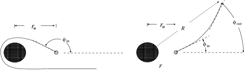
Figure 1: Photon path from radial coordinate $r_{0}$ to $R$. The path on the right indicates mild bending of the path due to spacetime curvature. On the left is shown the highly bent photon path which has an impact parameter near the critical value of photon capture, and a $\phi_{\rm out}$, at large $R$, of $2\pi$.

In a Schwarzschild hole with spacetime metric

$$ds^{2}=-\left(1-2M/r\right)dt^{2}+\left(1-2M/r\right)^{-1}dr^{2}+r^{2}\left(\ d\theta^{2}+\sin^{2}\theta\;d\phi^{2}\right)\,,$$ (1)

we consider a point at $r=r_{0}$, $\phi=0$, in the $\theta=\pi/2$ equatorial plane. At this point, a photon (i.e. , a null geodesic) with 4-momentum $p^{\mu}$ is emitted in the equatorial plane. From the fact that $p_{\phi}$ and $p_{0}$ are constants of motion for the equatorial photon, it follows that the photon orbit obeys

$$\frac{1}{r^{4}}\left(\frac{dr}{d\phi}\right)^{2}+\frac{1-2M/r}{r^{2}}=\frac{1}{b^{2}}\,,$$ (2)

where $b$ is the photon impact parameter.

We define $\phi_{\rm in}$ to be $\tan^{-1}({rp^{\phi}/p^{r}})$, the angle with respect to the outgoing direction, at which the photon is emitted. (Note that this differs from the angle $\tan^{-1}({rp^{\phi}/\sqrt{g_{rr}\;}p^{r}})$ that would be measured in the local frame of a coordinate stationary observer.) The value $\phi_{\rm in}$ is a constant characterizing the orbit, and is related to the impact parameter $b$ by Eq. (2) with $r$ set equal to $r_{0}$:

$$\frac{1}{\tan^{2}{\phi_{\rm in}}}+1-\frac{2M}{r_{0}}=\frac{r_{0}^{2}}{b^{2}}\,.$$ (3)

A critical value of the impact parameter is $b_{\rm crit}=3\sqrt{3\;}M$; for $b<b_{\rm crit}$, inward going photons will be captured by the hole. For any $r_{0}$, capture will occur if $|\phi_{\rm in}|>\phi_{\rm crit}$ where $\phi_{\rm crit}$ is the root, between $\pi/2$ and $\pi$, of

$$\tan{\phi_{\rm crit}}=-\,\left(\frac{r_{0}^{2}}{27M^{2}}-1+\frac{2M}{r_{0}}\right)^{-1/2}\,.$$ (4)

For $|\phi_{\rm in}|$ less than $\phi_{\rm crit}$, our universal functions relate the description of the photon at very large distance $R$ to its emission conditions. The first of these functions measures the bending of a photon trajectory, relative to the radially outgoing direction from its emission point. To define this function we start by defining ${\cal F}(\phi_{\rm in};R)$ to be the $\phi$ location, at large radius $R$, of a photon emitted at radius $r_{0}$, at angle $\phi_{\rm in}$ to the outgoing direction. We then define

$$F(\phi_{\rm in})=\lim_{R\rightarrow\infty}{\cal F}(\phi_{\rm in};R)\ .$$ (5)

The function $F$ is an odd function of $\phi_{\rm in}$; it is parametrized by $r_{0}/M$, but has no other dependencies. The second universal function $T$ is related to the coordinate time ${\cal T}(\phi_{\rm in};R)$ required for the the photon to reach asymptotically large $R$. To have the result be a finite value, we subtract the coordinate time to reach $R$ with $\phi_{\rm in}=0$, so that

$$T(\phi_{\rm in})\equiv\lim\limits_{R\rightarrow\infty}\left[{\cal T}(\phi_{\rm in};R)-{\cal T}(0;R)\right]\,,$$ (6)

and is an even function of $\phi_{\rm in}$; like $F$, it is parametrized by $r_{0}/M$, but has no other dependencies.

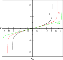
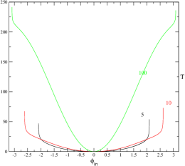
Figure 2: Universal functions $F$ and $T$. Curves are labeled with the values of $r_{0}/M$: 5, 10, and 100. The values of $\phi_{\rm crit}$, from Eq. (4) are respectively 2.0895, 2.6109, and 3.0896.

Plots of $F$ and $T$ are given in Fig. 2 for three values of $r_{0}/M$. Approximate fits to these curves, good both for small $\phi_{\rm in}$ and for $\phi_{\rm in}$ near $\phi_{\rm crit}$, are given by

$$F(\phi_{\rm in})=-{\rm sign}(\phi_{\rm in})\log\left(1-|\frac{\phi_{\rm in}|}{\phi_{\rm crit}}\right)-\frac{\phi_{\rm in}}{\phi_{\rm crit}}+\phi_{\rm in}$$ (7)

$$T(\phi_{\rm in})=r_{0}\left(1-\cos(\phi_{\rm in})\right)-{3\sqrt{3}}\log\left(1-\frac{|\phi_{\rm in}|}{\phi_{\rm crit}}\right)-\frac{3\sqrt{3}}{\phi_{\rm crit}}|\phi_{\rm in}|\,.\\$$ (8)

The details of the computation of these curves, and more accurate analytic approxmations to the curves, are given in Appendix B.

3 Pulse arrival times from universal functions

3.1 General case

We consider an emission event, at Schwarzschild radial coordinate $r_{0}$, and a photon emitted in the direction ${\mathbf{n}}$. We let $\alpha$ be the angle, as shown in Fig. 3, between the orbital plane and the plane containing the photon trajectory, i.e. , the plane defined by ${\mathbf{n}}$ and the radially outward direction. (If these directions coincide, we take $\alpha$ to be zero.)

We introduce a spatial triad of orthonormal vectors ${\mathbf{e}}_{x},{\mathbf{e}}_{y},{\mathbf{e}}_{z}$, with ${\mathbf{e}}_{x},{\mathbf{e}}_{y}$ in the pulsar orbital plane, and we define ${\mathbf{e}}_{x^{\prime}},{\mathbf{e}}_{y^{\prime}},{\mathbf{e}}_{z^{\prime}}$, to be the orthonormal spatial triad that result from a rotation by $\alpha$ around the outgoing direction ${\mathbf{e}}_{x}$, so that ${\mathbf{e}}_{x^{\prime}},{\mathbf{e}}_{y^{\prime}}$ lie in the plane of the photon trajectory.

To specify the direction of ${\mathbf{n}}$ we use the spherical polar angles $\phi_{0}$, $\beta_{0}$ with respect to the ${\mathbf{e}}_{x},{\mathbf{e}}_{y},{\mathbf{e}}_{z}$ directions. (Note that for convenience we are using the latitude $\beta$, rather than the more typical colatitude $\theta=\pi/2-\beta$.) From the rotational transformation between the unprimed and primed triads we get

$$\tan\alpha=\frac{\tan\beta_{0}}{\sin\phi_{0}}$$ (9)

$$\cos\phi_{\rm in^{\prime}}=\cos\beta_{0}\;\cos\phi_{0}\;.$$ (10)

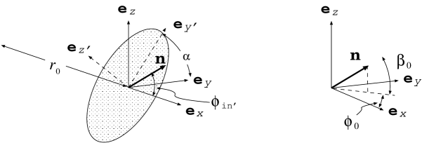
Figure 3: Triads and angles used to define photon directions.

Here $\phi_{\rm in^{\prime}}$ is the angle, in the plane of the photon trajectory, between the photon direction and the radially outgoing direction. We can, therefore, find $\phi_{\infty^{\prime}}$, the asymptotic $\phi$ direction, from

$$\phi_{\infty^{\prime}}=F(\phi_{\rm in^{\prime}})\ .$$ (11)

The spherical polar angles, in the ${\mathbf{e}}_{x},{\mathbf{e}}_{y},{\mathbf{e}}_{z}$ frame, for the final photon direction, are then

$$\cos\theta_{\infty}=\sin\alpha\sin\phi_{\infty^{\prime}}\quad\quad\quad\quad\tan{\phi_{\infty}}=\cos\alpha\tan{\phi_{\infty^{\prime}}}\,.$$ (12)

We summarize here the set of equations that give the final photon direction $\beta_{\infty},\phi_{\infty}$, and relative time of arrival $t_{\infty}$, in terms of the original photon direction $\beta_{0},\phi_{0}$:

$$\cos\phi_{\rm in^{\prime}} = \cos\beta_{0}\;\cos\phi_{0}$$ (13)

$$\sin\beta_{\infty} = \sin{\big{(}F(\phi_{\rm in^{\prime}})\big{)}}\,\frac{\sin\beta_{0}}{\sqrt{\sin^{2}\beta_{0}+\cos^{2}\beta_{0}\sin^{2}\phi_{0}\;}}$$ (14)

$$\tan\phi_{\infty} = \tan{\big{(}F(\phi_{\rm in^{\prime}})\big{)}}\,\frac{\cos\beta_{0}\sin\phi_{0}}{\sqrt{\sin^{2}\beta_{0}+\cos^{2}\beta_{0}\sin^{2}\phi_{0}\;}}$$ (15)

$$t_{\infty} = t_{e}+T(\phi_{\rm in^{\prime}})\ .$$ (16)

3.2 Special case: beaming in orbital plane

If the pulsar beam is emitted into the orbital plane, then $\beta_{0}=0$ and the relations in Eqs. (13)-(16) reduce to $\phi_{\rm in^{\prime}}=\phi_{0}$, and $\phi_{\infty}=F(\phi_{\rm in})$. The photon remains in the orbital plane, so $\beta_{\infty}=\beta_{0}=0$.

For the simplest example of strong field effects we restrict ourselves to the case in which the receiving antenna is precisely in the orbital plane of the pulsar. This means that photons reaching the antenna must have exceedingly small values of $\beta_{0}$ (of order of the antenna size divided by tens of kiloparsecs). In this case the initial-to-final transformations in Eqs. (13)-(16) can be replaced by approximations valid to first order in $\beta_{0}$:

$$\beta_{\infty} = \beta_{0}\;\frac{\sin\left(F(\phi_{0})\right)}{\sin\phi_{0}}$$ (17)

$$\phi_{\infty} = F(\phi_{0})\,.$$ (18)

In these equations it is assumed that $\beta_{0}\ll\phi_{0}$, a condition that will be violated only by photons directed very nearly radially outward, and hence experiencing no strong field effects. The sine function in the numerator of Eq. (17) implies $\beta_{\infty}=0$ if $F(\phi_{0})=\pi$. This corresponds to the case that all small-$\beta_{0}$ photons with the same value of $\phi_{0}$ are focused into the orbital plane, creating an intensity amplification that would be infinite aside from diffraction limitation.

Equations (17), (18) give us the factors by which strong field effects lead to convergence or divergence of the photon beam both in the pulsar orbital plane $f_{\rm plane}$, and perpendicular to it $f_{\rm perp}$:

$$f_{\rm plane}=\frac{dF}{d\phi_{0}}\quad\quad\quad f_{\rm perp}=\frac{\sin\left(F(\phi_{0})\right)}{\sin\phi_{0}}\,.$$ (19)

The total strong-field effect on the cross sectional area of the beam reaching the receiver is $f_{\rm plane}f_{\rm perp}$. The effect on the photon flux at the receiver will therefore be $1/\left(f_{\rm plane}f_{\rm perp}\right)$. The total radio intensity reaching the receiver will also depend on the gravitational redshift of the photons and the Doppler shift due to the motion of the emitting pulsar. Both effects are of order $M/r_{0}$.

4 Appearance and timing of pulses

We make another simplifying assumption: that the pulsar that emits its beam in the equatorial plane, is moving in a circular orbit at radius $r_{0}$. For definiteness we take the angular location of the pulsar to be given by $\phi_{\rm orb}=\Omega t$, where “$t$” here and below, indicates coordinate time. At a particular emission time $t_{\rm e}$, it is shown in Appendix A that the angle at which the photon is emitted is given by

$$\tan{\big{(}\phi_{\rm in}(t_{\rm e})\big{)}}=\frac{r_{0}\Omega\left(1-2M/r_{0}\right)^{-1/2}+\cos{({\gamma^{-1}[\Omega-\omega]}t_{\rm e}+\delta)}}{\gamma^{-1}\sin({\gamma^{-1}[\Omega-\omega]}t_{\rm e}+\delta)}\,.$$ (20)

Here $r_{0}$ is the radial coordinate of the circular orbit; $\Omega=\sqrt{M/r_{0}^{3}\;}$ is the pulsar orbital angular velocity (per unit coordinate time); $\omega$ is the pulsar spin rate as measured by a comoving observer; the Lorentz factor $\gamma$ is $1/\sqrt{1-3M/r_{0}\;}$; and $\delta$ is a phase constant specifying the direction of the beam at $t_{\rm e}=0$.

If a distant radio receiver is at $\phi_{\rm rec}$, then to find the emission time of photons that are destined to be received, we must solve

$$\Omega t_{\rm e}+F\big{(}\phi_{\rm in}(t_{\rm e})\big{)}=\phi_{\rm rec}\,.$$ (21)

Due to the nature of $F$ near the critical angles $\phi_{\rm crit}$, there are, in principle an infinite number of solutions corresponding to photon orbits that circle the gravitating center zero times, once, twice, etc. It will be useful to refer to these received pulses as primary, secondary (once around the gravitating center), tertiary, and so forth. We shall see, however, that these distinctions can become ambiguous.

The observationally important questions are the timing and appearance of the pulses that show strong field effects. We start by arguing that the effect on the pulse shape will be negligible if the rotation period (seconds or less) of the pulsar is much smaller than the pulsar orbital period (1000s of seconds to years, depending on $r_{0}/M$ and on the mass of the central supermassive black hole).

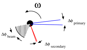
Figure 4: The pulsar beam sweeping through the narrow range of directions that connect to the receiver.

Figure 4 shows the geometry of beam emission, with $\Delta\phi_{\rm beam}$ indicating the inherent angular width (in the orbital plane) of the pulsar beam, and with $\Delta\phi_{\rm primary}$ and $\Delta\phi_{\rm secondary}$ indicating (but exaggerating) the receiver acceptance directions, i.e., the range of photon directions that connect to the distant radio receiver. The angular size of $\Delta\phi_{\rm primary}$ is approximately the ratio of the receiver diameter to the receiver distance. The much smaller angular size $\Delta\phi_{\rm secondary}$ is further divided by $dF/d\phi_{\rm in}$, a large number. For tertiary and subsequent beams, the same description applies except that the value of $dF/d\phi_{\rm in}$ is even larger.

If the pulsar were at a fixed coordinate position, and rotating at $\omega$, then the shape of the received pulse can be viewed as the result of the narrow cones of receiver acceptance sweeping through the $\Delta\phi_{\rm beam}$ beam profile. This viewpoint makes it clear that the time profile of the primary, secondary, etc. beams would have the same shape. The pulsar, of course, is not coordinate stationary, but is orbiting with orbital speed $\Omega$. This means that there will be a small change in the nature of $dF/d\phi_{\rm in}$ during the passage of the beam width through the receiver acceptance cones, since the value of $\phi_{\rm in}$ for received photons will change slightly during beam reception. To estimate this effect we can consider the change $\Delta F$ during the change in pulsar orbital location $\Delta\phi_{\rm orb}$:

$$\frac{dF}{d\phi_{\rm in}}\,\Delta\phi_{\rm in}\approx\frac{dF}{d\phi_{\rm in}}\,\Delta\phi_{\rm orb}\frac{\Omega}{\omega}\,.\approx e^{F}\,2\pi\,\frac{\Omega}{\omega}\,.$$ (22)

(The second approximations assumes that $\phi_{\rm in}\approx\phi_{\rm crit}$ and that $F$ is large.) For a secondary beam, $F$ must be of order $2\pi$; for a tertiary beam, $F$ must be order $4\pi$ etc. Thus, in the case of high order beams or for exceptionally large values of $\Omega/\omega$, there could be some distortion of received pulse shapes. This possibility will not be considered further in the current paper.

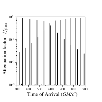
Figure 5: The factor $1/f_{\rm plane}$ for photon capture events from a pulsar with orbital radius $30\times GM/c^{2}$, and pulsar rotation rate 20.2 times the orbital rotation rate. Events for several orbits are shown on the left. Details are shown on the right for the orbital epoch during which the pulsar is on the far side of the hole.

Figure 5 shows a schematic of pulses emitted from a pulsar orbiting at a distance $30\times GM/c^{2}$ from a supermassive black hole of mass $M$. The pulsar rotation rate has been chosen to be very low, only 20.2 times the orbital frequency, in order to show clearly some of the phenomenology of the pulse arrival times. For a $4\times 10^{6}M_{\odot}$ black hole, this means an orbital period of $2\pi\times 30^{3/2}\times GM/c^{3}\approx 20,000$ seconds and a pulsar rotation period around 1000 seconds; an actual observed pulsar would likely be rotating hundreds or thousands of times faster. The horizontal axis represents the pulse arrival time (relative to an arbitrary start time), while the vertical axis gives the attenuation factor $1/f_{\mathrm{plane}}$ due to horizontal spreading of the beam. Using this factor as a tag on the pulses is useful in the discussion of the pulse sequences. The factor gives a rough indication of relative pulse strengths, though the full amplification or attenuation of the beam requires the complete spreading factor $1/f_{\mathrm{plane}}f_{\mathrm{perp}}$, and will be discussed below.

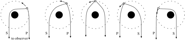
Figure 6: Prograde and retrograde photon trajectories. The pulsar is shown orbiting in the counterclockwise direction around a much more massive black hole. The leftmost cartoon shows that the observing radio telescope receives a primary (P) direct pulse and a highly bent secondary (S) pulse. The subsequent panels show trajectories as the pulsar continues its orbtial motion. The primary trajectory has increased bending and the secondary less, until the pulsar is directly opposite the receiver and the two trajectories are symmetric. The following panels shows how the prograde trajectory then becomes the primary (less bent) trajectory.

Initially, the taller set of pulses represents pulses that arrive at the detector from the pulsar along a more-or-less direct path. The initially weaker but strengthening set represents pulses that arrive from a path that is bent around the black hole in a sense prograde to the orbit. Figure 6 illustrates how this secondary path “unwinds” and becomes more direct as the pulsar moves along its orbit. The effective photon path length $\ell$ also shortens with time, giving rise to a shorter (blueshifted) pulse period $P=P_{0}(1+\dot{\ell}/c)$. Around time $600\times GM/c^{3}$, the pulsar passes behind the black hole (the middle panel in Fig. 6). After this, the prograde path becomes the more direct path, while what was formerly the more direct path now gets wound around the black hole in the retrograde sense, causing its pulses to weaken and the period of the pulses to redshift. The pulse timing near the time of this orbital phase is shown in greater detail in the second panel of Figure 5, where the prograde-wound pulses are shown in gray to distinguish them from the other pulses. The process repeats itself one orbit later. The ragged pulses at the bottom of the two graphs are pulses from paths with higher-order windings around the black hole; some of these will eventually unwind to become, for a time, the most direct path.

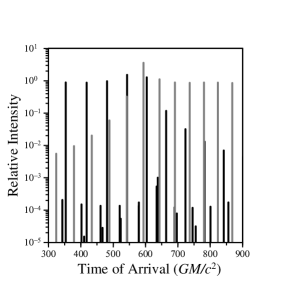
Figure 7: The relative intensity of pulses for the same system shown in Fig. 5

Figure 7 shows the same system, but with the vertical axis now showing the full pulse amplification (or attenuation) factor $1/f_{\mathrm{plane}}f_{\mathrm{perp}}$. Around the same time as the “primary” and “secondary” pulse trains swap roles, both sets of pulses go through a spike of amplification due to strong lensing around the black hole.

It should be understood that the “intensity” in Figure 7 and below refers to the photons received per unit time. The true energy intensity would include the effect of Doppler shifts due to the orbital motion. These effects, of order $r_{0}\Omega/c$, are significant – around 20% for an orbit with $r_{0}=30\times GM/c^{2}$ – but are omitted to emphasize the photon path effects.

The details of the pulse timing and amplification phenomenology depend on the orbital radius. To illustrate this, Fig. 8 shows the same information as Fig. 5 but for a more relativistic system, where the pulsar orbital radius is only $10\times GM/c^{2}$. Again, the pulsar rotation rate is taken to be artificially slow (only 47 times the orbital frequency) in order for the figure to show distinct pulses. In this more relativistic system, the pulse period shift, beaming asymmetry, and “tertiary” (multiply-wound) pulse paths are more apparent.

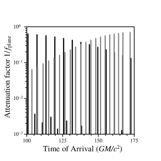
Figure 8: The same plot as in Fig. 5, but for a more relativistic system, with with orbital radius $10\times GM/c^{2}$, and with rotation rate 47 times the orbital frequency.

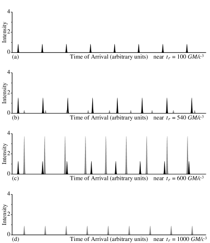
Figure 9: The appearance of received radio pulses for several orbital epochs of a pulsar orbiting with radius $30\times GM/c^{2}$. The pulsar rotation rate is assumed to be much greater than the orbital frequency.

Figure 9 shows the pulse trains that a radio astronomer might actually see from the $r_{0}=30\times GM/c^{2}$ system of Figs. 5 and 7, but assuming a more realistic pulsar rotation rate that is thousands of times faster than the orbital frequency. For such a sufficiently fast rotation rate, the pulsar orbital position changes negligibly during the emission of a set of a few pulses. The pulse intensity, determined by $F(\phi_{\rm in})$, and $dF/d\phi_{\rm in}$, and the red/blue shift in the period, determined by $\dot{\ell}$, therefore are fixed, once the orbital phase is fixed. This means that we can show pulse intensity and primary vs. secondary phase shifts without specifying any one pulsar rotation rate. For this reason, Fig. 9 does not specify units of the horizontal axis; it is understood that the spacing between direct pulses is the period of pulsar rotation. The time that is specified for each panel is the time that determines the orbital position when the set of pulses is emitted.

The vertical axis represents the pulse power relative to an undeflected beam, and each pulse is given a Gaussian shape. Panel (a) is a segment of the pulse train when the pulsar is on the near side of the black hole, and only a single train of direct pulses is visible. Panel (b) is a segment from the orbital phase during which the pulsar is passing behind the black hole: a secondary train of prograde-bent pulses, with blueshifted period, starts to appear. In panel (c), the prograde path has become the more direct path, and the pulses from what was originally the direct path are weakening, and their period redshifting, as the path becomes a bent retrograde one around the black hole (though both sets of pulses are amplified due to lensing). In panel (d), the original pulse train has disappeared almost entirely, leaving only the pulses from the newly-unwound path.

We note that when the most-direct path shifts from passing retrograde around the hole to prograde around the hole (see Fig. 6), there is a sudden jump in the frequency of the strongest pulse train, as the derivative of the effective path length $\dot{\ell}$ switches from lengthening to shortening. (Equivalently, in this geometry, a train of high-frequency “secondary” pulses rises up and replaces the low-frequency “primary” pulses.) This is the strong-field analog of the well-known cusp in the Shapiro time delay curve, where the time delay switches from increasing to decreasing; since the observed pulse period is multiplied by 1 plus the time derivative of the time delay $P_{\mathrm{obs}}=P_{0}(1+dT_{\mathrm{Shapiro}}/dt)$, this corresponds to a discontinuous jump in period. Unlike the case of the “standard” Shapiro delay, the discontinuity is finite even for a perfect alignment, since the deflecting mass is a black hole of finite size. There is also a slight asymmetry due to the special relativistic beaming (“headlight effect”) of the pulsar in its orbit.

5 Summary and Conclusions

We have introduced the problem of black hole effects on pulses from an orbiting pulsar. We have shown that in the case of a spherically symmetric (i.e., nonrotating) hole, the use of two “universal functions” removes the need for extensive computation of null geodesics. The universal function approach to computation has been used for a first exploration of the phenomena that might be encountered with pulses from a pulsar-hole system. This first exploration investigates pulse emission in the orbital plane, for a pulsar in circular orbit around a nonrotating hole.

Even for this highly simplified configuration we have found a number of interesting phenomena: (i) “Primary” pulses (pulses that travel from the pulsar to the receiver with relatively little gravitational bending) are continually accompanied by higher order (secondary, tertiary,…) pulses emitted during earlier pulsar orbits. (ii) As would be expected, the primary pulses do not have a constant period, but rather have a period that is modulated by orbital motion. (iii) The period of primary and of higher order pulses is not precisely the same, thus the higher order pulses arrive with a phase shift, relative to the primary pulses, that varies from one pulse to the next. (iv) Strong field effects dominate the pulsar observations when the pulsar is on the far side of the hole, the side opposite that of the receiver. In this case the emitted pulse can reach the receiver only by a highly bent path. (v) During the epoch of emission from the far side, the sequence of primary pulses and the sequence of secondary pulses, exchange roles. One consequence is that there is no clear distinction of primary and secondary for pulses emitted when the pulsar is close to the middle of its passage through the far side of the hole. (vi) For emission during most of the pulsar orbit, the secondary pulses have much lower intensity than the primary pulses. As the pulsar moves toward the dark side, however, the secondary pulses increase in intensity and the primary pulses decrease. (vii) Among the pulses emitted from the dark side are pulses that are amplified by strong field effects analogous to gravitational lensing.

The simple configuration studied would be expected to exaggerate strong field effects when compared to a more realistic configuration in which pulse emission is directed well out of the orbital plane. For example, if the pulsar spin axis is perpendicular to the orbital plane (as in our simple configuration), and emission is not close to the orbital plane (contrary to our simple configuration), the pulse trajectory will never cross the orbital plane, and hence never come sufficiently near the hole for strong field effects to be significant. More interesting is the case in which the spin axis and beaming details are such that the beam does cross (or pass close to) the orbital plane. Particularly noteworthy would be a configuration in which the receiver receives no primary pulses, and receives pulses only with the aid of strong field bending. It is also of note that some of the phenomena we have described, especially the existence of higher order pulses, can also occur in principle in binary pulsar systems, and pulsar-hole binaries of comparable mass.

Work is underway on investigating configuratins with out of orbit beaming. An exploration of the large parameter space will be feasible with the efficiency provided by the universal function approach, so we are, at least at first, restriciting attention to nonrotating supermassive holes.

6 Acknowledgment

We gratefully acknowledge support by the National Science Foundation under grants AST0545837, PHY0554367 and 0734800. We also thank the NASA Center for Gravitational Wave Astronomy at University of Texas at Brownsville. YW acknowledges support by the Chinese National Science Foundation under grant 10773005.

Appendix A Emission direction as a function of time

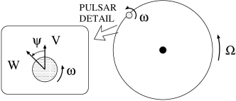
Figure 10: The figure illustrates the orbital motion of the pulsar at frequency $\Omega$, the parallel transported spatial direction $V^{\mu}$, and the pulsar beam direction $W^{\mu}$ rotating at frequency $\omega$ relative to $V^{\mu}$, as observed in a frame comoving with the pulsar.

In the orbital plane we let the angular position of the pulsar be $\phi=\Omega t$, with $t$ the Scharzschild coordinate time and the pulsar’s 4-velocity components are

$$U^{0}=\gamma\quad\quad U^{\phi}=\gamma\Omega$$ (A1)

where

$$\gamma=\frac{1}{\sqrt{1-2M/r_{0}-r_{0}^{2}\Omega^{2}\;}}=\frac{1}{\sqrt{1-3M/r_{0}\;}}\ .$$ (A2)

We let $V^{\mu}$ be a 4-vector that is spatial (that is, orthogonal to $U^{\mu}$), that has no component out of the equatorial orbital plane, and that is parallel transported around with the pulsar. (Since the pulsar world line is a geodesic, this is the same as Fermi-Walker transporting $V^{\mu}$.) It is straightforward to show that the components of such an “inertial direction” are

$$V^{r}=\gamma^{-1}{r_{0}}K\sin{(\gamma^{-1}{\Omega}t+\delta)}\quad\quad V^{\phi}=K\cos{(\gamma^{-1}{\Omega}t+\delta)}\quad\quad V^{0}=\frac{r_{0}^{2}\Omega}{{1-2M/r_{0}\;}}K\cos{(\gamma^{-1}{\Omega}t+\delta)}\,.$$ (A3)

where $K$ is a scaling constant and $\delta$ is a phase factor determining the direction in which $V^{\mu}$ is pointing at $t=0$. We let $W^{\mu}$ be a spatial vector, in the equatorial plane, that points in the direction of the pulsar beam. We let $\psi$ be the angle, measured in the positive sense (the positive sense for $\Omega$) from $V^{\mu}$ to $W^{\mu}$. In terms of the proper time $\tau$ measured by the pulsar, we define the locally observed pulsar spin rate $\omega$ by

$$\psi=\omega\tau=\omega t/\gamma\,.$$ (A4)

From $W^{\mu}U_{\mu}=0$ and $\cos{\psi}=W^{\mu}V_{\mu}/VW$ we get

$$W^{r}=\frac{A}{\gamma}\sin{(\gamma^{-1}{[\Omega-\omega]}t+\delta)}\quad\quad W^{\phi}=\frac{A}{r_{0}}\cos{(\gamma^{-1}{[\Omega-\omega]}t+\delta)}$$

$$W^{0}=\frac{r_{0}\Omega A}{{1-2M/r_{0}\;}}\cos{(\gamma^{-1}{[\Omega-\omega]}t+\delta)}\,.$$ (A5)

In the comoving frame of the pulsar the spatial direction of the photon beam is $W^{\mu}$, thus the photon 4-momentum must have the form $\vec{p}=\kappa\vec{U}+\vec{W}$. The value of $\kappa$ follows from $p^{\mu}p_{\mu}=0$ and we find

$$\vec{p}=\frac{A}{\gamma\sqrt{1-2M/r_{0}\;}}\,\vec{U}+\vec{W}\,,$$ (A6)

from which we get the components

$$p^{0} = \frac{A}{\sqrt{1-2M/r_{0}\;}}+\frac{r_{0}\Omega A}{{1-2M/r_{0}\;}}\cos{(\gamma^{-1}{[\Omega-\omega]}t+\delta)}$$ (A7)

$$p^{\phi} = \frac{A\Omega}{\sqrt{1-2M/r_{0}\;}}+\frac{A}{r_{0}}\cos{(\gamma^{-1}{[\Omega-\omega]}t+\delta)}$$ (A8)

$$p^{r} = \gamma^{-1}{A}\sin{(\gamma^{-1}{[\Omega-\omega]}t+\delta)}\,.$$ (A9)

This tells us that the photon starts out its journey with

$$\frac{p^{r}}{p^{\phi}}=\frac{dr}{d\phi}=\frac{r_{0}\gamma^{-1}\sin({\gamma^{-1}[\Omega-\omega]}t+\delta)}{\frac{r_{0}\Omega}{\sqrt{1-2M/r_{0}\;}}+\cos{({\gamma^{-1}[\Omega-\omega]}t+\delta)}}\,,$$ (A10)

with

$$\frac{p^{r}}{p^{0}}=\frac{dr}{dt}=\frac{\gamma^{-1}\sin({\gamma^{-1}[\Omega-\omega]}t+\delta)}{\frac{1}{\sqrt{1-2M/r_{0}\;}}+\frac{r_{0}\Omega}{1-2M/r_{0}}\cos{({\gamma^{-1}[\Omega-\omega]}t+\delta)}}\,,$$ (A11)

and with

$$\frac{p^{\phi}}{p^{0}}=\frac{d\phi}{dt}=\frac{\frac{\Omega}{\sqrt{1-2M/r_{0}\;}}+\frac{1}{r_{0}}\cos{(\gamma^{-1}{[\Omega-\omega]}t+\delta)}}{\frac{1}{\sqrt{1-2M/r_{0}\;}}+\frac{r_{0}\Omega}{1-2M/r_{0}}\cos{(\gamma^{-1}{[\Omega-\omega]}t+\delta)}}\,.$$ (A12)

Equation (20) follows from Eq. (A10) and from the definition of $\tan{\phi_{\rm in}}$ as the initial value of $rd\phi/dr$.

Appendix B Computation of the universal functions

B.1 Integral for $\phi_{\infty}$

For a photon beamed in the equatorial plane, we assume that we know its initial radial location $r_{0}$ and its initial direction, as specified by the angle measured with respect to the outgoing radial direction

$$\phi_{\rm in}=\tan^{-1}{\left(r_{0}d\phi/dr\right)}\,.$$ (B1)

The equation for the photon orbit is

$$\frac{1}{r^{4}}\left(\frac{dr}{d\phi}\right)^{2}+\frac{1-2M/r}{r^{2}}=\frac{1}{b^{2}}\ .$$ (B2)

From the known initial values of $r$ and of $dr/d\phi$ we solve Eq. (B2) for the impact parameter $b$, a constant of motion for the orbit. We proceed with the following steps to find $\phi_{\infty}$. In the following we describe as “delicate” any integral that has a divergent integrand, and for which special techniques, desribed in Appendix B.3, must be used.

1. Suppose $\cos{(\phi_{\rm in})}>0$, so that the photon is emitted going generally outward. In this case the photon will be moving only to larger $r$, but it may be moving to larger or smaller $\phi$, and we must separate this case into two subcases depending on the initial value of $dr/d\phi$:

   1. If initially $dr/d\phi>0$, then we use

      $${\phi}_{\infty}(t)=\Omega t+\int_{r_{0}}^{\infty}\frac{dr}{\sqrt{r^{4}/b(t)^{2}-r^{2}+2Mr\;}}\ .$$ (B3)

   2. If initially $dr/d\phi<0$ we use

      $${\phi}_{\infty}(t)=\Omega t-\int_{r_{0}}^{\infty}\frac{dr}{\sqrt{r^{4}/b(t)^{2}-r^{2}+2Mr\;}}\ .$$ (B4)

   In both these cases, the integrands do not diverge, and no special techniques are needed to carry out the integration.

2. If $\cos{\phi_{\rm in}}=0$ it means that the photon is emitted on a trajectory tangent to the pulsar orbit. In this case we must check whether the the photon is going in the direction of increasing or decreasing $\phi$:

   1. If $\sin{\phi_{\rm in}}>0$, then we use Eq. (B3).

   2. If $\sin{\phi_{\rm in}}<0$, then we use Eq. (B4).

   In the $\cos{\phi_{\rm in}}=0$ case, either of the integrals is “delicate” since the integrand diverges at $r=r_{0}$.

3. If $\cos{(\phi_{\rm in})}<0$ and if $b^{2}>27M^{2}$, then there will be a value of $r$, less than $r_{0}$, at which $dr/d\phi=0$, i.e., at which the denominator of the integrand in Eq. (B3) vanishes. Call that value $r_{\rm min}$. Then we need to consider the usual subcases:

   1. If $\sin{(\phi_{\rm in})}>0$, then

      $${\phi}_{\infty}(t)=\Omega t+2\int_{r_{\rm min}}^{r_{0}}\frac{dr}{\sqrt{r^{4}/b(t)^{2}-r^{2}+2Mr\;}}+\int_{r_{0}}^{\infty}\frac{dr}{\sqrt{r^{4}/b(t)^{2}-r^{2}+2Mr\;}}\,.$$ (B5)

   2. If $\sin{(\phi_{\rm in})}<0$, then

      $${\phi}_{\infty}(t)=\Omega t-2\int_{r_{\rm min}}^{r_{0}}\frac{dr}{\sqrt{r^{4}/b(t)^{2}-r^{2}+2Mr\;}}-\int_{r_{0}}^{\infty}\frac{dr}{\sqrt{r^{4}/b(t)^{2}-r^{2}+2Mr\;}}\,.$$ (B6)

4. If $\cos{(\phi_{\rm in})}<0$ and if $b^{2}<27M$, then the photon will be captured by the black hole and there is no meaning to ${\phi_{\infty}}$.

B.2 Integral for time to infinity

We need to find the coordinate time it takes for a photon to reach “infinity.” The calculation must be divided into two subcases depending on whether the photon starts going outward ($\cos{(\phi_{\rm in})}>0$) or inward ($\cos{(\phi_{\rm in})}<0$). In both cases the calculation is based on the equation for $dr/dt$ for the photon motion (see MTW, Eqs. 25.64 and 25.66):

$$\frac{dt}{dr}=\frac{1}{b(1-2M/r)}\,\frac{1}{\sqrt{\frac{1}{b^{2}}-\frac{1}{r^{2}}+\frac{2M}{r^{3}}\;}}\equiv J(r)\ .$$ (B7)

1. If the photon starts its trajectory at time $t_{e}$, with $\cos{(\phi_{\rm in})}>0$, then the photon will always be traveling outward and

   $$t_{\infty}=t_{e}+\int_{r_{0}}^{\infty}J(r)dr\,.$$ (B8)

   In this case the integral is not delicate.

2. If the photon starts its trajectory with $\cos{(\phi_{\rm in})}=0$, then Eq. (B8) again applies, but now the integral is delicate, since $f(r_{0})$ is infinite.

3. If the photon starts its trajectory with $\cos{(\phi_{\rm in})}<0$, then let $r_{\rm min}$ have the same meaning as in Eq. (B5) (B6). The time of arrival of the pulse is now given by

   $$t_{\infty}=t_{e}+2\int_{r_{\rm min}}^{r_{0}}J(r)dr+\int_{r_{0}}^{\infty}J(r)dr\,.$$ (B9)

   The first integral is delicate since $J(r_{\rm min})$ is infinite.

B.3 Computational details for integrals

The integrals for $\phi_{\infty}$ and $t_{\infty}$ cannot in general be expressed as elementary functions, and must be handled by numerical methods. If there is no singularity in the integrand, such as in the case $\cos(\phi_{\rm in})>0$, we use adaptive Simpson quadrature with an absolute error limit set at $10^{-6}$.

In the case that the integrand does diverge, the divergences occur at the a root of the polynomial $r^{3}-b^{2}r+2Mb^{2}$. For $b^{2}<27M^{2}$ this polynomial has a negative root and two postive roots. We denote the largest root as $r_{\rm min}$ since it is the minimum radius the photon trajectory will reach. We then write

$$r^{4}/b^{2}-r^{2}+2Mr=(r-r_{\rm min})f(r)$$ (B10)

where $f={r^{2}}(r+r_{\rm min})/b^{2}-2M{r}/{r_{\rm min}}$ does not vanish in the intervals of integration that are considered.

The use of this is illustrated for one of the integrals occurring in Eqs. (B5) and (B6):

$$I\equiv\int_{r_{min}}^{r_{0}}\frac{dr}{\sqrt{r^{4}/b^{2}-r^{2}+2Mr}}=\int_{r_{\rm min}}^{r_{0}}\frac{dr}{\sqrt{r-r_{\rm min}}\sqrt{f(r)}}$$ (B11)

$$=\int_{r_{\rm min}}^{r_{0}}\frac{dr}{\sqrt{r-r_{\rm min}}\sqrt{f(r_{\rm min})}}+\int_{r_{\rm min}}^{r_{0}}\frac{dr}{\sqrt{r-r_{\rm min}}}\left[\frac{1}{\sqrt{f(r)}}-\frac{1}{\sqrt{f(r_{\rm min})}}\right]$$

$$=\int_{r_{\rm min}}^{r_{0}}\frac{dr}{\sqrt{r-r_{\rm min}}\sqrt{f(r_{\rm min})}}+\int_{r_{\rm min}}^{r_{0}}\frac{dr}{\sqrt{r-r_{\rm min}}}\left[\frac{f(r_{\rm min})-f(r)}{\left(\sqrt{f(r_{\rm min})}+\sqrt{f(r)}\;\right)\sqrt{f(r_{\rm min})}\sqrt{f(r)}}\right]\ .$$

The numerator in the second integrand is

$$f(r_{\rm min})-f(r)=-\frac{1}{b^{2}}(r-r_{\rm min})(r^{2}+2r_{\rm min}r+2r_{\rm min}^{2}-2b^{2}M/r_{\rm min})\ .$$ (B12)

so that the evaluation of $I$ is reduced to

$$I=2\frac{\sqrt{r_{0}-r_{\rm min}}}{\sqrt{f(r_{\rm min})}}-\frac{1}{b^{2}\sqrt{f(r_{\rm min})}}\int_{r_{\rm min}}^{r_{0}}\frac{\sqrt{r-r_{\rm min}}(r^{2}+2r_{\rm min}r+2r_{\rm min}^{2}-2b^{2}M/r_{\rm min})dr}{(\sqrt{f(r_{\rm min})}+\sqrt{f(r)})\sqrt{f(r)}}\ .$$ (B13)

The remaining integral is nonsingular and can be evaluated e.g., with an adaptive Simpson’s routine.

An additional complication arises if $b^{2}$ is very close to $27M^{2}$. In this case the two positive roots of $f(r)$ approach each other, and the integral becomes very large. To deal with this case we introduce the notation $r_{2}$ for the smaller positive root and $r_{3}$ for the negative root, and we write

$$I\equiv\int_{r_{\rm min}}^{r_{0}}\frac{dr}{\sqrt{r^{4}/b^{2}-r^{2}+2Mr}}=b\int_{r_{\rm min}}^{r_{0}}\frac{dr}{\sqrt{r_{\rm min}(r_{\rm min}-r_{3})(r-r_{\rm min})(r-r_{2})}}\hskip 72.26999pt$$

$$\hskip 72.26999pt+b\int_{r_{\rm min}}^{r_{0}}\left[\frac{dr}{\sqrt{r(r-r_{3})(r-r_{\rm min})(r-r_{2})}}-\frac{dr}{\sqrt{r_{\rm min}(r_{\rm min}-r_{3})(r-r_{\rm min})(r-r_{2})}}\right]$$

$$=\frac{b}{\sqrt{r_{\rm min}(r_{\rm min}-r_{3})}}\left\{\int_{r_{\rm min}}^{r_{0}}\frac{dr}{\sqrt{(r-r_{\rm min})(r-r_{2})}}-\int_{r_{\rm min}}^{r_{0}}\frac{\sqrt{r-r_{\rm min}}(r+r_{\rm min}-r_{3})\;dr}{\left(\sqrt{r_{\rm min}(r_{\rm min}-r_{3})}+\sqrt{r(r-r_{3})}\,\right)\sqrt{r(r-r_{3})(r-r_{2})}}\right\}$$

$$=\frac{b}{\sqrt{r_{\rm min}(r_{\rm min}-r_{3}})}\left\{2\log\left(\frac{\sqrt{r_{0}-r_{\rm min}}+\sqrt{r_{0}-r_{2}}}{\sqrt{r_{\rm min}-r_{2}}}\right)-\int_{r_{\rm min}}^{r_{0}}\frac{\sqrt{r-r_{\rm min}}(r+r_{\rm min}-r_{3})\;dr}{\left(\sqrt{r_{\rm min}(r_{\rm min}-r_{3})}+\sqrt{r(r-r_{3})}\right)\sqrt{r(r-r_{3})(r-r_{2})}}\right\}$$ (B14)

The remaining integrand is well behaved at $r=r_{\rm min}$ and is straightforward to evaluate numerically.

To get asymptotic approximations for $\phi_{\rm in}$ near $\phi_{\rm crit}$ we take $b^{2}=27M^{2}+\epsilon$, and we find that $r_{\rm min}\approx 3M+\sqrt{\epsilon\;}/3$ and $r_{2}\approx 3M-\sqrt{\epsilon\;}/3$. If we set $\phi_{\rm in}=\phi_{\rm crit}-\Delta\phi$, and assume positive $\phi_{\rm in}$ then from Eqs. (3) and (4) we find that $\Delta\phi\propto\epsilon$ and hence $\Delta\phi\propto(r_{\rm min}-r_{2})^{2}.$ The logarithmic dependence in Eq. (B14) becomes

$$\log(1/\sqrt{r_{\rm min}-r_{2}\;})\approx\log{\Delta\phi}\approx-\textstyle{\frac{1}{4}}\log(1-\phi_{\rm in}/\phi_{\rm crit})\ .$$ (B15)

The prefactor of the logarithm in Eq. (B14) is evaluated to 2 when the approximations $b=3\sqrt{b}$, $r_{\rm min}=r_{2}=3M$, $r_{3}=-6M$ are used, and we get the asymptotic approximation $-\frac{1}{2}\log{(1-\phi_{\rm in}/\phi_{\rm crit})}$. The first term in Eq. (7) follows from using this asymptotic approximation for Eq. (B14) in Eq. (B5) and modifying the result to make it an odd function of $\phi_{\rm in}$. The remaining terms are added to Eq. (7) to give $F(\phi_{\rm in})\approx\phi_{\rm in}$ for small $\phi_{\rm in}$. Equation  (7), therefore, gives the right qualitative behavior of $F(\phi_{\rm in})$ both for $\phi_{\rm in}\rightarrow 0$ and $\phi_{\rm in}\rightarrow\phi_{\rm crit}$.

The approximation for $T(\phi_{\rm in})$ in Eq. (7) follows from similar considerations with the addition of a Roemer time delay $r_{0}(1-\cos{\phi_{\rm in}})$, the time it takes the pulsar signal (with $c=1$) to cross the orbit on its way to the receiver. The appearance of this effect is clear in the $r_{0}=100M$ curve for $T(\phi_{\rm in})$ in Fig. 2.

It has been useful to have more accurate approximations to the universal functions than the expressions in Eqs. (7) and (8). To that end we have fit the errors (differences from the numerical integrals) in Eqs. (7) and (8) with even-order Chebyshev polynomials. The following polynomials give better than 1% fits to the numerical calculations when used with the coefficients in Table 1:

$$F(\phi_{\rm in})=-{\rm sign}(\phi_{\rm in})\left[\log(1-\frac{|\phi_{\rm in}|}{\phi_{\rm crit}})+f_{2}\phi_{\rm in}^{2}+f_{4}\phi_{\rm in}^{4}+f_{6}\phi_{\rm in}^{6}+f_{8}\phi_{\rm in}^{8}\right]-\frac{\phi_{\rm in}}{\phi_{\rm crit}}+\phi_{\rm in}$$ (B16)

$$T(\phi_{\rm in})=r_{0}(1-\cos{\phi_{\rm in}})-{3\sqrt{3}}\;\log(1-\frac{|\phi_{\rm in}|}{\phi_{\rm crit}})-\frac{3\sqrt{3}}{\phi_{\rm crit}}\;|\phi_{\rm in}|+t_{2}\phi_{\rm in}^{2}+t_{4}\phi_{\rm in}^{4}+t_{6}\phi_{\rm in}^{6}+t_{8}\phi_{\rm in}^{8}+t_{10}\phi_{\rm in}^{10}\,.$$ (B17)

Table 1: Coefficients of residual of universal function F and T

$r_{0}(M)$	$\phi_{\rm crit}$	$f_{2}$	$f_{4}$	$f_{6}$	$f_{8}$	$t_{2}$	$t_{4}$	$t_{6}$	$t_{8}$	$t_{10}$
5	2.0895	0.0634022	-0.0707841	0.0160038	-0.000411158	-0.86385	0.930642	-0.160082	0.00547166	0.0
10	2.6109	0.0171645	0.00324181	-0.000180664	0.000315048	-0.263976	0.599057	-0.115977	0.00609665	0.0
30	2.9677	-0.0352832	0.0569467	-0.0110258	0.000910931	-0.414603	0.786804	-0.212809	0.0236697	-0.00100843
100	3.0896	-0.128706	0.134169	-0.0274787	0.00192051	-0.884133	0.929001	-0.23247	0.0249892	-0.00103073

References

- Detweiler (1979) Detweiler, S. 1979, ApJ, 234, 1100
- Eisenhauer et al. (2005) Eisenhauer, F., Genzel, R., Alexander, T., Abuter, R., Paumard, T., Ott, T., Gilbert, A., Gillessen, S., Horrobin, M., Trippe, S., Bonnet, H., Dumas, C., Hubin, N., Kaufer, A., Kissler-Patig, M., Monnet, G., Ströbele, S., Szeifert, T., Eckart, A., Schödel, R., & Zucker, S. 2005, ApJ, 628, 246
- Estabrook & Wahlquist (1975) Estabrook, F. B., & Wahlquist, H. D. 1975, General Relativity and Gravitation, 6, 439
- Ghez et al. (2005) Ghez, A. M., Salim, S., Hornstein, S. D., Tanner, A., Lu, J. R., Morris, M., Becklin, E. E., & Duchêne, G. 2005, ApJ, 620, 744
- Ghez et al. (2008) Ghez, A. M., Salim, S., Weinberg, N. N., Lu, J. R., Do, T., Dunn, J. K., Matthews, K., Morris, M., Yelda, S., Becklin, E. E., Kremenek, T., Milosavljevic, M., & Naiman, J. 2008, ArXiv e-prints
- Levin (2007) Levin, Y. 2007, MNRAS, 374, 515
- Lu et al. (2006) Lu, J. R., Ghez, A. M., Hornstein, S. D., Morris, M., Matthews, K., Thompson, D. J., & Becklin, E. E. 2006, Journal of Physics Conference Series, 54, 279
- Maness et al. (2007) Maness, H., Martins, F., Trippe, S., Genzel, R., Graham, J. R., Sheehy, C., Salaris, M., Gillessen, S., Alexander, T., Paumard, T., Ott, T., Abuter, R., & Eisenhauer, F. 2007, ApJ, 669, 1024
- Misner et al. (1973) Misner, C. W., Thorne, K. S., & Wheeler, J. A. 1973, Gravitation (San Francisco: Freeman)
- Nayakshin & Sunyaev (2005) Nayakshin, S., & Sunyaev, R. 2005, MNRAS, 364, L23
- Sazhin (1978) Sazhin, M. V. 1978, Soviet Astronomy, 22, 36
- Verbiest et al. (2008) Verbiest, J. P. W., Bailes, M., van Straten, W., Hobbs, G. B., Edwards, R. T., Manchester, R. N., Bhat, N. D. R., Sarkissian, J. M., Jacoby, B. A., & Kulkarni, S. R. 2008, ApJ, 679, 675