An Ensemble Kalman-Particle Predictor-Corrector Filter for Non-Gaussian Data Assimilation

Abstract

An Ensemble Kalman Filter (EnKF, the predictor) is used make a large change in the state, followed by a Particle Filer (PF, the corrector), which assigns importance weights to describe a non-Gaussian distribution. The importance weights are obtained by nonparametric density estimation. It is demonstrated on several numerical examples that the new predictor-corrector filter combines the advantages of the EnKF and the PF and that it is suitable for high dimensional states which are discretizations of solutions of partial differential equations.

Key words: Dynamic data driven application systems, data assimilation, ensemble Kalman filter, particle filter, tracking, non-parametric density estimation, Bayesian statistics

1 Introduction

Dynamic Data Driven Application Systems (DDDAS) [1] aim to integrate data acquisition, modeling, and measurement steering into one dynamic system. Data assimilation is a statistical technique to modify model state in response to data and an important component of the DDDAS approach. Models are generally discretizations of partial differential equations and they may have easily millions of degrees of freedom. The model equations themselves are posed in functional spaces, which are infinitely dimensional. Because of nonlinearities, the probability distribution of the state is usually non-Gaussian.

A number of methods for data assimilation exist [2]. Filters attempt to find the best estimate from the model state and the data up to the present. We present a combination of the Ensemble Kalman Filter (EnKF) [3] and the Sequential Importal Sampling (SIS) particle filter (PF) [4]. The EnKF is a Monte-Carlo implementation of the Kalman Filter (KF). The KF is an exact method for Gaussian distributions. However, it needs to maintain the state covariance matrix, which is not possible for large state dimension. The EnKF and its variants [6, 7] replace the covariance by the sample covariance computed from an ensemble of simulations. Each ensemble member is advanced in time by the model independently until analysis time, when the data is injected, resulting in changes in the states of the ensemble members. Particle filters also evolve a ensemble of simulations, but they assign to each ensemble member a weight and the analysis step updates the weights.

The KF and the EnKF represent the probability distributions by the mean and the covariance, and so they assume that the distributions are Gaussian. This shows in the tendency of EnKF to smear distributions towards unimodal, as illustrated in Sec. 3 below. So, while the EnKF has the advantage that it can make large charges in the state and the ensemble can represent an arbitrary distribution, the EnKF is still essentialy limited to Gaussian distributions. On the other hand, the PF can represent non-Gaussian distributions faithfully, but it only updates the weights and cannot move ensemble members in the state space. Thus a method that combines the advantages of both without the disadvantages of either is of interest. The design of more efficient non-Gaussian filters for large-scale problems has been the subject of significant interest, often using Gaussian mixtures and related approaches [8].

The predictor-corrector filter presented here uses an EnKF as a predictor to move the state distribution towards the correct region and then a PF as corrector to adjust for a non-Gaussian character of the distribution. Nonparametric density estimation is used to compute the weights in the PF. The combined predictor-corrector method appears to work well on problems where either EnKF of PF fails, and it does not degrade the performace of the EnKF for Gaussian distributions. Predictor-corrector filters were first formulated in [9, 10]. Related results and some probabilistic background can be found in [11].

2 Formulation of the Method

A common procedure to construct an initial ensemble is as a sum with random coefficients [12],

$$u=\sum_{n=1}^{m}\lambda_{n}d_{n}\varphi_{n},\quad d_{n}\sim N\left(0,1\right),\quad\left\{d_{n}\right\}\text{ independent},$$ (1)

where $\left\{\varphi_{n}\right\}$ is an orthonormal basis in the space state $V=\mathbb{R}^{m}$ equipped with the Euclidean norm $\left\|\cdot\right\|$. The elements of $V$ are column vectors of values of functions on a mesh in the spatial domain. The basis functions $\varphi_{n}$ are smooth for small $n$ and more oscillatory for large $n$. If the the coefficients $\lambda_{n}\rightarrow 0$ sufficiently fast, the series (1) converges and $u$ is a random smooth function in the limit as $m\rightarrow\infty$. The sum (1) defines a Gaussian random variable with the eigenvalues of its covariance matrix equal to $\lambda_{k}^{2}$. Possible choices of $\left\{\varphi_{k}\right\}$ include a Fourier basis, such as the sine or cosine functions, or bred vectors [2]. On the state space $V$, we define another norm by

$$\left\|u\right\|_{U}^{2}=\sum_{n=1}^{m}\frac{1}{\kappa_{n}^{2}}c_{n}^{2},\quad u=\sum_{n=1}^{m}c_{n}\varphi_{n}.$$ (2)

Note that if $\kappa_{n}=1$, $\left\|\cdot\right\|_{U}$ is just the original norm $\left\|\cdot\right\|$ on $V$. We generally use $\kappa_{n}$ adapted to the smoothness of the functions in the initial ensemble, $\lambda_{n}/\kappa_{n}\rightarrow 0$ as $n\rightarrow\infty$.

A weighted ensemble of $N$ simulations $\left(u_{k},w_{k}\right)_{k=1}^{N}$ is initialized according to (1), with equal weights $w_{k}=1/N$. The ensemble members are advanced by the model and at given points in time, new data is injected by an analysis step. The data consists of vector $d$ of measurements, observation function $h\left(u\right)=Hu$, also called forward operator, here assumed to be linear, which links the model state space with the data space, and data error distribution, here assumed to be Gaussian with zero mean and known covariance $R$. The value of the observation function $Hu$ is what the data vector would be in the absence of model and data errors. The value of the probability density of the data error distribution at the data vector $d$ for a given value of the observation function $Hu$ is called data likelihood and denoted by $p(d|u)$. The probability distribution of the model state before the data is injected is called the prior or the forecast, and the distribution after the data is injected is called the posterior or the analysis. Assuming the forecast probability distribution has the density $p^{f}$, the density $p^{a}$ of the analysis is found from the Bayes theorem,

$$p^{a}\left(u\right)\propto p\left(d|u\right)p^{f}\left(u\right),$$ (3)

where $\propto$ means proportional.

Instead of working with densities, the probability distributions are approximated by weighted ensembles. We will call the following analysis step algorithm EnKF-SIS.

Predictor. Given a forecast ensemble

$$\left(u_{k}^{f},w_{k}^{f}\right)_{k=1}^{N},\quad w_{k}^{f}\geq 0,\quad\sum_{k=1}^{N}w_{k}^{f}=1,$$

the members $u_{k}^{a}$ of the analysis ensemble are found from the EnKF,

$$u_{k}^{a}=u_{k}^{f}+K(d_{k}-Hu_{k}^{f}),\quad d_{k}\sim N\left(d,R\right),\quad K=QH^{\mathrm{T}}\left(HQH^{\mathrm{T}}+R\right)^{-1}$$

where $d_{k}$ are randomly sampled from the data distribution, and $Q$ is the forecast ensemble covariance,

$$Q=\sum_{k=1}^{N}w_{k}\left(u_{k}-\overline{u}^{f}\right)\left(u_{k}-\overline{u}^{f}\right)^{\mathrm{T}},\quad\overline{u}^{f}=\sum_{k=1}^{N}w_{k}^{f}u_{k}^{f}.$$ (4)

This is the EnKF from [3], extended to weighted ensembles by the use of the weighted sample covariance (4).

Corrector. The analysis members $u_{k}^{a}$ are thought of as a sample from some proposal distribution, with density $p^{p}$. Ideally, the analysis weights $w_{k}^{a}$ should be computed from the SIS update as [4]

$$w_{k}^{a}\propto p\left(d|u_{k}^{a}\right)\frac{p^{f}\left(u_{k}^{a}\right)}{p^{p}\left(u_{k}^{a}\right)}.$$

However, the ratio of the densities is not known, so it is replaced by a noparametric estimate inspired by [13], giving

$$w_{k}^{a}\propto p\left(d|u_{k}^{a}\right)\frac{\sum_{\ell:\left\|u_{\ell}^{f}-u_{k}^{a}\right\|_{U}\leq h_{k}}w_{k}^{f}}{\sum_{\ell:\left\|u_{\ell}^{a}-u_{k}^{a}\right\|_{U}\leq h_{k}}\frac{1}{N}},\quad\sum_{k=1}^{N}w_{k}^{a}=1.$$

The bandwidth $h_{k}$ is the distance from $u_{k}^{a}$ to the $\lfloor N^{1/2}\rfloor$-th nearest member $u_{\ell}^{a}$, measured in the $\left\|\cdot\right\|_{U}$ norm.

3 Numerical Results

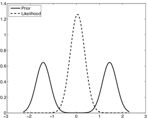
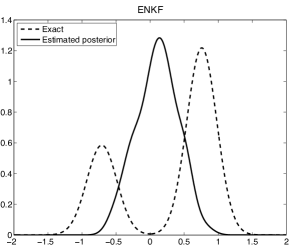
(a) Prior and data likelihood densities	(b) Posterior from EnKF
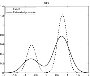
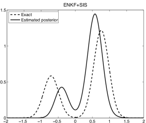
(c) Posterior from SIS	(d) Posterior from EnKF-SIS

Figure 1: Data assimilation with bimodal prior. EnKF fails to capture the non-Gaussian features of the posterior, but both SIS and EnKF-SIS represent the nature of the posterior reasonably well.

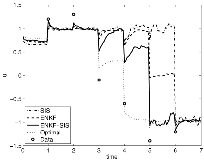
Figure 2: Ensemble filters mean and optimal filter mean for stochastic ODE (5). EnKF-SIS was able to approximate the optimal solution better than either SIS or EnKF alone.

Fig. 1 demonstrates a failure of EnKF for non-Gaussian distributions, while SIS and EnKF-SIS do fine. We construct a bimodal prior in 1D by first sampling from $N\left(0,5\right)$ and assigning the weights by

$$w_{f}(x_{i})=e^{-5(1.5-x_{i})^{2}}+e^{-5(-1.5-x_{i})^{2}}.$$

The data likelihood is Gaussian. The ensemble size was $N=100$.

The next 1D problem demonstrates that EnKF-SIS is doing better that either EnKF or SIS alone in filtering for the stochastic differential equation [14]

$$\frac{du}{dt}=4u-4u^{3}+\kappa\eta,$$ (5)

where $\eta(t)$ is white noise. The parameter $\kappa$ controls the magnitude of the stochastic term.

The deterministic part of this differential equation is of the form

$$\frac{du}{dt}=-f^{\prime}\left(u\right),$$

where the potential $f(u)=-2u^{2}+u^{4}$. The equilibria are given by $f^{\prime}\left(u\right)=0$; there are two stable equilibria at $u=\pm 1$ and an unstable equilibrium at $u=0$. The stochastic term of the differential equation makes it possible for the state to flip from one stable equilibrium point to another; however, a sufficiently small $\kappa$ insures that such an event is rare.

A suitable test for an ensemble filter will be to determine if it can properly track the model as it transitions from one stable fixed point to the other. From Fig. 1, it is clear that EnKF will not be capable of describing the bimodal nature of the state distribution so it will not perform well when tracking the transition. Also, when the ensemble is centered around one stable point, it is unlikely that some ensemble members would be close to the other stable point. It is known that SIS can be very slow in tracking the transition and EnKF can do better [14]. Fig. 2 demonstrates that EnKF can outperform both.

The solution $u$ of (5) is a random variable dependent on time, with density $p(t,u)$. The evolution of the density in time is given by the Fokker-Planck equation, which was solved numerically on a uniform mesh from $u=-3$ to $u=3$ with the step $\Delta u=0.01$. At the analysis time, the optimal posterior density was computed by multiplying the probability density of $u$ by the data likelihood following (3) and then scaling so that again $\int pdu=1$, using numerical quadrature by the trapezoidal rule. The data points were taken from one solution of this model, called a reference solution, which exhibits a switch at time $t\approx 1.3$. The data error distribution was normal with the variance taken to be $0.1$ at each point. To advance the ensemble members and the reference solution, we have solved (5) by the explicit Euler method with a random perturbation from $N(0,\left(\Delta t\right)^{1/2})$ added to the right hand side in every step [16]. The simulation was run for each method with ensemble size $100$, and assimilation performed for each data point.

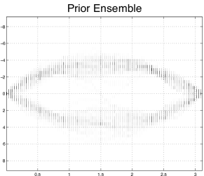
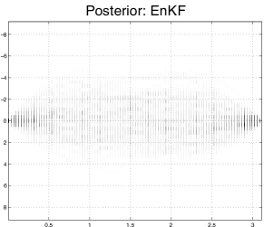
(a)	(b)
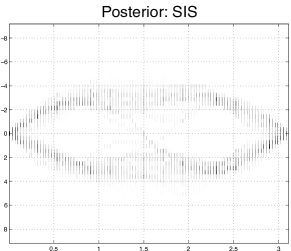
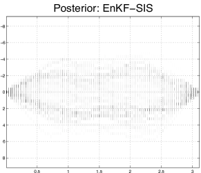
(c)	(d)

Figure 3: EnKF smears non-Gaussian distribution. The horizontal axis is the spatial coordinate $x\in[0,\pi]$. The vertical axis is the value of function $u$. The level of shading on each vertical line is the marginal density of $u$ at a fixed $x$, computed from a histogram with 50 bins. While EnKF completely ignores the non-Gaussian character of the posterior and centers the distribution around $u=0$, EnKF-SIS shows darker bands at the edges.

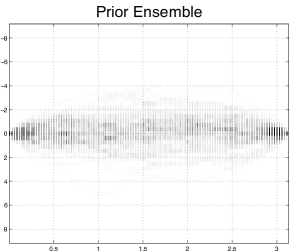
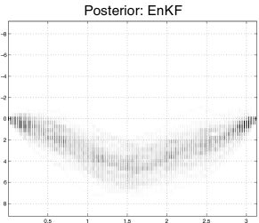
(a)	(b)
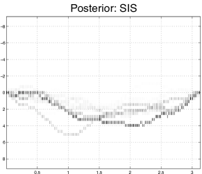
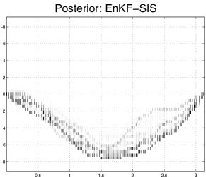
(c)	(d)

Figure 4: SIS cannot make a large update. The horizontal axis is the spatial coordinate $x\in[0,\pi]$. The vertical axis is the value of function $u$. The level of shading on each vertical line is the marginal density of $u$ at a fixed $x$, computed from a histogram with 50 bins. While EnKF and EnKF-SIS create ensembles that are attracted to the data value $u(\pi/2)=7$, SIS cannot reach so far because there are no such members in this relatively small ensemble of size $N=100$.

Finally, typical results for filtering in the space of functions on $[0,\pi]$ of the form

$$u=\sum_{n=1}^{d}c_{n}\sin\left(nx\right)$$ (6)

are in Figs. 3 and 4. The ensemble size was $N=100$ and the dimension of the state space was $d=500$. The Fourier coefficients were chosen $\lambda_{n}=n^{-3}$ to generate the initial ensemble from (1), and $\kappa_{n}=n^{-2}$ for the norm in the density estimation.

Fig. 3 again shows that EnKF cannot handle bimodal distribution. The prior was constructed by assimilating the data likelihood

$$p(d|u)=\left\{\begin{array}[c]{l}1/2\mbox{ if }u(\pi/4)\mbox{ and }\\ \quad\quad u\left(3\pi/4\right)\in\left(-2,-1\right)\cup(1,2)\\ 0\mbox{ otherwise}\end{array}\right.$$

into a large initial ensemble (size 50000) and resampling to the obtain the forecast ensemble size $N=100$ with a non-Gaussian density. Then the data likelihood $u\left(\pi/2\right)-0.1\sim N(0,1)$ was assimilated to obtain the analysis ensemble.

Fig. 4 shows a failure of SIS. The prior ensemble sampled from Gaussian distribution with coefficients $\lambda_{n}=n^{-3}$ using (1) and (6), and the data likelihood was $u\left(\pi/2\right)-7\sim N(0,1)$.

4 Conclusion

We have demonstrated the potential of a predictor-corrector filter to perform a successful Bayesian update in the presence of non-Gaussian distributions, large number of degrees of freedom, and large change of the state distribution. Open questions include convergence of the filter in high dimension when applied to multiple updates over time, mathematical convergence proofs for the density estimation and for the Bayesian update, and performance of the filters when applied to systems with a large number of different physical variables and modes, as is common in atmospheric models.

Acknowledgements.

This work was supported by the National Science Foundation under grants CNS-0719641, ATM-0835579, and CNS-0821794.

References

- [1] Darema, F.: Dynamic data driven applications systems: A new paradigm for application simulations and measurements. In: Bubak, M., van Albada, G.D., Sloot, P.M.A., Dongarra, J.J. (eds.) ICCS 2004, LNCS, vol. 3038, pp. 662–669. Springer (2004)
- [2] Kalnay, E.: Atmospheric Modeling, Data Assimilation and Predictability. Cambridge University Press (2003)
- [3] Burgers, G., van Leeuwen, P.J., and Evensen, G.: Analysis scheme in the ensemble Kalman filter. Monthly Weather Rev. 126 (1998) 1719–1724
- [4] Doucet, A., de Freitas, N., Gordon, N. (eds.) Sequential Monte Carlo in Practice. Springer (2001)
- [5] Evensen, G.: The ensemble Kalman filter: Theoretical formulation and practical implementation. Ocean Dynamics 53 (2003) 343–367
- [6] Anderson, J.L.: An ensemble adjustment Kalman filter for data assimilation. Monthly Weather Rev. 129 (1999) 2884–2903
- [7] Mitchell, H.L., Houtekamer, P.L.: An adaptive ensemble Kalman filter. Monthly Weather Rev. 128 (2000) 416–433
- [8] Bengtsson, T., Snyder, C., Nychka, D.: Toward a nonlinear ensemble filter for high dimensional systems. J. of Geophysical Research - Atmospheres 108(D24) (2003) STS 2–1–10
- [9] Mandel, J., Beezley, J.D.: Predictor-corrector ensemble filters for the assimilation of sparse data into high dimensional nonlinear systems. CCM Report 232, University of Colorado Denver (2006)
- [10] Mandel, J., Beezley, J.D.: Predictor-corrector and morphing ensemble filters for the assimilation of sparse data into high dimensional nonlinear systems. In: 11th Symposium on Integrated Observing and Assimilation Systems for the Atmosphere, Oceans, and Land Surface (IOAS-AOLS), CD-ROM, Paper 4.12, 87th American Meteorological Society Annual Meeting, San Antonio, TX, http://ams.confex.com/ams/87ANNUAL/techprogram/paper_119633.htm (2007)
- [11] Mandel, J., Beezley, J.D.: Predictor-corrector ensemble filters for data assimilation into high-dimensional nonlinear systems. In preparation (2009).
- [12] Evensen, G.: Sequential data assimilation with nonlinear quasi-geostrophic model using Monte Carlo methods to forecast error statistics. J. of Geophysical Research 99 (C5) (1994) 143–162
- [13] Loftsgaarden, D.O., Quesenberry, C.P.: A nonparametric estimate of a multivariate density function. Ann. Math. Stat. 36 (1965) 1049–1051
- [14] Kim, S., Eyink, G.L., Restrepo, J.M., Alexander, F.J., Johnson, G.: Ensemble filtering for nonlinear dynamics. Monthly Weather Rev. 131 (2003) 2586–2594
- [15] Miller, R.N., Carter, E.F., Blue, S.T.: Data assimilation into nonlinear stochastic models. Tellus 51A (1999) 167–194
- [16] Higham, D.J.: An algorithmic introduction to numerical simulation of stochastic differential equations. SIAM Rev. 43 (2001) 525–546