Possible duality violations in $\tau$ decay and their impact on the determination of $\alpha_{s}$

Oscar Catà,¹ Maarten Golterman,² and Santiago Peris³

¹INFN, Laboratori Nazionali di Frascati, Via E. Fermi 40, I-00044 Frascati, Italy

²Department of Physics and Astronomy, San Francisco State University,

1600 Holloway Ave, San Francisco, CA 94132, USA

³Grup de Física Teòrica and IFAE, UAB, E-08193 Bellaterra, Barcelona, Spain

We discuss the issue of duality violations in hadronic tau decay. After introducing a physically motivated ansatz for duality violations, we estimate their possible size by fitting this ansatz to the tau experimental data provided by the ALEPH collaboration. Our conclusion is that these data do not exclude significant duality violations in tau decay. This may imply an additional systematic error in the value of $\alpha_{s}(m_{\tau})$, extracted from tau decay, as large as $\delta\alpha_{s}(m_{\tau})\sim 0.003-0.010$ .

1 Introduction

The hadronic decay of the tau lepton is a particularly suitable process for studying QCD interactions, because its mass is heavy enough to produce hadrons in the final state, without the complications which arise with hadrons in the initial state. However, since the mass of the tau is not much larger than a typical hadronic scale of order $1$ GeV, it was initially unclear whether a perturbative QCD analysis of this process would not be ruined by nonperturbative effects beyond any systematic control. The pioneering work of Ref. [1] showed, however, that perturbation theory, augmented with the Operator Product Expansion (OPE) [2], can indeed be the right tool for understanding strong interaction aspects of hadronic tau decay. Among these, the most important ones are perhaps the determination of the coupling constant $\alpha_{s}$, the light quark masses, and the vacuum condensates [3].

In fact, the determination of $\alpha_{s}$ from tau decay is now one of the most accurate ones. The level of accuracy is so high that subtle effects, which were completely negligible before, may now start to play a significant role in the precision of the result. Since the value of $\alpha_{s}$ is of fundamental importance for our understanding of QCD and the Standard Model, it is obvious that a good control of all systematic effects is, now more than ever, mandatory.

References [5, 6, 7, 8] find the following values for $\alpha_{s}$ after analyzing the same experimental data obtained by ALEPH [4]:

$$\alpha_{s}(m_{\tau}^{2}) = 0.344\pm 0.005_{\mathrm{exp}}\pm 0.007_{\mathrm{th}}\quad\cite[cite]{[\@@bibref{}{Davier}{}{}]}\ ,$$

$$\alpha_{s}(m_{\tau}^{2}) = 0.332\pm 0.005_{\mathrm{exp}}\pm 0.015_{\mathrm{th}}\quad\cite[cite]{[\@@bibref{}{Baikov}{}{}]}\ ,$$

$$\alpha_{s}(m_{\tau}^{2}) = 0.321\pm 0.005_{\mathrm{exp}}\pm 0.012_{\mathrm{th}}\quad\cite[cite]{[\@@bibref{}{Maltman}{}{}]}\ ,$$

$$\alpha_{s}(m_{\tau}^{2}) = 0.316\pm 0.003_{\mathrm{exp}}\pm 0.005_{\mathrm{th}}\quad\cite[cite]{[\@@bibref{}{Jamin}{}{}]}\ .$$ (1.1)

Note that, if the errors are taken at face value, these four results are not fully consistent with one another. The main difference between the results of Refs. [5] and [8] is due to the treatment of perturbation theory (the use of so-called Contour-Improved (CI) vs Fixed-Order (FO) resummation prescriptions, respectively [9]). This difference has been included in the systematic error in [6]. The difference between the result of Ref. [7] and the other three is mainly due to the use of different weight functions in the finite-energy sum rules. Different choices for these functions distribute differently the relative weight between the perturbative and the OPE contributions, as extracted from the spectral function. Although in an exact treatment these choices should not matter, in practice they do since truncations of both the perturbative series and higher orders in the OPE have to be applied. Ref. [7] also analyzes the effect of some of these higher orders in the OPE.

Another interesting “mismatch” is seen in the analysis of the ALEPH data carried out in Ref. [5], which quotes the following values for the gluon condensate:

$$\frac{\alpha_{s}}{\pi}\langle GG\rangle\Big{|}_{\mathrm{Vector}}\!\! = (-0.8\pm 0.4)\times 10^{-2}\ {\mathrm{GeV}}^{4}\ ,$$ (1.2)

$$\frac{\alpha_{s}}{\pi}\langle GG\rangle\Big{|}_{\mathrm{Axial}} = (-2.2\pm 0.4)\times 10^{-2}\ {\mathrm{GeV}}^{4}\ ,$$

where the subscript denotes whether the condensate has been determined using the vector or the axial-vector spectral function. Although these two quantities should be one and the same in QCD, it is clear that the two values in Eq. (1.2) are not compatible with each other. Of course, the discrepancies (1) and (1.2) would not be there if either a) one could argue that a specific analysis is to be preferred on theoretical grounds, or b) if the errors had been underestimated because of yet other systematic effects. Further determinations of the OPE condensates may be found in Refs. [10].

From the theoretical point of view, one could think of (at least) three sources of possible systematic errors, namely the truncation of the perturbative series in powers of $\alpha_{s}$, the truncation of the OPE, and the contribution from Duality Violations (DVs). In fact, at some deeper level, the three sources must be related. First, the purely perturbative contributions can be viewed as the contribution from the dimension-zero “condensate” (i.e., the unit operator) to the OPE. Second, the lack of convergence of the perturbative series in $\alpha_{s}$ calls for the existence of some nonperturbative contribution which, through renormalons, is related to the OPE condensates. Finally, the lack of convergence of the OPE is, in turn, at the origin of DVs.

It is far from clear that the different values for $\alpha_{s}$ quoted in Eqs. (1) should be due to DVs, since the first two error sources mentioned above can potentially explain this difference by themselves. However, in this work we will concentrate on DVs as a further possible source of error, because it has been much less explored than the other two.

In QCD analyses of tau decays, the OPE plays a central role. However, although this expansion is of such fundamental importance, the properties of the OPE in QCD are not known. In particular, although it is suspected that the OPE is asymptotic, this is not known to be true, and, even if it is indeed asymptotic, we do not know whether it is summable or not, or how it behaves along different rays in the $q^{2}$ complex plane. For an asymptotic expansion, it is of course important to estimate its intrinsic theoretical error. Relegating a more precise definition of this error to the discussion in the next section, here we just mention that this intrinsic theoretical error is normally associated with DVs.

In practice, one can perhaps get a feeling of the systematic error in the perturbative expansion by comparing different orders in the $\alpha_{s}$ expansion. Likewise, the systematic error in the condensate contribution may also be assessed from the comparison between different orders in the OPE. However, we do not know of any systematic approach for studying DVs. Therefore, although the disagreement between, e.g., the results quoted in Eq. (1.2) may point towards the fact that “this method may approach its ultimate accuracy” in tau decay [5], there is currently no method to estimate this accuracy from first principles in QCD. Hence, there appears to be no other way to make progress than to resort to models.

Based on tau data, the only attempt to date at estimating the error from DVs is the one made in Ref. [5]; their claim is that DVs effects are completely negligible at the tau mass. This result was obtained from the V+A spectral function with the help of a physically motivated model, previously used for studying aspects of DVs [14, 15, 16, 17]. In the present work, we reanalyze this estimate studying separately the V and A correlators. As we will see, our conclusion is different: based on tau data alone, DVs may be larger than those found in Ref. [5]. The inclusion of $e^{+}e^{-}$ data beyond the $\tau$ mass, with some extra assumptions to be detailed below, may also be used to further constrain the size of DVs but, even in this case, their impact could be comparable to the presently quoted systematic uncertainties. Therefore, the possible effect of DVs should be taken into account.

This work is organized as follows. In Section 2, we present the theoretical background needed for the discussion of DVs in tau decay, while in Section 3 we introduce and motivate our ansatz for DVs. The actual fits to the experimental tau data are described in Section 4. Section 5 is devoted to an estimate of the impact of these fits on the determination of $\alpha_{s}$ and, in Section 6, we assess the changes imposed on this estimate if one also considers recent $e^{+}e^{-}$ data beyond the $\tau$ mass. Finally, in Section 7, we offer some conclusions and prospects for future work.

2 Duality violations and $\tau$ decay

Let us start our discussion of hadronic tau decay by defining the correlators

$$\Pi^{V,A}_{\mu\nu}(q) = i\int\mathrm{d}^{4}x\,e^{iq\cdot x}\langle\,0\,|\,T\{\,J_{\mu}(x)\,J_{\nu}^{\dagger}(0)\,\}|\,0\,\rangle\,$$ (2.1)

$$= (q^{\mu}q^{\nu}-q^{2}g^{\mu\nu})\,{\mathrm{Im}}\,\Pi_{V,A}^{(1)}(s)+q^{\mu}q^{\nu}\,\Pi_{V,A}^{(0)}(q^{2})\ ,$$

in which $J_{\mu}^{V}(x)=\bar{u}(x)\gamma_{\mu}d(x)$ and $J_{\mu}^{A}(x)=\bar{u}(x)\gamma_{\mu}\gamma_{5}d(x)$. The ratio of the decay widths of the tau lepton to nonstrange (vector and axial-vector channel) hadrons and the decay width to electrons, denoted as

$$R_{\tau}^{V,A}\equiv\frac{\Gamma[\tau^{-}\rightarrow(V^{-},A^{-})\nu_{\tau}]}{\Gamma[\tau^{-}\rightarrow\nu_{\tau}e^{-}{\bar{\nu}}_{e}]}\ ,$$ (2.2)

can be expressed as

$$R_{\tau}^{V,A}\!\!=12\pi S_{EW}|V_{ud}|^{2}\!\!\!\int_{0}^{m_{\tau}^{2}}\!\!\frac{ds}{m_{\tau}^{2}}\left(1-\frac{s}{m_{\tau}^{2}}\right)^{2}\left[\left(1+2\frac{s}{m_{\tau}^{2}}\right){\mathrm{Im}}\,\Pi_{V,A}^{(1)}(s)+{\mathrm{Im}}\,\Pi_{V,A}^{(0)}(s)\right]\ ,$$ (2.3)

where the factor $S_{EW}=1.0201(3)$ [11] accounts for small, known electroweak corrections, and $V_{ud}$ is the corresponding entry in the CKM matrix.

Figure 1: Analytic structure of $\Pi_{V,A}(q^{2})$ in the complex $q^{2}$ plane. The solid curve shows the contour used in Eq. (2.4).

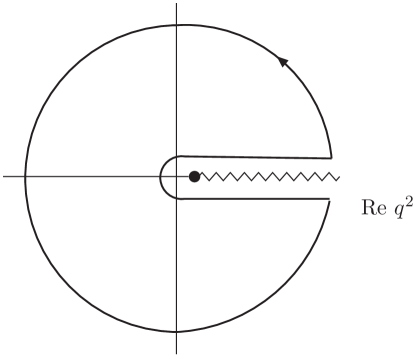
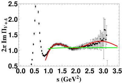
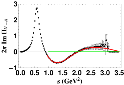
The spectral functions ${\mathrm{Im}}\,\Pi_{V,A}^{(1)}(s)$ appearing in Eq. (2.3) have been measured most accurately by ALEPH [4], and the results are included in Fig. 3 below. Since at present these spectral functions cannot be directly calculated from QCD, what is being done in practice, following Refs. [1, 12, 13], is to take advantage of the analytic properties of the functions $\Pi_{V,A}^{(1)}(q^{2})$ in the complex $q^{2}$ plane, depicted in Fig. 1. We write (dropping the superscript ⁽¹⁾ from now on)

$$\int_{0}^{s_{0}}\,ds\,\,P(s)\,\frac{1}{\pi}{\mathrm{Im}}\,\Pi_{V,A}(s)=-\frac{1}{2\pi i}\oint_{|q^{2}|=s_{0}}\,dq^{2}\,P(q^{2})\,\Pi_{V,A}(q^{2})\ ,$$ (2.4)

where $P(q^{2})$ is an arbitrary polynomial which can be chosen at one’s convenience. In the application to tau decay one sets the radius $s_{0}=m_{\tau}^{2}$ and, under the assumption that this scale is larger than the scale at which the OPE sets in, it makes sense to rewrite the right hand side of Eq. (2.4) as

$$-\frac{1}{2\pi i}\oint_{|q^{2}|=s_{0}}\,dq^{2}\,P(q^{2})\,\Big{\{}\Pi^{\mathrm{OPE}}_{V,A}(q^{2})+\Delta_{V,A}(q^{2})\Big{\}}\ ,$$ (2.5)

where, by definition,

$$\Delta_{V,A}(q^{2})=\Pi_{V,A}(q^{2})-\Pi^{\mathrm{OPE}}_{V,A}(q^{2})\ ,$$ (2.6)

and then approximate $\Delta_{V,A}(q^{2})\sim 0$, thus neglecting the second term in Eq. (2.5). To the best of our knowledge, in all analyses of tau decay to date, except for Ref. [5], this approximation has always been assumed. As we already mentioned in the introduction, Ref. [5] does discuss the possibility of DVs in tau decay, but only for the combined V+A correlator, and concludes that DVs are negligible and do not affect the systematic errors from other sources, cf. the first result quoted in Eq. (1).

Here we will not assume this approximation. On the contrary, we will take nonvanishing contributions to $\Delta_{V,A}(q^{2})$ as defined in Eq. (2.6) as the definition of DVs. Consequently, if we define

$${\cal{D}}_{V,A}^{[P]}(s_{0})=-\frac{1}{2\pi i}\oint_{|q^{2}|=s_{0}}\,dq^{2}\,P(q^{2})\,\Delta_{V,A}(q^{2})\ ,$$ (2.7)

as a measure of these DVs in tau decay, Eq. (2.4) becomes

$$\int_{0}^{s_{0}}\,ds\,\,P(s)\,\frac{1}{\pi}{\mathrm{Im}}\,\Pi_{V,A}(s)=-\frac{1}{2\pi i}\oint_{|q^{2}|=s_{0}}\,dq^{2}\,P(q^{2})\,\Pi^{OPE}_{V,A}(q^{2})+{\cal{D}}_{V,A}^{[P]}(s_{0})\ .$$ (2.8)

Note that, if the OPE were a convergent expansion and $s_{0}$ were within the radius of convergence, one would get $\Delta_{V,A}(q^{2})=0$ and thus DVs would be absent.

Although the precise convergence properties of the OPE in the complex plane are not known, we do know that this power expansion cannot be convergent but only asymptotic (at best). A convergent expansion around $|q^{2}|=\infty$ in the complex plane defines an analytic function on a complete annulus around the origin, which must, therefore, also include the Minkowski axis. However, this is contradicted by the existence of the physical cut along the Minkowski axis, which shows that the expansion cannot be convergent for any $s_{0}$.

In this work we will assume that the OPE is an asymptotic expansion in $q^{2}$ and explore the possible consequences. As an asymptotic expansion, the OPE will have a region of validity (the so-called wedge of asymptoticity [18]) which will naturally exclude the Minkowski axis. This expectation is strongly supported by the large-$N_{c}$ limit, for which the physical cut becomes an infinite set of poles which are not reproduced by the OPE. We remark that, even if the function $P(q^{2})$ is chosen such that it vanishes on the Minkowski axis (as is the case for the polynomial appearing in the integrand of Eq. (2.3)), that does not guarantee that the DV function ${\cal{D}}_{V,A}^{[P]}(s_{0})$ will exactly vanish.

Figure 2: Contour used in the derivation of Eq. (2.9). With the assumed exponential decay, $\Delta_{V,A}(q^{2})$ vanish on the dashed circle with infinite radius.

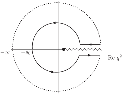
Accepting that the OPE is asymptotic, it is natural to assume a momentum dependence of the DV function $\Delta_{V,A}(q^{2})$ with an exponential decay at large $|q^{2}|$. Then, using the contour depicted in Fig. 2 and the exponential decay of $\Delta_{V,A}(q^{2})$ on the dashed circle at infinity, one obtains a simpler expression for ${\cal{D}}_{V,A}^{[P]}(s_{0})$ [16, 17]:

$${\cal{D}}_{V,A}^{[P]}(s_{0})=-\int_{s_{0}}^{\infty}ds\ P(s)\ \frac{1}{\pi}\mathrm{Im}\Delta_{V,A}(s)\ .$$ (2.9)

This relation is interesting for two reasons. It is useful, since it expresses the DV contribution to Eq. (2.8), ${\cal{D}}_{V,A}^{[P]}(s_{0})$, as an integral along the Minkowski axis, in terms of the spectral function, and it can thus in principle be determined from experimental data (as we will do below). However, this requires an extrapolation from values of $s$ for which experimental data are available to infinity. This shows explicitly the inherent difficulty present in any quantitative evaluation of DVs [19].

3 An ansatz for Duality Violations

To make progress one clearly needs information about the functions $\mathrm{Im}\Delta_{V,A}(s)$. However, as emphasized above, it is not known how to get this information from QCD. Therefore, there is no other option but to adopt an ansatz which is theoretically sensible and which is, of course, not ruled out by existing data. In other words, we look for a consistent picture of how duality violations might occur in QCD, and how they may affect the existing determinations of $\alpha_{s}$ (and, consequently, also quark masses and condensates). This way we are able to make an educated guess about the possible size of the systematic errors due to DVs as allowed by existing data.

We will parametrize the duality-violating part of the spectral functions as

$$\frac{1}{\pi}\mathrm{Im}\Delta_{V,A}(s)=\kappa_{V,A}\ e^{-\gamma_{V,A}s}\ \sin\left(\alpha_{V,A}+\beta_{V,A}s\right)\ ,$$ (3.1)

The exponential decay in this expression is inspired by our assumption that the OPE is an asymptotic expansion, and can be understood as representing the finite width of resonances [14]. The oscillatory behavior is what one expects in a spectral function with resonances exhibiting some kind of periodicity. The precise form chosen here is that obtained if the vector and axial-vector resonances lie on Regge daughter trajectories.

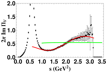
Furthermore, a glance at Fig. 3 reveals that both the vector and the axial-vector spectral functions cross perturbation theory around $s=2$ GeV². A natural interpretation is that the corresponding DV functions $\mathrm{Im}\Delta_{V,A}(q^{2})$ have a zero near this energy. Such a zero is much harder to understand without DVs since, in this case, it would have to be due to a cancelation between different orders of the OPE, signalling a possible breakdown of the OPE. Although we cannot exclude such a breakdown at this rather high scale for minkowskian momentum, much evidence is consistent with the OPE being valid to a significantly lower scale for euclidean momentum, whether this scale is associated with the gluon condensate or with the quark condensate. Such a hypothetical breakdown is also not seen in the purely perturbative contribution, which remains small and essentially flat all the way down to 1 GeV². Furthermore, as we will see in the next section and the Appendix, the OPE yields very small contributions to the $V$ and $A$ spectral functions from the condensates of dimension four and six down to $1$ GeV².

Figure 3: Different combinations of spectral functions ($V$, $A$, and $V\pm A$) (data points in black) compared with fixed-order perturbation theory (green flat line) and the result of our fit to Eq. (3.1), (red curve).

Since the width of a resonance is a $1/N_{c}$ effect, one expects the exponent $\gamma$ to be relatively small. The reason is that it has to go to zero when $N_{c}$ goes to infinity, since the exponential suppression shown in Eq. (3.1) has to disappear in favor of an unsuppressed contribution representing the isolated, infinitely narrow peaks present in any spectral function in QCD in the strict $N_{c}\rightarrow\infty$ limit. For the other parameters we expect $\kappa$ to be of order $N_{c}$, and $\alpha$ and $\beta$ are expected to be of order one in this limit.

Although our arguments are admittedly rather heuristic, it is reassuring that a mathematical model realizing all the above features actually exists. In this model, first proposed in Refs. [14, 15], resonance widths are introduced in a manner compatible with the analytic properties of the correlators (2.1), with masses following Regge theory. This model is physically well motivated, and has been used for a variety of studies of DVs for both light and heavy quarks [15, 16, 17, 5]. Our ansatz, Eq. (3.1), actually corresponds to the asymptotic behavior of this mathematical model for large $s$. By considering the approximation (3.1) with a priori unknown values for the parameters $\alpha,\beta,\gamma$ and $\kappa$, we expect to describe the generic features of DVs at large $s$, avoiding some of the more model-dependent details. We note, however, that the ansatz (3.1) is a very good approximation to the full mathematical model already at relatively low values of $s$ [16].

4 Fit to tau data

To find out whether the ansatz (3.1) is compatible with the tau experimental data, we have fitted the ALEPH spectral functions in both the vector and axial-vector channels, i.e., we fitted the spectral data with the functions

$$\frac{1}{\pi}\mathrm{Im}\Pi_{V,A}(s)=\theta(s-s_{min})\ \left\{\frac{N_{c}}{12\pi^{2}}\big{[}1+\widehat{\rho}(s)\big{]}+\kappa_{V,A}\ e^{-\gamma_{V,A}s}\ \sin\big{(}\alpha_{V,A}+\beta_{V,A}s\big{)}\right\}\ .$$ (4.1)

The function $\widehat{\rho}(s)$ above contains the purely perturbative corrections in powers of $\alpha_{s}$ up to ${\cal{O}}(\alpha_{s}^{5})$. These perturbative corrections differ depending on whether one uses CI or FO perturbation theory and the expressions for both treatments have been taken from Ref. [8], where one can also find a discussion of their relevance for tau decay.

In principle one should also include in Eq. (4.1) the contribution from the condensates which, away from $q^{2}=0$, can only come from the logarithms in the Wilson coefficients. However, the contribution from the operators of dimension four and six turns out to be numerically very small for reasonable values of the quark and gluon condensates. Our estimates for these contributions are relegated to the Appendix. Condensates of dimension eight or higher will not be considered.

As already mentioned in the previous section, the ansatz (3.1) is to be understood as an estimate of DVs at large values of $s$. Since, in practice, we do not know how large $s$ would have to be, we have done our fits in a window $s_{min}\leq s\leq m_{\tau}^{2}$, varying the lower end, $s_{min}$. In other words, in the phenomenological approach we will be taking, the precise meaning of large values of $s$ will be set by the quality of the fit. The results of the fit are very insensitive to the value of $s_{min}$, between a maximum value of $s_{min}$ of $\sim 1.8$ GeV² (above this value the experimental errors are too large for the fit to be meaningful), and a minimum value of $s_{min}$ of $\sim 1.1$ GeV². Below this value there is a sharp increase in the chi-squared per degree of freedom, showing a deterioration of the fit, probably due to the tail of the $\rho$ meson (in the vector channel). Consequently, we have chosen $1.1$ GeV${}^{2}\leq s\leq m_{\tau}^{2}$ as our fitting window.

The result of the fit to the vector spectral function is then:

$$\kappa_{V} = 0.018\pm 0.004\ ,$$

$$\gamma_{V} = 0.15\pm 0.15\ \mathrm{GeV}^{-2}\ ,$$

$$\alpha_{V} = 2.2\pm 0.3\ ,$$

$$\beta_{V} = 2.0\pm 0.1\ \mathrm{GeV}^{-2}\ ,$$

$$\frac{\chi^{2}}{dof} = \frac{10}{79}\simeq 0.13\quad,$$ (4.2)

and that to the axial-vector spectrum:

$$\kappa_{A} = \ 0.20\pm 0.06\ ,$$

$$\gamma_{A} = \ 1.7\pm 0.2\ \mathrm{GeV}^{-2}\ ,$$

$$\alpha_{A} = -0.4\pm 0.1\ ,$$

$$\beta_{A} = -3.0\pm 0.1\ \mathrm{GeV}^{-2}\ ,$$

$$\frac{\chi^{2}}{dof} = \frac{17}{78}\simeq 0.22\quad.$$ (4.3)

Even though the perturbative term $\widehat{\rho}(s)$ in Eq. (4.1) is different in the CI or FO resummation schemes, the results for the fit parameters are, within the quoted errors, insensitive to this difference, or to the initial value for $\alpha_{s}$, which we took to be $\alpha_{s}(m_{\tau})=0.3156$. Our fits are also rather insensitive to an increase of the value of $s_{min}$; the main effect is an increase of the errors quoted in Eqs. (4,4).

Since our lower end is at $s=1.1$ GeV², one may worry about the use of perturbation theory at such low scales. However, there is nothing in the perturbative expansion signalling a breakdown of the approximation, as the nearly horizontal line in Fig. 3 clearly shows. Also, one may object that perturbation theory and the OPE should not be used for describing a spectral function on the time-like axis, Eq. (4.1), i.e., that “local duality” does not work. However, we want to emphasize that local duality does not work precisely because DVs are not included, and that DVs, parametrized for example as in Eq. (4.1), amount to adding the necessary contributions which make up for the missing piece, therefore making local duality exact (cf. Eq. (2.8)). Our analysis thus amounts to the assumption that Eq. (4.1) gives a reasonable account of DVs above $s=s_{min}$.

Looking at the values obtained from the fits (4,4), one immediately realizes that the oscillations in the axial-vector channel will be more damped than in the vector channel as a result of a much larger exponent, i.e., $\gamma_{A}\gg\gamma_{V}$. While we have no understanding of why this should be so in QCD, we simply observe that the difference in the values of these parameters reflects the difference in the corresponding spectra as measured by ALEPH.

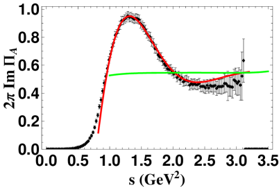
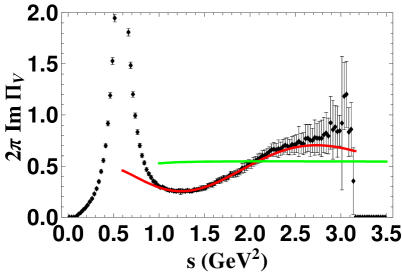
Fig. 3 shows the comparison of the fits to the different combinations of experimental spectral functions. As one can see, all fits are very good, having a very small $\chi^{2}/dof$. Our fits are fully correlated fits, i.e., correlations among errors were taken into account in both fits using the pertinent covariance matrix provided by ALEPH. The small values of $\chi^{2}/dof$ that we find might suggest an underestimation of these correlations (or an overestimate of the diagonal errors), although it is difficult to know whether this is actually the case. In fact, an uncorrelated fit using only the diagonal entries of the covariance matrices leads to results which are similar to those in Eq. (4,4), in particular for the vector spectral function. We remark that our analysis is not the only one to get such small values for $\chi^{2}/dof$. The analysis of Ref. [5] finds a value of $\chi^{2}/dof=0.07$ in their OPE fit to moments such as Eq. (2.3) in the vector channel.

As can be seen from Fig. 3, the vector and axial-vector spectral functions oscillate around perturbation theory in the window 1 GeV${}^{2}\leq s\leq m_{\tau}^{2}$ with almost complete anti-correlation, with a common“oscillation node” around 2 GeV². Therefore the combination $V+A$ agrees with perturbation theory better than $V$ or $A$ individually. Furthermore, the fits of Refs. [1, 5] suggest that there is a partial cancelation in the $V+A$ combination of the contribution to the contour integral in Eq. (2.5) from both the dimension-six and dimension-eight condensates in the OPE. These features have led people to believe that the combination $V+A$ is a better correlation function than $V$ or $A$, because it is somehow protected from all kinds of nonperturbative effects, including DVs. However, as the third panel on Fig. 3 shows, the partial agreement of perturbation theory (green flat line) with the experimental $V+A$ data does not guarantee the absence of DVs. In fact, the results of our fits reported in Eqs. (4,4) reproduce the experimental data better than perturbation theory and, consequently, constitute a clear indication that nonzero DVs may exist in this spectral function as well. Furthermore, because DVs are suppressed in the axial-vector channel due to the large exponent $\gamma_{A}$, the amount of DVs in $V+A$ is basically the same as in $V$. In our opinion, this example shows that one should understand the $V$ and $A$ channels individually before drawing any definite conclusion about $V+A$.

5 Impact of Duality Violations on $R_{\tau}$ and $\alpha_{s}$

Once the DV functions (3.1), along with the values for the parameters (4,4), are known, one can use Eq. (2.8) to calculate the contribution from our DV ansatz to $R_{\tau}$. This is given by

$$R_{\tau}^{V,A} = (R_{\tau}^{V,A})^{(0)}-12\pi S_{EW}|V_{ud}|^{2}\int^{\infty}_{m_{\tau}^{2}}\frac{ds}{m_{\tau}^{2}}\left(1-\frac{s}{m_{\tau}^{2}}\right)^{2}\left(1+2\frac{s}{m_{\tau}^{2}}\right){\mathrm{Im}}\,\Delta_{V,A}(s)$$ (5.1)

$$\equiv (R_{\tau}^{V,A})^{(0)}+\delta R_{\tau}^{V,A}\ ,$$

where $(R_{\tau}^{V,A})^{(0)}$ corresponds to the case of no DVs and, consequently, $\delta R_{\tau}^{V,A}$ corresponds to the contribution from duality violations. In the case of our ansatz (3.1), we obtain

$$\delta R_{\tau}^{V,A} = -\ \frac{72\pi^{2}\kappa_{V,A}\ e^{-\gamma_{V,A}m_{\tau}^{2}}}{(\beta_{V,A}^{2}+\gamma_{V,A}^{2})^{4}\ m_{\tau}^{8}}S_{EW}|V_{ud}|^{2}$$ (5.2)

$$\Big{\{}\Phi_{1}(m_{\tau}^{2})\ \sin{\left(\alpha_{V,A}+\beta_{V,A}m_{\tau}^{2}\right)}+\Phi_{2}(m_{\tau}^{2})\ \cos{\left(\alpha_{V,A}+\beta_{V,A}m_{\tau}^{2}\right)}\Big{\}}\ ,$$

with

$$\Phi_{1}(m_{\tau}^{2}) = 2\beta_{V,A}^{4}-12\gamma_{V,A}^{2}\beta_{V,A}^{2}+2\gamma_{V,A}^{4}-\Big{(}3\gamma_{V,A}\beta_{V,A}^{4}+2\gamma_{V,A}^{3}\beta_{V,A}^{2}-\gamma_{V,A}^{5}\Big{)}m_{\tau}^{2}\ ,$$

$$\Phi_{2}(m_{\tau}^{2}) = 8\gamma_{V,A}\beta_{V,A}(\gamma_{V,A}^{2}-\beta_{V,A}^{2})-\Big{(}\beta_{V,A}^{5}-2\gamma_{V,A}^{2}\beta_{V,A}^{3}-3\gamma_{V,A}^{4}\beta_{V,A}\Big{)}m_{\tau}^{2}\ ,$$ (5.3)

for $s_{0}=m_{\tau}^{2}$. Note that $\delta R_{\tau}^{V,A}$ goes to zero for $\gamma_{V,A}\rightarrow\infty$, but is finite in the $\gamma_{V,A}\rightarrow 0$ limit. Upon substituting the values from the vector and axial-vector fits (4,4) one finds

$$\delta R_{\tau}^{V}=\left(-0.022\pm 0.013\right)\ S_{EW}|V_{ud}|^{2}\ ;\ \delta R_{\tau}^{A}=\left(0.0003\pm 0.0003\right)\ S_{EW}|V_{ud}|^{2}\ ,$$ (5.4)

which translates into $\delta R_{\tau}^{V}/R_{\tau}^{V}\simeq-(1.5\pm 0.9)\%$ and $\delta R_{\tau}^{A}/R_{\tau}^{A}\simeq(0.02\pm 0.02)\%$. The effect of DVs is much smaller in the axial-vector channel, because of the larger $\gamma_{A}$, as anticipated.

For comparison, Ref. [5] takes the resonance model in Ref. [14] as a model for DVs, matches it directly to the $V+A$ spectral function near $s=m^{2}_{\tau}$, and finds that the effect of DVs is at most $\delta R_{\tau}^{V+A}\simeq 0.0021S_{EW}|V_{ud}|^{2}$. In our case we keep only the form of the asymptotic behavior of this type of model for the spectral function (cf. Eq. (3.1)), and we then fit the parameters of this ansatz to the $V$ and $A$ spectral functions separately. We thus find for the effect in $V+A$ the sum of the two results in Eq. (5.4), which is ten times larger than the estimate of Ref. [5], but still consistent with the experimental data. Ref. [5] also considers an instanton-based model [14]. In this case, the model does not have the exponential suppression of Eq. (3.1), and the contribution becomes $\delta R_{\tau}^{V+A}\simeq 0.014S_{EW}|V_{ud}|^{2}$. As it turns out, this is closer to our estimate in magnitude, although opposite in sign.

In order to estimate the shift in $\alpha_{s}$ induced by these values for $\delta R_{\tau}^{V,A}$, we first note that the perturbative expression for $R_{\tau}^{V+A}$ can be written as

$$(R_{\tau}^{V+A})_{PT}=\ N_{c}\ S_{EW}|V_{ud}|^{2}\left[1+\delta_{PT}\right]\ ,$$ (5.5)

with $\delta_{PT}$ given by the following expansions [8]

$$\delta_{PT}^{FO} = 0.1082\left(\frac{\alpha_{s}(m_{\tau})}{0.34}\right)+0.0609\left(\frac{\alpha_{s}(m_{\tau})}{0.34}\right)^{2}+$$ (5.6)

$$0.0334\left(\frac{\alpha_{s}(m_{\tau})}{0.34}\right)^{3}+0.0174\left(\frac{\alpha_{s}(m_{\tau})}{0.34}\right)^{4}+0.0088\left(\frac{\alpha_{s}(m_{\tau})}{0.34}\right)^{5}\ ,$$

$$\delta_{PT}^{CI} = 0.1479\left(\frac{\alpha_{s}(m_{\tau})}{0.34}\right)+0.0297\left(\frac{\alpha_{s}(m_{\tau})}{0.34}\right)^{2}+$$ (5.7)

$$0.0122\left(\frac{\alpha_{s}(m_{\tau})}{0.34}\right)^{3}+0.0086\left(\frac{\alpha_{s}(m_{\tau})}{0.34}\right)^{4}+0.0038\left(\frac{\alpha_{s}(m_{\tau})}{0.34}\right)^{5},$$

depending on whether one uses the CI or FO prescription. Using the experimental value for the tau decay ratio $R_{\tau}^{V+A}$ plus a conservative estimate for the main contributions from the condensates, Ref. [8] estimates the phenomenological value for the parameter $\delta$ as

$$\delta_{phen}=0.2042\pm 0.0050\ .$$ (5.8)

Equating $1+\delta_{PT}+\delta R_{\tau,V+A}/R_{\tau,V+A}$ to $1+\delta_{phen}$, one obtains an estimate for the shift in $\alpha_{s}$ due to the DV contribution (5.2), yielding

$$\delta\alpha_{s}(m_{\tau})\sim 0.003-0.010\ ,$$ (5.9)

both for CI and FO prescriptions. The spread of values in Eq. (5.9) reflects the error in the sum of the $V$ and $A$ results in Eq. (5.4), i.e., in $\delta R_{\tau}^{V+A}$.

We consider our result, Eq. (5.9), as a fair estimate of the systematic error associated with duality violations in $\alpha_{s}(m_{\tau})$, as determined from the total nonstrange tau decay width. However, the value of $\alpha_{s}(m_{\tau})$ and the condensates may also be determined from a combined fit to a set of moments written in terms of pinched weights (see, e.g., [5, 7]). In this case, our estimate is probably not good enough and a full analysis of these moments in the presence of DVs is required, for instance along the lines of our recently proposed iterative method described in Ref. [16]. At any rate, it is clear that the error associated with DVs is not numerically negligible, at least in the vector channel.

6 Inclusion of $e^{+}e^{-}$ data

Since, according to Eq. (2.9), DVs entail an extrapolation to high energies and, with our ansatz, they turn out to be sizeable in the vector channel, it makes sense to ask whether $e^{+}e^{-}$ data, which extend to higher energies than tau data, can be used to further restrict the range of values for the DV parameters (4).

However, one cannot relate DVs in tau decay to those in $e^{+}e^{-}$ without further assumptions. Since tau data concerns currents with a flavor structure of the type $\overline{u}d$, whereas $e^{+}e^{-}$ data see the flavor-singlet combination $(2/3)\overline{u}u-(1/3)\overline{d}d-(1/3)\overline{s}s$, there is an OZI suppressed contribution in $e^{+}e^{-}$ which is absent in tau decay. Although this contribution is $1/N_{c}$ suppressed and, in perturbation theory, shows up only at $\mathcal{O}(\alpha_{s}^{3})$, it is not clear how much it might affect the value of the DV parameters appearing in Eq. (3.1), since they encode nonperturbative effects on the time-like axis. As an exploratory step, we will simply assume that OZI contributions do not significantly affect the values of the parameters in the DV function (3.1). This is not the only difficulty, however. The strange quark mass is much larger than the up and down masses, and this should affect the values of the DV parameters for the $\overline{s}s$ component. Fortunately, taking guidance from the model underlying the form of our ansatz [14, 15, 16, 17], one finds that, while the parameters $\kappa_{V},\gamma_{V}$ and $\beta_{V}$ are related to the universal slope of the daughter Regge trajectories, the value of $\alpha_{V}$ is related to the mass (squared) of the lowest lying resonance of the Regge tower. This suggests that, while the value of $\alpha_{V}$ should be similar in the $\overline{u}u$ , $\overline{d}d$ and $\overline{u}d$ channels (assuming isospin symmetry), in the $\overline{s}s$ channel it should be shifted by a certain amount proportional to the strange quark mass. Since we do not know how large this shift may be, in practice we introduce a new parameter $\alpha^{\prime}_{V}$ for the $\overline{s}s$ component.

Figure 4: Plots of the vector spectral function in tau decay (left panel) and $e^{+}e^{-}$ (right panel) as compared to perturbation theory (green flat line) and the result of the combined fit (6) (red oscillating curve).

Therefore, in the context of $e^{+}e^{-}$ data, the spectral function including the ansatz for DVs becomes

$$\frac{1}{\pi}\mathrm{Im}\Pi_{V}(s) = \frac{N_{c}}{12\pi^{2}}\left[1+\widehat{\rho}(s)\right]+$$ (6.1)

$$\frac{5}{6}\ \kappa_{V}\ e^{-\gamma_{V}s}\ \sin\left(\alpha_{V}+\beta_{V}s\right)+\frac{1}{6}\ \kappa_{V}\ e^{-\gamma_{V}s}\ \sin\left(\alpha^{\prime}_{V}+\beta_{V}s\right)\ ,$$

where the new parameter $\alpha^{\prime}_{V}$ takes this aforementioned shift into account, and the weights 5/6 and 1/6 correspond to the sum of the squares of nonstrange and strange electric charges, after the spectral function is normalized as in tau decays, cf. Eq. (4.1).

We have attempted a fit of Eq. (6.1) to the $e^{+}e^{-}$ data in the window $1.1$ GeV${}^{2}\lesssim s_{\min}\lesssim 9$ GeV² but, as it turns out, the quality of these data is not good enough to allow a stable result for this fit. Another issue of concern is that the $e^{+}e^{-}$ points come from a compilation of different experiments, each with its own systematics, and it is not clear to us how to take the systematic errors properly into account (see Ref. [21] for a discussion).

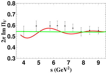
Therefore, we decided to proceed as follows. Since the problem with tau data is that they do not extend above $s=m^{2}_{\tau}$, we have supplemented these data with the spectral function from $e^{+}e^{-}$ in the range 4 GeV${}^{2}\lesssim s_{\min}\lesssim 9$ GeV² as provided by BES [20], at present the most precise (inclusive) measurement in this energy range. Inconsistencies between exclusive and inclusive determinations of the $e^{+}e^{-}$ cross section in the region 3 GeV${}^{2}\leq s\leq 4$ GeV² have prevented us from using these data as well. This is a longstanding issue (see, for instance, Ref. [21]) which, to the best of our knowledge, has not yet been fully resolved. Because of this, and because of all the extra assumptions we had to make to arrive at Eq. (6.1), we emphasize that the present exercise should be seen only as a very preliminary estimate of constraints from $e^{+}e^{-}$ data, rather than as a full-fledged analysis. For a more reliable analysis a better understanding of the theoretical aspects and better data in the $2-4$ GeV² window would be needed. The latter may soon be provided by BaBar [22].

With all these caveats in mind, we are now ready to address the question as to whether the values of the DV parameters in Eq. (4) are consistent with $e^{+}e^{-}$ data above $s=m^{2}_{\tau}$. To try answer this question, we have performed a combined fit in which we have taken the ansatz (4.1) to fit the tau data in the region $1.1$ GeV${}^{2}\lesssim s_{\min}\lesssim m^{2}_{\tau}$ and, simultaneously, the ansatz (6.1) to fit the $e^{+}e^{-}$ data in the region $4$ GeV${}^{2}\lesssim s_{\min}\lesssim 9$ GeV². The result of this combined fit yields the following values:

$$\kappa_{V} = 0.024\pm 0.004$$

$$\gamma_{V} = 0.40\pm 0.12$$

$$\alpha_{V} = 1.82\pm 0.19$$

$$\beta_{V} = 2.14\pm 0.11$$

$$\alpha^{\prime}_{V} = 5.2\pm 1.4$$

$$\frac{\chi^{2}}{dof} = \frac{22}{87}\simeq 0.25\ .$$ (6.2)

As one can see, our ansatz produces a reasonable fit to the data with values for the parameters which are compatible, within errors, with the results in Eq. (4). There is a certain trend towards smaller DVs, in comparison with our results from tau data alone. We note that if we compute the $\chi^{2}$ with the parameter values given in Eq. (6) using only the (nine) BES data points, we find a value $\chi^{2}/dof=10/9$. The comparison of the fits with the data, and with perturbation theory, can be seen in Fig. 4.

Using the values (6), we can estimate the DVs by substitution into Eq. (5.2), which yields

$$\delta R_{\tau}^{V}=-(0.0065\pm 0.0042)\ S_{EW}|V_{ud}|^{2}\ .$$ (6.3)

Following the same steps leading to Eq. (5.9), the corresponding shift in $\alpha_{s}$, as determined from the tau decay width, is given by

$$\delta\alpha_{s}(m_{\tau})\sim 0.001-0.003\ .$$ (6.4)

This value is roughly a factor three smaller than that previously found in the fit to tau data alone, Eq. (5.9), but it is not negligibly small in comparison with the theoretical errors quoted in Eq. (1).

7 Conclusions and outlook

In this work we have considered the problem of evaluating the possible size of DVs in tau decay. Even though there are good reasons to believe that DVs are present in QCD, our lack of understanding of these effects makes it very difficult to incorporate them in a systematic analysis of the data. However, ignoring the issue altogether may lead to a underestimation of systematic effects in the extraction of $\alpha_{s}$, quark masses and condensates. Some estimate of the effect of DVs is needed, given the high level of accuracy presently sought.

A general framework for the contribution of DVs is provided by Eqs. (2.8,2.9). In order to get to a quantitative estimate of DVs, however, more detailed information about the functions $\mathrm{Im}\Delta_{V,A}(s)$ is needed. In order to do this, we proposed an ansatz (3.1) which is based on the models of Refs. [14, 15, 16, 17], but which we expect to be of more general validity. Although this validity is speculative, at least it has the virtue of being falsifiable with future improvements in experimental data.

At present, the ansatz is perfectly compatible with the tau data, producing good fits for both the vector and the axial-vector spectral functions, and allowing us to determine the parameters of the ansatz, cf. Eqs. (4,4). These parameter values lead to the estimate (5.4) for the contribution from DVs to $R_{\tau}$, and, from that, to a possible theoretical error in $\alpha_{s}(m_{\tau})$ of order 0.003–0.010. Since we find good fits for both vector and axial-vector channels, our fits also give a good description of the $V+A$ spectral function. However, we find contributions to $R_{\tau}$ which are much larger than those based on a similar model in Ref. [5], which were obtained from an estimate based on the $V+A$ spectral function only.

Inclusion of $e^{+}e^{-}$ data, plus some assumptions, modifies the values of the parameters in the ansatz to those given in (6). These modified values lead to a reduction of the effect of DVs on $R_{\tau}$. This is just a consequence of the flatness of the inclusive $e^{+}e^{-}$ data above 4 GeV² [20], to which we have limited ourselves here, as they appear to be more reliable than the exclusive data at lower energies. However, given that exclusive data below 4 GeV² are not consistent with this behavior, it will be important to clarify this issue, once more and better data become available. At any rate, even with the inclusion of the $e^{+}e^{-}$ data of Ref. [20], we find that DVs may lead to a systematic error which is as large as $\delta\alpha_{s}(m_{\tau})|_{th}\simeq 0.003$, i.e., of the order of half the systematic errors from all other sources taken together in [5, 8], cf. Eq. (1). In a conservative approach, systematic errors with different origin ought to be added linearly. In light of these results, we conclude that future QCD analyses based on tau data should no longer neglect the possible contributions from DVs.

Acknowledgements

We thank Matthias Jamin for his collaboration at different stages of the present work, as well as for discussions. We would also like to thank Michel Davier, Sebastien Descotes-Genon, Andreas Höcker, Louis Lyons, Bogdan Malaescu, Kim Maltman, Ramón Miquel, Lluisa Mir, Antonio Pich, Eduardo de Rafael and Graziano Venanzoni for useful discussions. MG would like to thank IFAE at the UAB for hospitality. This work was supported in part by CICYT-FEDER-FPA2005-02211, SGR2005-00916, the Spanish Consolider-Ingenio 2010 Program CPAN (CSD2007-00042), by the EU Contract No. MRTN-CT-2006-035482, “FLAVIAnet,” and by the US Department of Energy.

Appendix: Estimate of OPE contributions to ${\mathrm{Im}}\,\Pi_{V,A}$

In the analysis of Sec. 4, the analytic form of the ansatz used to fit the spectral function, Eq. (4.1), assumed that the contribution from the OPE to the imaginary part of the correlator is negligible. In this appendix we will estimate the imaginary contributions coming from ${\cal{O}}(\alpha_{s})$ corrections from dimension four and six operators.

We start by splitting the vector and axial correlators as

$$\Pi_{V,A}=\Pi_{V,A}^{(0)}+\Pi_{V,A}^{(2)}+\Pi_{V,A}^{(4)}+\Pi_{V,A}^{(6)}\ ,$$ (A.1)

where the superscripts refer to the dimension of the OPE terms. The perturbative contributions are given by [1]

$$\Pi_{V}^{(0)}=\Pi_{A}^{(0)}=-\frac{1}{4\pi^{2}}\log{\frac{Q^{2}}{\mu^{2}}}\left[1+\frac{\alpha_{s}(Q)}{\pi}+\cdots\right]\ .$$ (A.2)

Contributions from $\Pi_{V,A}^{(2)}$ are proportional to the $u,d$ quark masses and can be safely neglected. The contribution from dimension four operators is, from Ref. [1]

$$Q^{4}\,\Pi_{V}^{(4)} = \frac{1}{12}\left[1-\frac{11}{18}\frac{\alpha_{s}(Q)}{\pi}+\cdots\right]\langle\frac{\alpha_{s}}{\pi}G_{\mu\nu}G^{\mu\nu}\rangle$$

$$+\left[1+\frac{13}{27}\frac{\alpha_{s}(Q)}{\pi}+\cdots\right](m_{u}+m_{d})\langle{\bar{\psi}}\psi\rangle+\frac{4}{27}\frac{\alpha_{s}(Q)}{\pi}\ m_{s}\langle{\bar{\psi}}\psi\rangle\;,$$

$$Q^{4}\,\Pi_{A}^{(4)} = \frac{1}{12}\left[1-\frac{11}{18}\frac{\alpha_{s}(Q)}{\pi}+\cdots\right]\langle\frac{\alpha_{s}}{\pi}G_{\mu\nu}G^{\mu\nu}\rangle$$

$$+\left[1-\frac{59}{27}\frac{\alpha_{s}(Q)}{\pi}+\cdots\right](m_{u}+m_{d})\langle{\bar{\psi}}\psi\rangle+\frac{4}{27}\frac{\alpha_{s}(Q)}{\pi}\ m_{s}\langle{\bar{\psi}}\psi\rangle\ ,$$

whereas for dimension six operators one finds [1]

$$Q^{6}\,\Pi_{V}^{(6)} = -8\pi^{2}\left[1-\frac{91}{72}\log{\frac{Q^{2}}{\mu^{2}}}\left(\frac{\alpha_{s}(\mu)}{\pi}\right)+\cdots\right]\left(\frac{\alpha_{s}(\mu)}{\pi}\right)\langle A_{\mu}^{a}A^{\mu\,a}\rangle$$

$$-\frac{32\pi^{2}}{9}\left[1-\frac{643}{288}\log{\frac{Q^{2}}{\mu^{2}}}\left(\frac{\alpha_{s}(\mu)}{\pi}\right)+\cdots\right]\left(\frac{\alpha_{s}(\mu)}{\pi}\right)\langle V_{\mu}^{a}V^{\mu\,a}\rangle$$

$$+\frac{16\pi^{2}}{27}\left[\log{\frac{Q^{2}}{\mu^{2}}}\left(\frac{\alpha_{s}(\mu)}{\pi}\right)^{2}+\cdots\right]\langle A_{\mu}A^{\mu}\rangle$$

$$+\frac{8\pi^{2}}{3}\left[\log{\frac{Q^{2}}{\mu^{2}}}\left(\frac{\alpha_{s}(\mu)}{\pi}\right)^{2}+\cdots\right]\langle V_{\mu}V^{\mu}\rangle\ ,$$

$$Q^{6}\,\Pi_{A}^{(6)} = \frac{55\pi^{2}}{9}\left[\log{\frac{Q^{2}}{\mu^{2}}}\left(\frac{\alpha_{s}(\mu)}{\pi}\right)^{2}+\cdots\right]\langle A_{\mu}^{a}A^{\mu\,a}\rangle$$ (A.4)

$$-\frac{88\pi^{2}}{9}\left[1-\frac{319}{792}\log{\frac{Q^{2}}{\mu^{2}}}\left(\frac{\alpha_{s}(\mu)}{\pi}\right)+\cdots\right]\left(\frac{\alpha_{s}(\mu)}{\pi}\right)\langle V_{\mu}^{a}V^{\mu\,a}\rangle$$

$$+\frac{88\pi^{2}}{27}\left[\log{\frac{Q^{2}}{\mu^{2}}}\left(\frac{\alpha_{s}(\mu)}{\pi}\right)^{2}+\cdots\right]\langle A_{\mu}A^{\mu}\rangle\ ,$$

where in all the equations above $(\cdots)$ stands for higher order contributions in the strong coupling constant. In the dimension six contribution we have kept only the leading log contribution (finite pieces will not contribute to the imaginary part), and we used the following short-hand notation for the four-quark condensates:

$$\langle A_{\mu}^{a}A^{\mu\,a}\rangle = \langle{\bar{\psi}}\gamma_{\mu}\gamma_{5}T^{a}\psi{\bar{\psi}}\gamma^{\mu}\gamma_{5}T^{a}\psi\rangle\ ,$$

$$\langle V_{\mu}^{a}V^{\mu\,a}\rangle = \langle{\bar{\psi}}\gamma_{\mu}T^{a}\psi{\bar{\psi}}\gamma^{\mu}T^{a}\psi\rangle\ ,$$

$$\langle A_{\mu}A^{\mu}\rangle = \langle{\bar{\psi}}\gamma_{\mu}\gamma_{5}\psi{\bar{\psi}}\gamma^{\mu}\gamma_{5}\psi\rangle\ ,$$

$$\langle V_{\mu}V^{\mu}\rangle = \langle{\bar{\psi}}\gamma_{\mu}\psi{\bar{\psi}}\gamma^{\mu}\psi\rangle\ .$$ (A.5)

Assuming vacuum factorization [2], the four-quark condensates simplify to

$$\langle A_{\mu}^{a}A^{\mu\,a}\rangle=-\langle V_{\mu}^{a}V^{\mu\,a}\rangle=\frac{4}{9}\langle{\bar{\psi}}\psi\rangle^{2}\ ,$$

$$\langle A_{\mu}A^{\mu}\rangle=-\langle V_{\mu}V^{\mu}\rangle=\frac{2}{9}\langle{\bar{\psi}}\psi\rangle^{2}\ .$$ (A.6)

In order to calculate ${\mathrm{Im}}\,\Pi_{V,A}(t)$, one uses that

$$\alpha_{s}(Q)=\alpha_{s}(\mu)\left\{1+\frac{\beta_{1}}{2}\frac{\alpha_{s}(\mu)}{\pi}\log{\frac{Q^{2}}{\mu^{2}}}\right\}\ ,$$ (A.7)

with

$$\beta_{1}=\frac{2n_{f}-11N_{c}}{6}\Bigg{|}_{n_{f}=3}=-\frac{9}{2}\ .$$ (A.8)

As a result,

$${\mathrm{Im}}\,[\alpha_{s}(Q)]=\frac{9}{4}[\alpha_{s}(Q)]^{2}\ .$$ (A.9)

It is now straightforward to calculate the different OPE contributions to the spectral functions. For normalization purposes it is convenient to work with $v_{1}\equiv 2\pi{\mathrm{Im}}\,\Pi_{V}$, $a_{1}\equiv 2\pi{\mathrm{Im}}\,\Pi_{A}$ . Taking $\alpha_{s}(1.1\,{\mathrm{GeV^{2}}})/\pi\simeq 0.15$, one finds for the perturbative contribution:

$$\delta v_{1}^{(0)}=\delta a_{1}^{(0)}=\frac{1}{2}\left[1+\frac{\alpha_{s}(Q)}{\pi}\right]\simeq 0.58\ .$$ (A.10)

Taking $\langle\alpha_{s}G^{2}\rangle\simeq 0.01\pi\,\,{\mathrm{GeV}}^{4}$, the gluon condensate contribution amounts to

$$\delta v_{1}^{(G^{2})}=\delta a_{1}^{(G^{2})}\simeq-4\cdot 10^{-4}\,\,\frac{{\mathrm{GeV}}^{4}}{Q^{4}}\ .$$ (A.11)

For the quark condensate contribution, we will assume SU(3) symmetry in the condensates, the PCAC relation $(m_{u}+m_{d})\langle{\bar{\psi}}\psi\rangle=-m_{\pi}^{2}f_{\pi}^{2}$, and estimate $m_{s}/(m_{u}+m_{d})\sim 10$. This yields

$$\delta v_{1}^{(\langle{\bar{\psi}}\psi\rangle)}\simeq-3\cdot 10^{-4}\,\,\frac{{\mathrm{GeV}}^{4}}{Q^{4}}\ ,\ \ \ \ \ \delta a_{1}^{(\langle{\bar{\psi}}\psi\rangle)}\simeq 1\cdot 10^{-4}\,\,\frac{{\mathrm{GeV}}^{4}}{Q^{4}}\ .$$ (A.12)

In Ref. [1] it was argued that the biggest non-perturbative contributions to $R_{\tau}$ come from the dimension six operators. There is some evidence that naive factorization does not work for these condensates. Based on a phenomenological fit, Ref. [1] concluded that there might be an enhancement over the result from factorization that can be represented by rescaling the condensate

$$\langle{\bar{\psi}}\psi\rangle^{2}\longrightarrow\lambda\langle{\bar{\psi}}\psi\rangle^{2}\ ,$$ (A.13)

where $\lambda$ is a fudge factor which, for typical values of $\alpha_{s}$ and the quark condensate, can be estimated to be $\lambda\simeq 3-9$. We take the quark condensate $\langle{\bar{\psi}}\psi\rangle=(-240\,{\mathrm{MeV}})^{3}$ and, to be conservative, we take $\lambda=10$. Accordingly,

$$\delta v_{1}^{(6,\lambda)}\lesssim 4\cdot 10^{-3}\,\,\frac{{\mathrm{GeV}}^{6}}{Q^{6}}\ ,\ \ \ \ \ \delta a_{1}^{(6,\lambda)}\lesssim-10^{-2}\,\,\frac{{\mathrm{GeV}}^{6}}{Q^{6}}\ .$$ (A.14)

Despite the enhancement by one order of magnitude, the contribution of dimension-six operators (as well as the dimension-four operators) is negligible compared to the perturbative contribution, Eq. (A.10). We conclude that we can safely neglect the contribution of the OPE to the spectral functions, in comparison to perturbation theory.

References

- [1] E. Braaten, S. Narison and A. Pich, Nucl. Phys. B 373, 581 (1992).
- [2] M. A. Shifman, A. I. Vainshtein and V. I. Zakharov, Nucl. Phys. B 147, 385 (1979).
- [3] S. Schael et al. [ALEPH Collaboration], Phys. Rept. 421, 191 (2005) [arXiv:hep-ex/0506072]; M. Davier, A. Höcker and Z. Zhang, Nucl. Phys. Proc. Suppl. 169, 22 (2007) [arXiv:hep-ph/0701170]; M. Davier, A. Höcker and Z. Zhang, Rev. Mod. Phys. 78, 1043 (2006) [arXiv:hep-ph/0507078].
- [4] S. Schael et al. [ALEPH Collaboration], Phys. Rept. 421, 191 (2005) [arXiv:hep-ex/0506072]. These data are available from http://aleph.web.lal.in2p3.fr/tau/specfun.html
- [5] M. Davier, S. Descotes-Genon, A. Höcker, B. Malaescu and Z. Zhang, Eur. Phys. J. C 56, 305 (2008) [arXiv:0803.0979 [hep-ph]].
- [6] P. A. Baikov, K. G. Chetyrkin and J. H. Kuhn, Phys. Rev. Lett. 101, 012002 (2008) [arXiv:0801.1821 [hep-ph]].
- [7] K. Maltman and T. Yavin, arXiv:0807.0650 [hep-ph].
- [8] M. Beneke and M. Jamin, JHEP 0809, 044 (2008) [arXiv:0806.3156 [hep-ph]].
- [9] F. Le Diberder and A. Pich, Phys. Lett. B 286, 147 (1992).
- [10] J. Bijnens, E. Gamiz and J. Prades, JHEP 0110 (2001) 009 [arXiv:hep-ph/0108240]; V. Cirigliano, E. Golowich and K. Maltman, Phys. Rev. D 68 (2003) 054013 [arXiv:hep-ph/0305118]; J. Rojo and J. I. Latorre, JHEP 0401 (2004) 055 [arXiv:hep-ph/0401047]; S. Narison, Phys. Lett. B 624 (2005) 223 [arXiv:hep-ph/0412152]; S. Friot, D. Greynat and E. de Rafael, JHEP 0410 (2004) 043 [arXiv:hep-ph/0408281]; K. N. Zyablyuk, Eur. Phys. J. C 38 (2004) 215 [arXiv:hep-ph/0404230]; C. A. Dominguez and K. Schilcher, JHEP 0701 (2007) 093 [arXiv:hep-ph/0611347]; A. A. Almasy, K. Schilcher and H. Spiesberger, arXiv:0802.0980 [hep-ph].
- [11] W. J. Marciano and A. Sirlin, Phys. Rev. Lett. 61, 1815 (1988); E. Braaten and C. S. Li, Phys. Rev. D 42, 3888 (1990); J. Erler, Rev. Mex. Fis. 50, 200 (2004) [arXiv:hep-ph/0211345].
- [12] R. Shankar, Phys. Rev. D 15, 755 (1977).
- [13] E. G. Floratos, S. Narison and E. de Rafael, Nucl. Phys. B 155, 115 (1979).
- [14] M. A. Shifman, arXiv:hep-ph/0009131.
- [15] B. Blok, M. A. Shifman and D. X. Zhang, Phys. Rev. D 57, 2691 (1998) [Erratum-ibid. D 59, 019901 (1999)] [arXiv:hep-ph/9709333]; I. I. Y. Bigi, M. A. Shifman, N. Uraltsev and A. I. Vainshtein, Phys. Rev. D 59, 054011 (1999) [arXiv:hep-ph/9805241].
- [16] O. Catà, M. Golterman and S. Peris, Phys. Rev. D 77, 093006 (2008) [arXiv:0803.0246 [hep-ph]].
- [17] O. Catà, M. Golterman and S. Peris, JHEP 0508, 076 (2005) [arXiv:hep-ph/0506004]. See also, M. Golterman, S. Peris, B. Phily and E. De Rafael, JHEP 0201, 024 (2002) [arXiv:hep-ph/0112042]; S. Peris, B. Phily and E. de Rafael, Phys. Rev. Lett. 86, 14 (2001) [arXiv:hep-ph/0007338].
- [18] C.M. Bender and S.A. Orszag, Advanced Mathematical Methods for Scientists and Engineers, Springer, 1999, Secs. 3.7 and 3.8.
- [19] Discussion session led by J. Donoghue at the workshop Matching light quarks to hadrons, Benasque Center for Science, Benasque, Spain, July-August 2004, http://benasque.ecm.ub.es/2004quarks/2004quarks.htm .
- [20] J. Z. Bai et al. [BES Collaboration], Phys. Rev. Lett. 88, 101802 (2002) [arXiv:hep-ex/0102003].
- [21] S. Eidelman and F. Jegerlehner, Z. Phys. C 67, 585 (1995) [arXiv:hep-ph/9502298].
- [22] Contribution by A. Denig at PHIPSI08, International Workshop on e+e- collisions from Phi to Psi, Laboratori Nazionali di Frascati, Italy, 7 - 10 April 2008, http://www.lnf.infn.it/conference/phipsi08/program/tuesday/lukin-denig.pdf .