The Isospectral Fruits of Representation Theory: Quantum Graphs and Drums

Abstract

We present a method which enables one to construct isospectral objects, such as quantum graphs and drums. One aspect of the method is based on representation theory arguments which are shown and proved. The complementary part concerns techniques of assembly which are both stated generally and demonstrated. For that purpose, quantum graphs are grist to the mill. We develop the intuition that stands behind the construction as well as the practical skills of producing isospectral objects. We discuss the theoretical implications which include Sunada’s theorem of isospectrality [2] arising as a particular case of this method. A gallery of new isospectral examples is presented and some known examples are shown to result from our theory.

1 Introduction

In 1966, Marc Kac asked his famous question, “Can one hear the shape of a drum?” [1]. This question can be rephrased as “does the Laplacian on every planar domain with Dirichlet boundary conditions have a unique spectrum?”. Ever since the time when Kac posed this fascinating question, physicists and mathematicians alike have attacked the problem from various angles. Attempts were made both to reconstruct the shape of an object from its spectrum, and to find different objects that are isospectral, i.e., have the same spectrum. The interested reader can find an elaborate summary of these efforts in [1]-[13]. In 1985, Sunada presented a theorem that describes a method to construct isospectral Riemannian manifolds [2]. Buser and later Berard expanded on this theorem, and offered a proof based on the concept of transplantation, as summarized by Brooks [3, 4, 5]. Over the years, several pairs of isospectral objects were found, but these were not planar domains, and therefore did not serve as an exact answer to Kac’s question. In 1992, by applying an extension of Sunada’s theorem, Gordon, Webb and Wolpert were able to finally answer Kac’s question as it related to drums, presenting the first pair of isospectral two-dimensional planar domains [6, 7]. Buser et al. later obtained a set of seventeen isospectral families of planar domains, both Neumann and Dirichlet isospectral [8]. Jakobson et al. and Levitin et al. extended the choice of boundary conditions by considering objects with alternating boundary conditions, and found sets of four planar domains that are mutually isospectral [9, 10]. In the late 1990’s, Gutkin and Smilansky reposed and answered Kac’s question as it applies to quantum graphs [24]. Recently, Band et al. presented a pair of isospectral quantum graphs [26], whose construction was generalized to the method described in this paper.

We begin by reviewing the terminology and the relevant definitions for quantum graphs. In section 3, we rederive the graphs constructed in [26], to help the reader gain an intuitive understanding of the method. Once the reader is familiar with the notions used, we formalize a theorem (section 4) along with a corollary, which together form the crux of the construction method. With the theorem in hand, we return to the basic example presented in section 3, and show that the isospectral pair can be expanded indefinitely $-$ section 5. After describing the assembly process rigorously in section 6, we devote section 7 to further investigating the theoretical implications of the theory. Finally, in sections 8, 9 we demonstrate how to apply the construction to other types of objects, and present a variety of examples of graphs, drums, and manifolds.

2 Quantum graphs

A graph $\Gamma$ consists of a finite set of vertices $V=\left\{v_{i}\right\}$ and a finite set $E=\left\{e_{j}\right\}$ of edges connecting the vertices. Each edge $e$ can be identified with a pair of vertices $\left\{v_{i},v_{k}\right\}$. We denote by $E_{v}$ the set of all edges incident to the vertex $v$. The degree (valency) of the vertex is $d_{v}=\left|E_{v}\right|$. This becomes a metric graph if each edge is assigned a finite length $l_{e}>0$. It is then possible to identify an edge $e$ with a finite segment $\left[0,l_{e}\right]$ of the real line having the natural coordinate $x_{e}$ along it. In this context, a function on the graph is a vector $f=\left(f\big{|}_{e_{1}},\ldots,f\big{|}_{e_{|E|}}\right)$ of functions $f\big{|}_{e_{j}}:\left[0,l_{e_{j}}\right]\rightarrow\mathbb{C}$ on the edges. Notice that in general it is not required that for $v\in V$ and $e,e^{\prime}\in E_{v}$ the functions $f\big{|}_{e}$ and $f\big{|}_{e^{\prime}}$ agree on $v$.

To obtain a quantum graph, we consider the following Hilbert space: $L^{2}\left(\Gamma\right)=\bigoplus_{j=1}^{\left|E\right|}L^{2}\left(\left[0,l_{e_{j}}\right]\right)$ with the inner product: $\left\langle f,g\right\rangle=\sum_{j=1}^{\left|E\right|}\int_{0}^{l_{e_{j}}}\overline{f\big{|}_{e_{j}}}\cdot g\big{|}_{e_{j}}\,dx_{e_{j}}$. The operator which draws our interest is the negative Laplacian: $-\bigtriangleup f=\left(-f^{\prime\prime}\Big{|}_{e_{1}},\ldots,-f^{\prime\prime}\Big{|}_{e_{\left|E\right|}}\right)$. The domain of definition for this operator is the Sobolev space, $W^{2,2}\left(\Gamma\right)$, the space of all functions $f$ such that $f\big{|}_{e_{j}}\in W^{2,2}\left(\left[0,l_{e_{j}}\right]\right)$ for all $1\leq j\leq\left|E\right|$. In addition we require the functions to obey certain boundary conditions stated a priori: for a vertex $v\in V$, we consider homogeneous boundary conditions which involve the function’s values and derivatives at the vertex, of the form $A_{v}\cdot f\Big{|}_{v}+B_{v}\cdot f^{\prime}\Big{|}_{v}=0$. Here $A_{v}$ and $B_{v}$ are $d_{v}\times d_{v}$ complex matrices, $f\Big{|}_{v}$ is the vector $\left(f\Big{|}_{e_{1}}(v),\ldots,f\Big{|}_{e_{d_{v}}}(v)\right)^{T}$ of the vertex values of the function along each edge incident to $v$, and $f^{\prime}\Big{|}_{v}=\left(f^{\prime}\Big{|}_{e_{1}}(v),\ldots,f^{\prime}\Big{|}_{e_{d_{v}}}(v)\right)^{T}$ is the vector of outgoing derivatives of $f$ taken at the vertex. Before stating the boundary conditions, the graph is merely a collection of independent edges with functions defined separately on each edge. The connectivity of the graph is manifested through the boundary conditions, which are local in nature: we relate the values of the function and its derivatives on each vertex, but no relation is assumed between those values on different vertices, or along the edges. In summary, a quantum graph is a metric graph equipped with a differential operator and with homogeneous differential boundary conditions at the vertices. One can generalize the metric Laplacian by including a potential or a magnetic flux defined on the edges. However, these generalizations will not be addressed here, and the interested reader is referred to the reviews [14, 15].

A standard choice of boundary condition which we adopt is the so called Neumann boundary condition:
$\bullet\quad$ $f$ agrees on the vertices: $\forall v\in V\quad\forall e,e^{\prime}\in E_{v}\,\,:\quad f\Big{|}_{e}\left(v\right)=f\Big{|}_{e^{\prime}}\left(v\right)$.
$\bullet\quad$ The sum of outgoing derivatives at each vertex is zero: $\forall v\in V$ :$\sum\limits_{e\in E_{v}}f^{\prime}\Big{|}_{e}\left(v\right)=0$.

It is worth noting that a Neumann vertex of valency two can be added at (or removed from) any point along an edge without changing the eigenspaces of the Laplacian, and thus, from a spectral point of view, without really changing the graph. Thus, loops (edges connecting a vertex to itself) and parallel edges (edges with the same endpoints) can be eliminated by the introduction of such “dummy” vertices $-$ we shall occasionally exploit this to simplify notation by assuming, without loss of generality, that we are dealing with graphs with no loops or parallel edges. A possible choice for matrices that correspond to the Neumann boundary conditions is:

$$A_{v}=\left(\begin{array}[]{cccc}1&-1\\ &\ddots&\ddots\\ &&1&-1\\ 0&\cdots&0&0\end{array}\right)\qquad B_{v}=\left(\begin{array}[]{cccc}0&0&\cdots&0\\ \vdots&\vdots&\ddots&\vdots\\ 0&0&\cdots&0\\ 1&1&\cdots&1\end{array}\right)\,.$$

For a vertex of degree one, the Neumann boundary condition is expressed by the matrices $A_{v}=\left(0\right),\,\,B_{v}=\left(1\right)$ and means that the derivative of the function equals zero at that vertex. Another useful boundary condition for a degree one vertex is the Dirichlet boundary condition, which means that the function vanishes at that vertex: $A_{v}=\left(1\right),\,\,B_{v}=\left(0\right)$. It can be seen that the Neumann condition renders the Laplacian self-adjoint, which guarantees that its spectrum is real. In general, Kostrykin and Schrader provide necessary and sufficient conditions that ensure the self-adjointness of the Laplacian: for every $v\in V$ the $d_{v}\times 2d_{v}$ matrix $\left(A_{v}\,B_{v}\right)$ must be of maximal rank $d_{v}$, and the matrix $A_{v}\cdot B_{v}^{\dagger}$ must be self-adjoint [16]. For a quantum graph $\Gamma$ we shall denote by $\Phi_{\Gamma}\left(\lambda\right)$ the space of complex functions on $\Gamma$ (i.e., satisfying the boundary conditions at the vertices) which are eigenfunctions of $\Gamma$’s (negative) Laplacian with eigenvalue $\lambda$:

$$\Phi_{\Gamma}\left(\lambda\right)=\left\{f\in W^{2,2}\left(\Gamma\right)\,|\,-\bigtriangleup f=\lambda f\right\}\,.$$ (2.1)

We define the spectrum of $\Gamma$ to be the function

$$\sigma_{\Gamma}:\lambda\mapsto\dim_{\mathbb{C}}\Phi_{\Gamma}\left(\lambda\right)\,,$$ (2.2)

which assigns to each eigenvalue its multiplicity. Two quantum graphs $\Gamma$ and $\Gamma^{\prime}$ are said to be isospectral if their spectra coincide, that is $\sigma_{\Gamma}\equiv\sigma_{\Gamma^{\prime}}$.

Quantum graphs play an important role in the study of quantum chaos. This connection was first revealed by the work of Kottos and Smilansky [17, 18]. They show that the spectral statistics of quantum graphs follow the predictions of random-matrix theory very closely. They propose a derivation of a trace formula for quantum graphs and point out its similarity to the famous Gutzwiller trace formula [19, 20] for chaotic Hamiltonian systems. The trace formula for a quantum graph connects the spectrum of the graph’s Laplacian to the total length of the graph and the lengths of its periodic orbits. The main result in the field of isospectrality of quantum graphs is that of Gutkin and Smilansky, [24], where they use the trace formula to show that under certain conditions a quantum graph can be heard, meaning that it can be recovered from the spectrum of its Laplacian. The necessary conditions include the graph being simple and its edges having rationally independent lengths. When these conditions are not satisfied, isospectral quantum graphs indeed arise. An early example appears in [21], in which Roth obtains isospectrality exploiting a spectral trace formula. vonBelow [22] uses the connection between spectra of discrete graphs and spectra of equilateral quantum graphs to turn isospectral discrete graphs into isospectral quantum graphs. In [23] isospectrality of weighted discrete graphs provides isospectral quantum graphs whose edges vary in length. A wealth of examples is constructed in [24, 25], using an analogy of the isospectral drums obtained by Buser et al. [8]. A recent example is the pair of isospectral dihedral graphs presented in [26]. Their construction was generalized to obtain the more complete theory which is presented in this paper.

3 A basic example

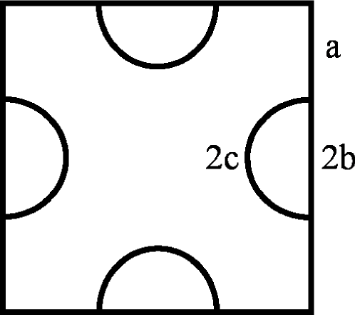
(a)

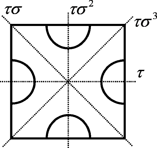
(b)

Figure 1: (a) A graph that obeys the dihedral symmetry of the square. The lengths of some edges are marked. (b) The same graph, showing the axes of the reflection elements in $D_{4}$.

Let $\Gamma$ be the graph given in figure 1(a). The lengths of the edges are determined by the parameters $a,b,c$ and we impose Neumann boundary conditions at all vertices. $G=D_{4}$, the dihedral group of the square, is the symmetry group of $\Gamma$. $G$ consists of the identity, three rotations and four reflections. Let $\tau$ denote the reflection of $\Gamma$ along the horizontal axis and $\sigma$ the rotation of $\Gamma$ counterclockwise by $\nicefrac{{\pi}}{{2}}$. The axes of the reflection elements in $G$ are shown in figure 1(b). We can describe $G$ and two of its subgroups $H_{1},H_{2}\leq G$ by:

$$G = \left<\sigma,\tau\right>=\{e,\,\sigma,\,\sigma^{2},\,\sigma^{3},\,\tau,\,\tau\sigma,\,\tau\sigma^{2},\,\tau\sigma^{3}\}$$

$$H_{1} = \left<\tau,\tau\sigma^{2}\right>=\{e,\,\tau,\,\tau\sigma^{2},\,\sigma^{2}\}$$

$$H_{2} = \left<\tau\sigma,\tau\sigma^{3}\right>=\{e,\,\tau\sigma,\,\tau\sigma^{3},\,\sigma^{2}\}$$

Consider the following one dimensional representations of $H_{1},H_{2}$, respectively:

$$R_{1} : \left\{\begin{array}[]{llll}e\mapsto\left(1\right),&\tau\mapsto\left(-1\right),&\tau\sigma^{2}\mapsto\left(1\right),&\sigma^{2}\mapsto\left(-1\right)\end{array}\right\}$$ (3.2)

$$R_{2} : \left\{\begin{array}[]{llll}e\mapsto\left(1\right),&\tau\sigma\mapsto\left(1\right),&\tau\sigma^{3}\mapsto\left(-1\right),&\sigma^{2}\mapsto\left(-1\right)\end{array}\right\}$$ (3.4)

We will use these representations to construct two graphs denoted by $\nicefrac{{\Gamma}}{{R_{1}}},\,\nicefrac{{\Gamma}}{{R_{2}}}$ (figure 2) which will be found to be isospectral.

(a)

(b)

Figure 2: The isospectral graphs (a) $\nicefrac{{\Gamma}}{{R_{1}}},\,$ (b) $\nicefrac{{\Gamma}}{{R_{2}}}$. Neumann boundary conditions are assumed if nothing else is specified. $D$ stands for Dirichlet boundary conditions and $N$ for Neumann.

We now explain the process of building the quotient graph $\nicefrac{{\Gamma}}{{R_{1}}}$. Let $\lambda\in\mathbb{C}$ and $\tilde{f}\in\Phi_{\Gamma}(\lambda)$ be a function which transforms according to the representation $R_{1}$, i.e.:

$$\forall g\in H_{1},\quad g\tilde{f}=\rho_{R_{1}}(g)\tilde{f}.$$ (3.5)

In the l.h.s., the action of the group $H_{1}$ on $\tilde{f}$ is by $\forall x\in\Gamma,\,\,(g\tilde{f})(x)=\tilde{f}(g^{-1}x)$. We use the transformation law of $\tilde{f}$ in order to deduce its properties: we know that $\tau\tilde{f}=-\tilde{f}$, which means that $\tilde{f}$ is an anti-symmetric function with respect to the horizontal reflection. We deduce that $\tilde{f}$ vanishes on the fixed points of $\tau$ (marked with diamonds in figure 3(a)). In a similar manner, we see that $\tilde{f}$ is symmetric with respect to the vertical reflection, since $\tau\sigma^{2}\tilde{f}=\tilde{f}$, and therefore the derivative of $\tilde{f}$ vanishes at the corresponding fixed points (the squares in figure 3(a)). Furthermore, it is enough to know the restriction of $\tilde{f}$ to the first quadrant (the bold subgraph in figure 3(a)) in order to deduce $\tilde{f}$ on the whole graph, using the known action of the reflections:

$$\tau\tilde{f}=-\tilde{f}\,,\quad\tau\sigma^{2}\tilde{f}=\tilde{f}\,.$$ (3.6)

Our construction process is now complete. The quotient graph $\nicefrac{{\Gamma}}{{R_{1}}}$ is the subgraph which lies in the first quadrant, with the boundary conditions of Dirichlet and Neumann in the appropriate locations, as was found for $\tilde{f}$ (figure 3(b)).

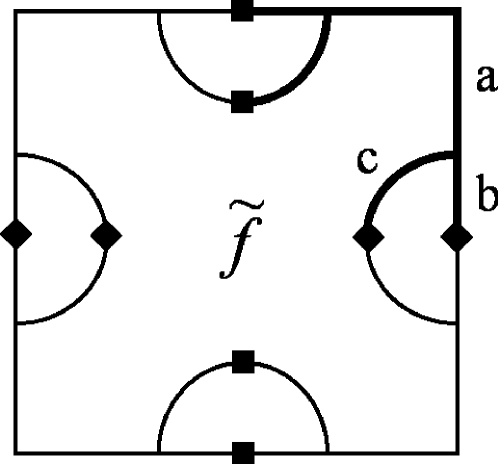
(a)

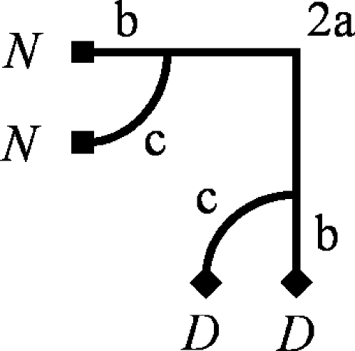
(b)

Figure 3: (a) The information we have on $\tilde{f}$ which transforms according to $R_{1}$. Diamonds mark the vertices at which the function vanishes and squares the vertices with zero derivative. (b) The quotient graph $\nicefrac{{\Gamma}}{{R_{1}}}$ which encodes this information. D stands for Dirichlet boundary conditions and N for Neumann.

From this example, we conclude that the construction of the quotient graph is motivated by an encoding scheme. We choose a fundamental domain for the action of $G$ on $\Gamma$, i.e., a minimal subgraph from which the entire graph can be reached by the action of the group. We take this domain to be the quotient graph $\nicefrac{{\Gamma}}{{R_{1}}}$. We encode a function $\tilde{f}\in\Phi_{\Gamma}(\lambda)$, which transforms according to the representation $R_{1}$, by a function $f\in\Phi_{\nicefrac{{\Gamma}}{{R_{1}}}}(\lambda)$. The encoding is described by the map $\Psi:\Phi_{\Gamma}^{R_{1}}(\lambda)\rightarrow\Phi_{\nicefrac{{\Gamma}}{{R_{1}}}}(\lambda)$, where $\Phi_{\Gamma}^{R_{1}}(\lambda)$ is the space of all functions $\tilde{f}\in\Phi_{\Gamma}(\lambda)$ that transform according to the representation $R_{1}$, and $\Psi$ is just the restriction map to the fundamental domain. An important observation is that given $f\in\Phi_{\nicefrac{{\Gamma}}{{R_{1}}}}(\lambda)$, it is possible to construct a unique function $\tilde{f}\in\Phi_{\Gamma}^{R_{1}}(\lambda)$ (using (3.6)), whose restriction to the fundamental domain is $f$ (this is the decoding process). It follows that $\Psi$ is invertible and thus is an isomorphism:

$$\Phi_{\Gamma}^{R_{1}}(\lambda)\cong\Phi_{\nicefrac{{\Gamma}}{{R_{1}}}}(\lambda)$$ (3.7)

The quotient $\nicefrac{{\Gamma}}{{R_{2}}}$ is constructed similarly. For any $\lambda\in\mathbb{C}$, we consider $\tilde{f}\in\Phi_{\Gamma}^{R_{2}}(\lambda)$, which means that $\tilde{f}$ transforms in the following way:

$$\tau\sigma\tilde{f}=\tilde{f}\,,\quad\tau\sigma^{3}\tilde{f}=-\tilde{f}$$ (3.8)

and carry on with the same arguments as above. We do not specify the details of this process but rather summarize it in figure 4.

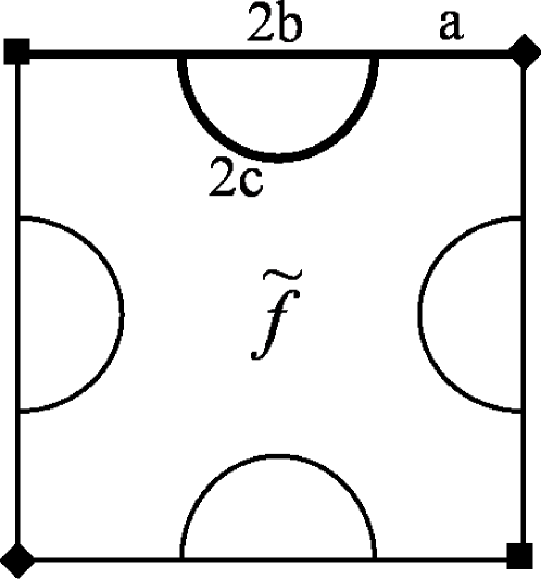
(a)

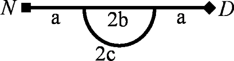
(b)

Figure 4: (a) The information we have on $\tilde{f}\in\Phi_{\Gamma}^{R_{2}}(\lambda)$. Diamonds mark the vertices at which the function vanishes and squares the vertices with zero derivative. (b) The quotient graph $\nicefrac{{\Gamma}}{{R_{2}}}$ which encodes this information. D stands for Dirichlet boundary conditions and N for Neumann.

The isospectrality of $\nicefrac{{\Gamma}}{{R_{1}}}$ and $\nicefrac{{\Gamma}}{{R_{2}}}$ is a direct consequence of corollary 4.4 which appears in the next section.

4 Representation theory and isospectrality

Having informally exposed some of the relations between representations and quantum graphs, we begin a more precise examination, culminating in a general theorem on isospectrality . Let $\Gamma$ be a graph that obeys a certain finite symmetry group $G$; this means that the action of $G$ preserves the lengths of the edges and the connectivity and boundary conditions at the vertices. We do not assume that $G$ is the maximal symmetry group of $\Gamma$. For every $\lambda\in\mathbb{C}$, $\Phi_{\Gamma}\left(\lambda\right)$, the vector space of all $\lambda$-eigenfunctions of the Laplacian on $\Gamma$, is a carrier space of some representation of $G$. This follows from the Laplacian commuting with the symmetry group: $\forall g\in G,\,\,-\bigtriangleup(gf)=g\left(-\bigtriangleup f\right)=\lambda(gf)$, which renders $\Phi_{\Gamma}\left(\lambda\right)$ closed under the action of $G$. Let $R$ denote the representation carried by $\Phi_{\Gamma}\left(\lambda\right)$, and decompose it into the irreducible representations of $G$. Such a decomposition allows us to present $\Phi_{\Gamma}\left(\lambda\right)$ as some direct sum of carrier spaces of the irreducible representations of $G$. Denote by $S_{1},\ldots,S_{r}$ the irreducible representations of $G$ and assume that $S_{i}$ appears $n_{i}$ times in $R$, i.e., $R\cong\bigoplus_{i=1}^{r}n_{i}\,S_{i}$. Then

$$\Phi_{\Gamma}\left(\lambda\right) = \left(V_{1}^{S_{1}}\oplus\ldots\oplus V_{n_{1}}^{S_{1}}\right)\oplus\ldots\oplus\left(V_{1}^{S_{r}}\oplus\ldots\oplus V_{n_{r}}^{S_{r}}\right)$$ (4.1)

$$= \bigoplus_{i=1}^{r}\>\Phi_{\Gamma}^{S_{i}}\left(\lambda\right)\,,$$

where, for each $i\in\left\{1..r\right\}$, $\left\{V_{j}^{S_{i}}\right\}_{j=1}^{n_{i}}$ are carrier spaces of the irreducible representation $S_{i}$ (one carrier space for each copy of $S_{i}$ in $R$), and their direct sum in $\Phi_{\Gamma}\left(\lambda\right)$ is denoted by $\Phi_{\Gamma}^{S_{i}}\left(\lambda\right)$. $\Phi_{\Gamma}^{S_{i}}\left(\lambda\right)$ is called the $S_{i}$-isotypic component of $\Phi_{\Gamma}\left(\lambda\right)$; it is the vector space consisting of all $\lambda$-eigenfunctions which transform under the action of $G$ according to the representation $S_{i}$. Denoting by $\mathbf{1}_{G}$ the trivial representation of $G$, $\Phi_{\Gamma}^{\mathbf{1}_{G}}\left(\lambda\right)$ is called the trivial component of $\Phi_{\Gamma}\left(\lambda\right)$, and is the space of all $\lambda$-eigenfunctions which are invariant under the action of $G$.

We pause the algebraic discussion for the purpose of reexamining the example from the previous section. Recall that $R_{1}$ is a representation of the group $H_{1}$, and that we have constructed a quotient graph $\nicefrac{{\Gamma}}{{R_{1}}}$, such that the following isomorphisms were established:

$$\forall\lambda\in\mathbb{C},\quad\Psi:\Phi_{\Gamma}^{R_{1}}\left(\lambda\right)\binrel@{\longrightarrow}\binrel@@{\mathop{\kern 0.0pt\longrightarrow}\limits^{\cong}}\Phi_{\nicefrac{{\Gamma}}{{R_{1}}}}\left(\lambda\right)$$ (4.2)

By definition, the dimension of $\Phi_{\nicefrac{{\Gamma}}{{R_{1}}}}\left(\lambda\right)$ is $\sigma_{\nicefrac{{\Gamma}}{{R_{1}}}}(\lambda)$, the multiplicity of $\lambda$ in the spectrum of $\nicefrac{{\Gamma}}{{R_{1}}}$. In analogy, we denote by $\sigma_{\Gamma}^{R_{1}}\left(\lambda\right)$ the dimension of $\Phi_{\Gamma}^{R_{1}}\left(\lambda\right)$. But what does this dimension tell us? It can be thought of as the spectrum that will be observed by someone who can only see functions which transform according to $R_{1}$. We call $\sigma_{\Gamma}^{R_{1}}$ the $R_{1}$-spectrum of $\Gamma$, and note in particular that it is a subspectrum of $\Gamma$: $\sigma_{\Gamma}^{R_{1}}\leq\sigma_{\Gamma}$. In terms of dimensions (4.2) gives

$$\sigma_{\Gamma}^{R_{1}}\equiv\sigma_{\nicefrac{{\Gamma}}{{R_{1}}}}\,.$$ (4.3)

We thus identify the role of the quotient graph $\nicefrac{{\Gamma}}{{R_{1}}}$ as having the same spectrum as the $R_{1}$-spectrum of the original graph. This will be the characterizing property of all our quotient graphs, and it is therefore time to generalize the discussion.

As we have defined the $R_{1}$-spectrum by $\sigma_{\Gamma}^{R_{1}}(\lambda)=\dim\Phi_{\Gamma}^{R_{1}}(\lambda)$, we now define the $S$-spectrum of $\Gamma$, for any irreducible representation $S$ (not necessarily one dimensional), as

$$\sigma_{\Gamma}^{S}(\lambda):=\frac{{\rm dim}\Phi_{\Gamma}^{S}(\lambda)}{{\rm dim}S}\,,$$ (4.4)

which can be interpreted as the number of copies of $S$ of which $\Phi_{\Gamma}^{S}\left(\lambda\right)$ consists. This is also equal to the number of copies of $S$ in $\Phi_{\Gamma}(\lambda)$ (the corresponding $n_{i}$ in (4.1)). Using the orthogonality relations of irreducible characters, we may rewrite (4.4) as $\sigma_{\Gamma}^{S}\left(\lambda\right)=\left\langle\chi_{S},\chi_{\Phi_{\Gamma}\left(\lambda\right)}\right\rangle_{G}$. We use this equality to generalize the definition:

Definition 4.1.

For any representation $R$, the $R$-spectrum of $\Gamma$ is

$$\sigma_{\Gamma}^{R}(\lambda):=\left\langle\chi_{R},\chi_{\Phi_{\Gamma}\left(\lambda\right)}\right\rangle_{G}\,.$$ (4.5)

Note that (4.4) holds for irreducible representations and is not true for all $R$ (in fact, $\Phi^{R}_{\Gamma}(\lambda)$ is not even defined when $R$ is reducible). Equipped with the notion of the $R$-spectrum of $\Gamma$, we can now define what is a $\nicefrac{{\Gamma}}{{R}}$ graph.

Definition 4.2.

A $\nicefrac{{\Gamma}}{{R}}$-graph is any quantum graph $\Gamma^{\prime}$ whose spectrum is equal to the $R$-spectrum of $\Gamma$:

$$\sigma_{\Gamma^{\prime}}\equiv\sigma_{\Gamma}^{R}\,.$$

Since all $\nicefrac{{\Gamma}}{{R}}$-graphs have the same spectrum by definition, we allow ourselves, by abuse of language, to refer to the spectrum of $\nicefrac{{\Gamma}}{{R}}$. The following isospectrality theorem then follows:

Theorem 4.3.

Let $\Gamma$ be a quantum graph equipped with an action of a group $G$, $H$ a subgroup of $G$, and $R$ a representation of $H$. Then $\nicefrac{{\Gamma}}{{R}}$ is isospectral to $\nicefrac{{\Gamma}}{{{\rm Ind}_{H}^{G}R}}$.

Proof.

$$\forall\lambda\in\mathbb{C}\qquad\sigma_{\Gamma/R}(\lambda)=\sigma_{\Gamma}^{R}(\lambda) = \langle\chi_{R}\,,\,\chi_{\Phi_{\Gamma}(\lambda)}\rangle_{H}$$

$$= \langle\chi_{{\rm Ind}_{H}^{G}R}\,,\,\chi_{\Phi_{\Gamma}(\lambda)}\rangle_{G}$$

$$= \sigma_{\Gamma}^{{\rm Ind}_{H}^{G}R}(\lambda)=\sigma_{\Gamma/{{\rm Ind}_{H}^{G}R}}(\lambda)$$

where moving to the second line we have used the Frobenius Reciprocity Theorem. ∎

Corollary 4.4.

If $G$ acts on $\Gamma$ and $H_{1},H_{2}$ are subgroups of $G$ with corresponding representations $R_{1},R_{2}$ such that ${\rm Ind}_{H_{1}}^{G}R_{1}\cong{\rm Ind}_{H_{2}}^{G}R_{2}$, then $\nicefrac{{\Gamma}}{{R_{1}}}$ and $\nicefrac{{\Gamma}}{{R_{2}}}$ are isospectral.

Remark.

This corollary is in fact equivalent to the theorem, as can be seen by taking $H_{2}=G$, $R_{2}={\rm Ind}_{H_{1}}^{G}R_{1}$.

The isospectrality of the pair of graphs constructed in section 3 (figure 2) is obtained from the above corollary. Returning to that example, one first notices that the two graphs presented there obey definition 4.2. This is true since we have shown that

$$\forall\lambda\in\mathbb{C}\quad\Phi_{\nicefrac{{\Gamma}}{{R_{1}}}}(\lambda)\cong\Phi_{\Gamma}^{R_{1}}(\lambda)$$

from which follows $\sigma_{\nicefrac{{\Gamma}}{{R_{1}}}}\equiv\sigma_{\Gamma}^{R_{1}}$ and therefore the first graph presented in section 3 can be honestly called a $\nicefrac{{\Gamma}}{{R_{1}}}$-graph. The same goes for the second graph, $\nicefrac{{\Gamma}}{{R_{2}}}$. The representations $R_{1},R_{2}$ used in the construction satisfy the condition ${\rm Ind}_{H_{1}}^{G}R_{1}\cong{\rm Ind}_{H_{2}}^{G}R_{2}$ and this enables us to apply corollary 4.4 and conclude that $\nicefrac{{\Gamma}}{{R_{1}}}$ and $\nicefrac{{\Gamma}}{{R_{2}}}$ are isospectral.

5 Extending the basic example

It is clear that theorem 4.3 and corollary 4.4 would yield isospectral examples only when the required quotient graphs indeed exist. We saw the existence of two such quotients in section 3. A proof of the existence of the quotient of any graph by any representation, along with a rigorous construction technique, are given in [27]. In this section, we present key examples which enable us to gain insight into this method, as well as to understand the procedure implemented in [27].

We return to the basic example brought forth in section 3, wishing to extend it by discovering more quantum graphs which are isospectral to the pair of graphs $\nicefrac{{\Gamma}}{{R_{1}}},\nicefrac{{\Gamma}}{{R_{2}}}$ in figure 2. Corollary 4.4 offers a method by which this can be achieved: find a subgroup $H_{3}\leq G$ and a representation $R_{3}$ of it such that ${\rm Ind}_{H_{1}}^{G}R_{1}\cong{\rm Ind}_{H_{2}}^{G}R_{2}\cong{\rm Ind}_{H_{3}}^{G}R_{3}$. Then, $\nicefrac{{\Gamma}}{{R_{3}}}$ is isospectral to $\nicefrac{{\Gamma}}{{R_{1}}}$ and $\nicefrac{{\Gamma}}{{R_{2}}}$. Such a subgroup and a representation indeed exist:

$$H_{3} = \{e,\,\sigma,\,\sigma^{2},\,\sigma^{3}\}$$

$$R_{3} : \left\{\begin{array}[]{llll}e\mapsto\left(1\right),&\sigma\mapsto\left(i\right),&\sigma^{2}\mapsto\left(-1\right),&\sigma^{3}\mapsto\left(-i\right)\end{array}\right\}$$ (5.2)

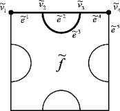
(a)

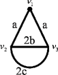
$A_{v_{1}}=\left(\begin{array}[]{cc}1&-i\\ 0&0\end{array}\right)$

$B_{v_{1}}=\left(\begin{array}[]{cc}0&0\\ 1&i\end{array}\right)$

(b)

Figure 5: (a) The information we have on $\tilde{f}\in\Phi_{\Gamma}^{R_{3}}\left(\lambda\right)$. There is a factor of $i$ between the values and the clockwise derivatives of $\tilde{f}$ at the marked vertices $\tilde{v}_{1},\tilde{v}_{4}$. (b) The quotient graph $\nicefrac{{\Gamma}}{{R_{3}}}$ which encodes this information. The only non-Neumann boundary condition is at $v_{1}$ and it is specified by the matrices $A_{v_{1}},\,B_{v_{1}}$.

We use the intuitive approach obtained from the basic example in order to construct the quotient $\nicefrac{{\Gamma}}{{R_{3}}}$. Let $\tilde{f}$ be a function that transforms according to the representation $R_{3}$. The action of the rotation element $\sigma$ on $\tilde{f}$ is given by

$$\sigma\,\tilde{f}=i\,\tilde{f}.$$ (5.3)

This means that knowing the values of $\tilde{f}$ on a quarter of the graph (for example, the quarter marked in bold in figure 5(a)) enables us to deduce the values of $\tilde{f}$ on the whole of $\Gamma$. We therefore take this subgraph to be our quotient graph and check what boundary conditions we should impose on it. From (5.3) we obtain

$$\tilde{f}\Big{|}_{\tilde{e}^{1}}(\tilde{v}_{1}) = i\,\tilde{f}\Big{|}_{\tilde{e}^{5}}(\tilde{v}_{4})$$ (5.4)

$$\tilde{f}^{\prime}\Big{|}_{\tilde{e}^{1}}(\tilde{v}_{1}) = i\,\tilde{f}^{\prime}\Big{|}_{\tilde{e}^{5}}(\tilde{v}_{4})\,.$$ (5.5)

These equations suggest that we should identify vertices $\tilde{v}_{1},\tilde{v}_{4}$. They merge to become a single vertex $v_{1}$ in the quotient (figure 5(b)). Equation (5.4) gives the boundary condition for the values at this new vertex. The boundary condition for the derivatives at $v_{1}$ is obtained from (5.5), by recalling that $\tilde{f}$ obeys Neumann boundary conditions at the vertex $\tilde{v}_{4}$ of $\Gamma$:

$$\tilde{f}^{\prime}\Big{|}_{\tilde{e}^{4}}(\tilde{v}_{4})+\tilde{f}^{\prime}\Big{|}_{\tilde{e}^{5}}(\tilde{v}_{4})=0\,.$$ (5.6)

Therefore, the boundary conditions at $v_{1}$ in $\nicefrac{{\Gamma}}{{R_{3}}}$ are described by the matrices given in figure 5(b), and this concludes the construction of $\nicefrac{{\Gamma}}{{R_{3}}}$. The isomorphisms

$$\forall\lambda\in\mathbb{C},\quad\Psi:\Phi_{\Gamma}^{R_{3}}\left(\lambda\right)\binrel@{\longrightarrow}\binrel@@{\mathop{\kern 0.0pt\longrightarrow}\limits^{\cong}}\Phi_{\nicefrac{{\Gamma}}{{R_{3}}}}\left(\lambda\right)$$ (5.7)

can be easily deduced from the construction process. Taking dimensions gives $\sigma_{\Gamma}^{R_{3}}~{}\equiv~{}\sigma_{\nicefrac{{\Gamma}}{{R_{3}}}}$, which proves the validity of this quotient.

We already obtained an isospectral triple, but this does not cause us to stagnate and we go further with our isospectral quest. By theorem 4.3, any $\nicefrac{{\Gamma}}{{R}}$-graph, where $R\cong{\rm Ind}_{H_{1}}^{G}R_{1}$, would be isospectral to our three graphs. A simple calculation (See A) shows that $R$ is the single two dimensional irreducible representation of $G=D_{4}$. By a choice of basis we can describe $R$ as a matrix representation. Such a representation is:

$$\left\{\begin{array}[]{cccc}e\mapsto{\scriptsize\left(\begin{array}[]{cc}1&0\\ 0&1\end{array}\right)},&\sigma\mapsto{\scriptsize\left(\begin{array}[]{cc}0&1\\ -1&0\end{array}\right)},&\sigma^{2}\mapsto{\scriptsize\left(\begin{array}[]{cc}-1&0\\ 0&-1\end{array}\right)},&\sigma^{3}\mapsto{\scriptsize\left(\begin{array}[]{cc}0&-1\\ 1&0\end{array}\right)},\\ \\ \tau\mapsto{\scriptsize\left(\begin{array}[]{cc}-1&0\\ 0&1\end{array}\right)},&\tau\sigma\mapsto{\scriptsize\left(\begin{array}[]{cc}0&-1\\ -1&0\end{array}\right)},&\tau\sigma^{2}\mapsto{\scriptsize\left(\begin{array}[]{cc}1&0\\ 0&-1\end{array}\right)},&\tau\sigma^{3}\mapsto{\scriptsize\left(\begin{array}[]{cc}0&1\\ 1&0\end{array}\right)}\end{array}\right\}$$ (5.8)

We now construct the quotient $\nicefrac{{\Gamma}}{{R}}$. The graph obtained, which is shown in figure 6(b) is the same as $\nicefrac{{\Gamma}}{{R_{1}}}$ (figure 2(a)) and we elaborate on this phenomenon later on. The construction process of this “new” graph is now presented for didactic reasons. The procedure is similar to those already described, although a slight complication arises from $R$ not being one dimensional.

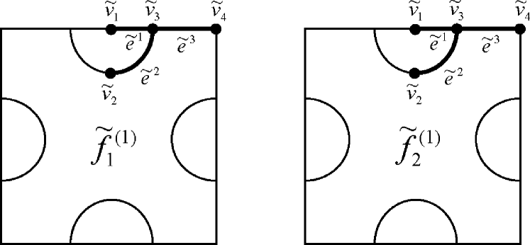
(a)

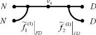
(b)

Figure 6: (a) Two copies of the graph $\Gamma$ which assist in the visualization of the functions $\tilde{f}_{1}^{(1)},\tilde{f}_{2}^{(1)}$ on $\Gamma$. The fundamental domain is marked in bold. (b) The quotient graph $\nicefrac{{\Gamma}}{{R}}$ formed as two copies of the fundamental domain.

We consider two functions $\tilde{f}_{1}^{(1)},\tilde{f}_{2}^{(1)}\in\Phi_{\Gamma}(\lambda)$ (for some $\lambda\in\mathbb{C}$) that transform according to the matrix representation (5.8). It follows that $\tilde{f}_{1}^{(1)},\tilde{f}_{2}^{(1)}\in\Phi_{\Gamma}^{R}(\lambda)$, and that $\tilde{f}_{1}^{(1)}$ and $\tilde{f}_{2}^{(1)}$ form a basis for a carrier space of the representation $R$, which we denote by $V_{1}^{R}$. We may proceed in this manner, choosing $\tilde{f}_{1}^{\left(2\right)},\tilde{f}_{2}^{\left(2\right)},\ldots$ such that each pair, $\left\{\tilde{f}_{1}^{\left(i\right)},\tilde{f}_{2}^{\left(i\right)}\right\}$, transforms according to (5.8), and is linearly independent of the previous ones. Therefore, each pair, $\left\{\tilde{f}_{1}^{\left(i\right)},\tilde{f}_{2}^{\left(i\right)}\right\}$, spans a different carrier space of $R$, which we denote by $V_{i}^{R}$ and we get that $\Phi_{\Gamma}^{R}\left(\lambda\right)=\bigoplus\limits_{i=1}^{n}V_{i}^{R}$. The number of carrier spaces is

$$n=\frac{\dim\Phi_{\Gamma}^{R}\left(\lambda\right)}{\dim R}=\left\langle\chi_{R},\chi_{\Phi_{\Gamma}^{R}\left(\lambda\right)}\right\rangle_{G}=\left\langle\chi_{R},\chi_{\Phi_{\Gamma}\left(\lambda\right)}\right\rangle_{G}=\sigma_{\Gamma}^{R}(\lambda)\,$$ (5.9)

(recall that $R$ is irreducible). We wish to construct a quotient $\nicefrac{{\Gamma}}{{R}}$ such that

$$\dim\Phi_{\nicefrac{{\Gamma}}{{R}}}(\lambda)=n\,,$$ (5.10)

which means that $\sigma_{\nicefrac{{\Gamma}}{{R}}}(\lambda)=\sigma_{\Gamma}^{R}(\lambda)$. If this holds for every $\lambda$, then $\nicefrac{{\Gamma}}{{R}}$ is indeed the desired quotient graph (definition 4.2). If we again relate the construction process to the encoding technique, we see that we can achieve (5.10) if each carrier space $V_{i}^{R}$ is encoded by a single function $f^{(i)}\in\Phi_{\nicefrac{{\Gamma}}{{R}}}(\lambda)$, in a manner that $\left\{f^{(i)}\right\}_{i=1}^{n}$ is a basis for $\Phi_{\nicefrac{{\Gamma}}{{R}}}\left(\lambda\right)$. We demonstrate this idea by encoding $V_{1}^{R}={\rm Span}\left\{\tilde{f}_{1}^{(1)},\tilde{f}_{2}^{(1)}\right\}$. This is done by thinking of the basis functions $\tilde{f}_{1}^{(1)},\tilde{f}_{2}^{(1)}$ as residing on two copies of the graph $\Gamma$ (figure 6(a)). Knowing the values of $\tilde{f}_{1}^{(1)}$ and $\tilde{f}_{2}^{(1)}$ on a fundamental domain for the action of $G$ on $\Gamma$ (e.g., the bold subgraphs in figure 6(a)) allows one to deduce the values of $\tilde{f}_{1}^{(1)}$ and $\tilde{f}_{2}^{(1)}$ on the whole graph, using the known action of the group (5.8). Therefore, the quotient graph is the union of these two copies of the fundamental domain. Its boundary conditions can be concluded from (5.8), which gives the relations between the values of $\tilde{f}_{1}^{(1)},\tilde{f}_{2}^{(1)}$ and between their derivatives:

$$\tau\sigma^{2}\,\tilde{f}_{1}^{(1)}=\tilde{f}_{1}^{(1)} \quad\Rightarrow\quad \left(\tilde{f}_{1}^{(1)}\right)^{\prime}\Big{|}_{\tilde{e}^{1}}(\tilde{v}_{1})=\left(\tilde{f}_{1}^{(1)}\right)^{\prime}\Big{|}_{\tilde{e}^{2}}(\tilde{v}_{2})=0$$ (5.11)

$$\tau\sigma^{2}\,\tilde{f}_{2}^{(1)}=-\tilde{f}_{2}^{(1)} \quad\Rightarrow\quad \tilde{f}_{2}^{(1)}\Big{|}_{\tilde{e}^{1}}(\tilde{v}_{1})=\tilde{f}_{2}^{(1)}\Big{|}_{\tilde{e}^{2}}(\tilde{v}_{2})=0$$ (5.12)

$$\tau\sigma^{3}\,\tilde{f}_{1}^{(1)}=\tilde{f}_{2}^{(1)}$$ . (5.13)

We recall that $\tilde{f}_{1}^{(1)}$ satisfies Neumann boundary conditions at $\tilde{v}_{4}$:

$$\left(\tau\sigma^{3}\tilde{f}_{1}^{(1)}\right)\Big{|}_{\tilde{e}^{3}}(\tilde{v}_{4})=\tilde{f}_{1}^{(1)}\Big{|}_{\tau\sigma^{3}\tilde{e}^{3}}(\tilde{v}_{4})=\tilde{f}_{1}^{(1)}\Big{|}_{\tilde{e}^{3}}(\tilde{v}_{4})$$ (5.14)

$$\left(\tau\sigma^{3}\tilde{f}_{1}^{(1)}\right)^{\prime}\Big{|}_{\tilde{e}^{3}}(\tilde{v}_{4})=\left(\tilde{f}_{1}^{(1)}\right)^{\prime}\Big{|}_{\tau\sigma^{3}\tilde{e}^{3}}(\tilde{v}_{4})=-\left(\tilde{f}_{1}^{(1)}\right)^{\prime}\Big{|}_{\tilde{e}^{3}}(\tilde{v}_{4})\quad.$$ (5.15)

Plugging (5.13) into (5.14), (5.15), gives the following relations:

$$\tilde{f}_{2}^{(1)}\Big{|}_{\tilde{e}^{3}}(\tilde{v}_{4})=\tilde{f}_{1}^{(1)}\Big{|}_{\tilde{e}^{3}}(\tilde{v}_{4})$$ (5.16)

$$\left(\tilde{f}_{2}^{(1)}\right)^{\prime}\Big{|}_{\tilde{e}^{3}}(\tilde{v}_{4})=-\left(\tilde{f}_{1}^{(1)}\right)^{\prime}\Big{|}_{\tilde{e}^{3}}(\tilde{v}_{4})\quad.$$ (5.17)

Equations (5.16) and (5.17) motivate us to glue the two sub-graphs at the vertex $\tilde{v}_{4}$ and supplement the new graph with Neumann boundary conditions at this vertex, which we denote by $v_{4}$. The relations (5.11), (5.12) give Neumann and Dirichlet boundary conditions, respectively, on the other vertices, and this fully describes the quotient graph $\nicefrac{{\Gamma}}{{R}}$ (figure 6(b)).

We now explain how this encoding enables us to prove that $\sigma_{\nicefrac{{\Gamma}}{{R}}}\equiv\sigma_{\Gamma}^{R}$, and ensure the validity of our $\nicefrac{{\Gamma}}{{R}}$. Given $\tilde{f}_{1}^{(1)},\tilde{f}_{2}^{(1)}$ as above, we form a function $f^{(1)}\in\Phi_{\nicefrac{{\Gamma}}{{R}}}(\lambda)$ whose left half is equal to the restriction of $\tilde{f}_{1}^{(1)}$ to the fundamental domain, and whose right half is the restriction of $\tilde{f}_{2}^{(1)}$ to the fundamental domain. The considerations above apply for every carrier space $V_{i}^{R}$, and we can encode its basis $\left\{\tilde{f}_{1}^{(i)},\tilde{f}_{2}^{(i)}\right\}$ by a function $f^{(i)}\in\Phi_{\nicefrac{{\Gamma}}{{R}}}(\lambda)$ in the same way as was done for $i=1$.

The set $\bigcup\limits_{i=1}^{n}\left\{\tilde{f}_{1}^{(i)},\tilde{f}_{2}^{(i)}\right\}$ forms a basis for $\Phi_{\Gamma}^{R}(\lambda)$, and is therefore linearly independent. We now show that $\left\{f^{(i)}\right\}_{i=1}^{n}$ are linearly independent as well, which gives $\frac{1}{2}\dim\Phi_{\Gamma}^{R}(\lambda)\leq\dim\Phi_{\nicefrac{{\Gamma}}{{R}}}\left(\lambda\right)$, i.e., $\sigma_{\Gamma}^{R}\left(\lambda\right)\leq\sigma_{\nicefrac{{\Gamma}}{{R}}}\left(\lambda\right)$. Assume that $\sum_{i=1}^{n}c_{i}f^{(i)}=0$, so we have for the restrictions of $\left\{\tilde{f}_{1}^{(i)},\tilde{f}_{2}^{(i)}\right\}_{i=1}^{n}$ on the fundamental domain that $\sum_{i=1}^{n}c_{i}\tilde{f}_{1}^{(i)}\Big{|}_{FD}=\sum_{i=1}^{n}c_{i}\tilde{f}_{2}^{(i)}\Big{|}_{FD}=0$. Using the known action of the group (5.8), which linearly relate the values of $\left\{\tilde{f}_{1}^{(i)},\tilde{f}_{2}^{(i)}\right\}_{i=1}^{n}$ everywhere on $\Gamma$ to their values on the fundamental domain, we obtain $\sum_{i=1}^{n}c_{i}\tilde{f}_{1}^{(i)}=\sum_{i=1}^{n}c_{i}\tilde{f}_{2}^{(i)}=0$, hence, $\forall i\;\;c_{i}=0$.

In order to show the opposite inequality $\frac{1}{2}\dim\Phi_{\Gamma}^{R}(\lambda)\geq\dim\Phi_{\nicefrac{{\Gamma}}{{R}}}\left(\lambda\right)$ we employ the decoding process, which turns a function $g$ on $\nicefrac{{\Gamma}}{{R}}$ into a pair of functions $\left\{\tilde{g}_{1},\tilde{g}_{2}\right\}$ on $\Gamma$ which transform according to (5.8). This decoding is done in the following way: first, we set $\tilde{g}_{1}\Big{|}_{FD}$ to be equal to the restriction of $g$ to the left half of $\nicefrac{{\Gamma}}{{R}}$ and $\tilde{g}_{2}\Big{|}_{FD}$ to the restriction of $g$ to its right half. Next, since $\tilde{g}_{1},\tilde{g}_{2}$ should transform according to the matrix representation (5.8), we know how to express the values of each of $\tilde{g}_{1}$ and $\tilde{g}_{2}$ on $\Gamma$ as a linear combination of their values on the fundamental domain. We now show that starting from any set of linearly independent functions $\left\{g^{(i)}\right\}_{i=1}^{m}$ on $\nicefrac{{\Gamma}}{{R}}$, and performing the decoding process on each of them to obtain the set $\left\{\tilde{g}_{1}^{(i)},\tilde{g}_{2}^{(i)}\right\}_{i=1}^{m}$ of functions on $\Gamma$, the latter set is linearly independent as well. Assume that $\sum_{i=1}^{m}c_{1}^{(i)}\tilde{g}_{1}^{(i)}+c_{2}^{(i)}\tilde{g}_{2}^{(i)}=0$. Since $\left\{\tilde{g}_{j}^{\left(i\right)}\right\}$ transform according to (5.8), we can apply the elements of $G$ to this relation in order to find others; for example, from $\tau\sigma^{3}$ we obtain $\sum_{i=1}^{m}c_{2}^{(i)}\tilde{g}_{1}^{(i)}+c_{1}^{(i)}\tilde{g}_{2}^{(i)}=0$. Since $R$ is irreducible, the matrices in (5.8) additively span $M_{2}\left(\mathbb{C}\right)$ ([38], section 3C). Therefore, by applying a suitable combination of $G$’s elements we obtain

$$\sum_{i=1}^{m}c_{1}^{(i)}\tilde{g}_{1}^{(i)}=\sum_{i=1}^{m}c_{1}^{(i)}\tilde{g}_{2}^{(i)}=\sum_{i=1}^{m}c_{2}^{(i)}\tilde{g}_{1}^{(i)}=\sum_{i=1}^{m}c_{2}^{(i)}\tilde{g}_{2}^{(i)}=0$$

so that $\sum_{i=1}^{m}c_{1}^{(i)}g^{(i)}=\sum_{i=1}^{m}c_{2}^{(i)}g^{(i)}=0$, and therefore $\forall i\;c_{1}^{(i)}=c_{2}^{(i)}=0$. Hence $\frac{1}{2}\dim\Phi_{\Gamma}^{R}(\lambda)=\dim\Phi_{\nicefrac{{\Gamma}}{{R}}}\left(\lambda\right)$, which gives $\sigma_{\Gamma}^{R}(\lambda)=\sigma_{\nicefrac{{\Gamma}}{{R}}}(\lambda)$, and finishes the proof (see (5.9), (5.10)).

As was already mentioned, the “new” graph $\nicefrac{{\Gamma}}{{R}}$ we have obtained is in fact one of the graphs that we saw previously, namely, $\nicefrac{{\Gamma}}{{R_{1}}}$ (figure 2(a)). At first sight one might wonder whether theorem 4.3 has any practical use, as the isospectral quantum graphs we obtained from it are isometric. This fear is ungrounded. Notice that $\nicefrac{{\Gamma}}{{R}}$ was constructed according to a specific matrix representation of $R$, and we still have not checked how a change of basis (which changes the matrix representation) affects $\nicefrac{{\Gamma}}{{R}}$. There is indeed a dependency on the choice of basis, as we now show. Another matrix representation of $R$ is

$$\left\{\begin{array}[]{ll}\tau\sigma^{2}\mapsto\frac{1}{2}\left(\begin{array}[]{cc}-1&-\sqrt{3}\\ -\sqrt{3}&1\end{array}\right),&\tau\sigma^{3}\mapsto\frac{1}{2}\left(\begin{array}[]{cc}\sqrt{3}&-1\\ -1&-\sqrt{3}\end{array}\right)\end{array}\right\}.$$ (5.18)

We present only the matrices of the elements $\tau\sigma^{2},\tau\sigma^{3}$ since we saw that they suffice to construct the quotient. Figure 7 is analogous to figure 6, for the current case. The fundamental domain that we choose is the same, and the difference will appear in the boundary conditions.

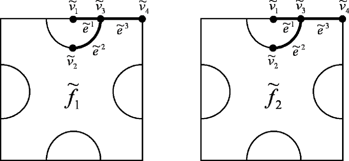
(a)

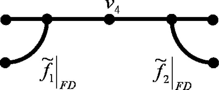
(b)

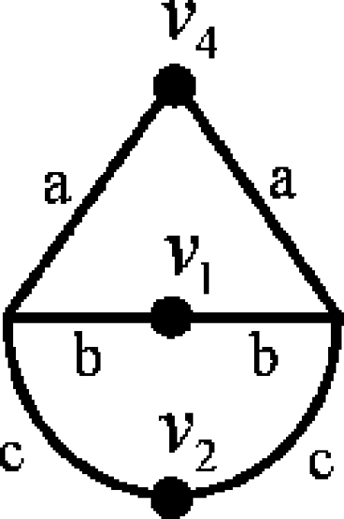
(c)

Figure 7: (a) Two copies of the graph $\Gamma$ which assist in the visualization of the functions $\tilde{f}_{1},\,\tilde{f}_{2}$ on $\Gamma$. The fundamental domain is marked in bold. (b) The first stage in the gluing process. The encoding is done by restricting $\tilde{f}_{1},\,\tilde{f}_{2}$ to the fundamental domain. (c) The quotient graph $\nicefrac{{\Gamma}}{{R}}$ which is built using the matrix representation (5.18). The boundary conditions are described in (5.27), (5.32).

We consider two functions $\tilde{f}_{1},\tilde{f}_{2}\in\Phi_{\Gamma}(\lambda)$ (for some $\lambda\in\mathbb{C}$) that transform according to the matrix representation (5.18). The first column of the matrix representing $\tau\sigma^{3}$ tells us that

$$\tau\sigma^{3}\tilde{f}_{1} = \,\tilde{f}_{1}-\nicefrac{{1}}{{2}}\,\tilde{f}_{2}$$ /32 (5.19)

$$\tau\sigma^{3}\tilde{f}_{1}^{\prime} = \,\tilde{f}_{1}^{\prime}-\nicefrac{{1}}{{2}}\,\tilde{f}_{2}^{\prime}$$ /32 (5.20)

Evaluating (5.19), (5.20) on $\tilde{v}_{4}$ and using the knowledge that $\tilde{f}_{1}$ obeys Neumann boundary conditions on $\tilde{v}_{4}$ (see equations (5.14), (5.15)) gives

$$\left(1-\nicefrac{{\sqrt{3}}}{{2}}\right)\,\tilde{f}_{1}\Big{|}_{\tilde{e}^{3}}(\tilde{v}_{4})+\nicefrac{{1}}{{2}}\,\tilde{f}_{2}\Big{|}_{\tilde{e}^{3}}(\tilde{v}_{4}) = 0\,.$$ (5.21)

$$\left(-1-\nicefrac{{\sqrt{3}}}{{2}}\right)\,\tilde{f}_{1}^{\prime}\Big{|}_{\tilde{e}^{3}}(\tilde{v}_{4})+\nicefrac{{1}}{{2}}\,\tilde{f}_{2}^{\prime}\Big{|}_{\tilde{e}^{3}}(\tilde{v}_{4}) = 0\,.$$ (5.22)

This indicates how we should start gluing the two subgraphs in order to obtain the quotient. The first stage in this process, depicted in figure 7(b), is to identify the vertex $\tilde{v}_{4}$ in the two copies and turn it into the vertex $v_{4}$ of the quotient, with the boundary conditions that were derived in (5.21), (5.22):

$$A_{v_{4}}=\left(\begin{array}[]{cc}1-\nicefrac{{\sqrt{3}}}{{2}}&\nicefrac{{1}}{{2}}\\ 0&0\end{array}\right) \quad,\quad B_{v_{4}}=\left(\begin{array}[]{cc}0&0\\ -1-\nicefrac{{\sqrt{3}}}{{2}}&\nicefrac{{1}}{{2}}\end{array}\right)\,.$$ (5.27)

After treating vertices $\tilde{v}_{1},\,\tilde{v}_{2}$ similarly we obtain the quotient $\nicefrac{{\Gamma}}{{R}}$ (figure 7(c)), whose remaining boundary conditions are given by:

$$A_{v_{1}}=A_{v_{2}}=\left(\begin{array}[]{cc}\nicefrac{{3}}{{2}}&\nicefrac{{\sqrt{3}}}{{2}}\\ 0&0\end{array}\right)\quad,\quad B_{v_{1}}=B_{v_{2}}=\left(\begin{array}[]{cc}0&0\\ -\nicefrac{{1}}{{2}}&\nicefrac{{\sqrt{3}}}{{2}}\end{array}\right)\,.$$ (5.32)

This last example demonstrates that for a multidimensional representation the quotient graph depends on the explicit matrix representation by which it is constructed. One choice of basis for the matrix representation gave us a quotient which is identical to one obtained previously (figure 2(a)), while another basis yielded a new quotient graph (figure 7(c)). As a matter of fact, all the examples of quotient graphs with respect to the various representations discussed so far (figures 2(a) and (b) and 5(b)) can also be obtained as quotients with respect to the representation $R$, by suitable choices of bases for its matrix representation. Furthermore, there are many other quantum graphs isospectral to these. For example, we consider an arbitrary orthogonal matrix representation of $R$, which is parameterized by :

$$\left\{\begin{array}[]{ccc}\tau\sigma^{2}&\mapsto&\left(\begin{array}[]{cc}\cos^{2}\theta-\sin^{2}\theta&-2\cos\theta\sin\theta\\ -2\cos\theta\sin\theta&-\cos^{2}\theta+\sin^{2}\theta\end{array}\right)\\ \\ \tau\sigma^{3}&\mapsto&\left(\begin{array}[]{cc}2\cos\theta\sin\theta&\cos^{2}\theta-\sin^{2}\theta\\ \cos^{2}\theta-\sin^{2}\theta&-2\cos\theta\sin\theta\end{array}\right)\end{array}\right\}$$

(e.g., (5.18) is obtained from $\theta=\nicefrac{{\pi}}{{3}}$). Using the general construction method, which is described in the next section, we obtain from this matrix representation the quotient given in figure 7(c), with the following boundary conditions:

$$A_{v_{1}}=A_{v_{2}}=\left(\begin{array}[]{cc}2\sin^{2}\theta&\sin 2\theta\\ \sin 2\theta&2-2\sin^{2}\theta\\ 0&0\\ 0&0\end{array}\right) A_{v_{4}}=\left(\begin{array}[]{cc}1-\sin 2\theta&2\sin^{2}\theta-1\\ 2\sin^{2}\theta-1&1+\sin 2\theta\\ 0&0\\ 0&0\end{array}\right)$$

$$B_{v_{1}}=B_{v_{2}}=\left(\begin{array}[]{cc}0&0\\ 0&0\\ 2-2\sin^{2}\theta&-\sin 2\theta\\ -\sin 2\theta&2\sin^{2}\theta\end{array}\right) B_{v_{4}}=\left(\begin{array}[]{cc}0&0\\ 0&0\\ 1+\sin 2\theta&1-2\sin^{2}\theta\\ 1-2\sin^{2}\theta&1-\sin 2\theta\end{array}\right).$$

The matrices above are not square ones as is required from the definition of the boundary conditions. However, since their role is to describe linear restrictions and due to the fact that they are all of rank one, they can be reduced to square matrices by deleting the appropriate rows. We thus get a continuous family of isospectral graphs. We already met some of its members. For example, $\theta=\nicefrac{{3\pi}}{{4}}$ gives the following boundary conditions:

$$A_{v_{1}}=A_{v_{2}}=\left(\begin{array}[]{cc}1&-1\\ 0&0\end{array}\right)\qquad \qquad A_{v_{4}}=\left(\begin{array}[]{cc}2&0\\ 0&0\end{array}\right)$$ (5.39)

$$B_{v_{1}}=B_{v_{2}}=\left(\begin{array}[]{cc}0&0\\ 1&1\end{array}\right)\qquad \qquad B_{v_{4}}=\left(\begin{array}[]{cc}0&0\\ 0&2\end{array}\right)$$ (5.44)

When applying this to figure 7(c), we notice that $v_{4}$ does not remain a vertex of degree two, but rather, splits into two vertices of degree one, one having Dirichlet boundary condition and the other Neumann. The vertices $v_{1}$ and $v_{2}$, however, stay connected and obtain Neumann boundary conditions. The resulting quotient is thus the one that we have already obtained as $\nicefrac{{\Gamma}}{{R_{2}}}$ (figure 2(b)). In a similar manner, the quotient $\nicefrac{{\Gamma}}{{R_{1}}}$ (figure 2(a)) is obtained from the choice $\theta=0$. We conclude by pointing out that the graph described in figure 7(c) is a good prototype for the isospectral family mentioned, yet it also might be misleading, since some members of the family have boundary conditions that tear apart the edges connected to some of the vertices, and thus change the connectivity of the graph. One should also pay attention to the fact that we have treated only orthogonal representations of $R$. We may further extend the isospectral family presented above by considering the broader case of all matrix representations of $R$. In particular, the quotient $\nicefrac{{\Gamma}}{{R_{3}}}$ (figure 5(b)) is obtained from the unitary representation

$$\left\{\begin{array}[]{cc}\sigma\mapsto\left(\begin{array}[]{cc}i&0\\ 0&-i\end{array}\right),&\tau\mapsto\left(\begin{array}[]{cc}0&-1\\ -1&0\end{array}\right)\end{array}\right\}\,.$$

6 The rigorous construction of a quotient graph

The rigorous formalism of the quotient graph construction is fully described and proven in [27]. Here we summarize this method in accordance with the discussion and demonstrations presented so far in this paper. Let $\Gamma$ be a quantum graph with a finite set of vertices $V$ and a finite set $E$ of edges connecting the vertices. Let $G$ be a finite group that acts on $\Gamma$, and $R$ a $d$-dimensional representation of $G$. We assume for now that $G$ acts freely on the edges, i.e., $ge\neq e$ for $e\in E$, $id\neq g\in G$, and leave the treatment of a non-free action on the edges for later (section 7.2). We may choose an ordered basis $B=\left(b_{j}\right)_{j=1}^{d}$ for $R$, with respect to which we think of it as a matrix representation. We choose representatives $\left\{\tilde{e}^{i}\right\}_{i=1}^{I}$ for the orbits $\nicefrac{{E}}{{G}}$, and likewise $\left\{\tilde{v}_{k}\right\}_{k=1}^{K}$ for $\nicefrac{{V}}{{G}}$. We shall assume, by adding “dummy” vertices (vertices of valency two with Neumann boundary conditions) if needed, that $G$ does not carry any vertex in $V$ to one of its neighbors. This ensures that no edge is transformed onto itself in the opposite direction, which would force us to take half the edge as a representative. The quotient graph $\nicefrac{{\Gamma}}{{R}}$ obtained from these choices is defined to have $\left\{v_{k}\right\}_{k=1}^{K}$ as its set of vertices, and $\left\{e_{j}^{i}\right\}_{j=1..d}^{i=1..I}$ for edges, where each $e_{j}^{i}$ is of length $l_{\tilde{e}^{i}}$. The vertices $v_{k}$, $v_{k^{\prime}}$ of $\nicefrac{{\Gamma}}{{R}}$ are connected by the edge $e_{j}^{i}$ if there exist $g,g^{\prime}\in G$ such that $\tilde{e}^{i}$ connects $g\tilde{v}_{k}$ to $g^{\prime}\tilde{v}_{k^{\prime}}$ in $\Gamma$. In such a case the vertices $v_{k}$, $v_{k^{\prime}}$ are connected by all the edges $\left\{e_{j}^{i}\right\}_{j=1}^{d}$. Until now we have used only the action of the group $G$ on $\Gamma$ in order to determine the edges and vertices of the quotient graph and its connectivity. Now we also need to use the information from $R$, $B$, and the boundary conditions of $\Gamma$, in order to specify the boundary conditions at each vertex $v_{k}$ in $\nicefrac{{\Gamma}}{{R}}$. Let the boundary conditions at $\tilde{v}_{k}$ in $\Gamma$ be described by $A_{\tilde{v}_{k}},\,B_{\tilde{v}_{k}}$. From here to the end of this section we focus on the vertex $v_{k}$ and its predecessor $\tilde{v}_{k}$, and keep in mind that our parameters depend on $k$ even when it is not reflected by the notations. The set of edges incident to the vertex $\tilde{v}_{k}$ can be written as $E_{\tilde{v}_{k}}=\left\{g_{l}\tilde{e}^{\nu_{l}}\right\}_{l=1}^{n}$, for some $\left\{g_{l}\right\}_{l=1}^{n}$ in G. Note that repetitions can occur among the $\nu_{l}$’s, and also among the $g_{l}$’s, and that their total number is $n=d_{\tilde{v}_{k}}$. The set of edges entering $v_{k}$ is $E_{v_{k}}=\left\{e_{j}^{\mu_{l^{\prime}}}\right\}_{{1\leq l^{\prime}\leq m\atop 1\leq j\leq d}}$, where $\left\{\mu_{l^{\prime}}\right\}_{l^{\prime}=1}^{m}$ is defined to be the set of distinct values among $\left\{\nu_{l}\right\}_{l=1}^{n}$. Obviously, $m\leq n$, and the relation between the sets $\left\{\mu_{l^{\prime}}\right\}_{l^{\prime}=1}^{m}$, $\left\{\nu_{l}\right\}_{l=1}^{n}$ is given by the $n\times m$ matrix

$$\Theta^{\prime}_{ll^{\prime}}=\left\{\begin{array}[]{ll}1&\mathchoice{\hbox{{$\displaystyle\nu_{l}=\mu_{l^{\prime}}$}}}{\hbox{{\firstchoice@false$\textstyle\nu_{l}=\mu_{l^{\prime}}$}}}{\hbox{{\firstchoice@false$\textstyle\nu_{l}=\mu_{l^{\prime}}$}}}{\hbox{{\firstchoice@false$\textstyle\nu_{l}=\mu_{l^{\prime}}$}}}\\ 0&\mathchoice{\hbox{{otherwise}}}{\hbox{{\firstchoice@false otherwise}}}{\hbox{{\firstchoice@false otherwise}}}{\hbox{{\firstchoice@false otherwise}}}\end{array}\right..$$

The resulting matrices (see [27]), describing the boundary conditions at $v_{k}$, are:

$$A_{v_{k}} = \left(A_{\tilde{v}_{k}}\otimes I_{d}\right)\cdot{\rm diag}\left(\left[\rho_{R}\left(g_{{1}}^{-1}\right)\right]_{B},\ldots,\left[\rho_{R}\left(g_{{n}}^{-1}\right)\right]_{B}\right)^{T}\cdot\left(\Theta^{\prime}\otimes I_{d}\right)$$ (6.1)

$$B_{v_{k}} = \left(B_{\tilde{v}_{k}}\otimes I_{d}\right)\cdot{\rm diag}\left(\left[\rho_{R}\left(g_{{1}}^{-1}\right)\right]_{B},\ldots,\left[\rho_{R}\left(g_{{n}}^{-1}\right)\right]_{B}\right)^{T}\cdot\left(\Theta^{\prime}\otimes I_{d}\right)\,.$$ (6.2)

Observe that the boundary conditions (6.1), (6.2) encapsulate the information of the boundary conditions on $\Gamma$ (given by $A_{\tilde{v}_{k}},B_{\tilde{v}_{k}}$), the action of the group ($\Theta^{\prime}$ and $\left\{g_{i}\right\}$), the representation ($\rho_{R}$) and the basis that was chosen for the representation ($B$). However, they may fail to be square matrices as our definition of a quantum graph calls for. We therefore need to discuss the question of how many linearly independent restrictions are dictated by those boundary conditions, i.e., find ${\rm rank}\left(A_{v_{k}}\,B_{v_{k}}\right)$. Let us assume that the original boundary conditions on $\tilde{v}_{k}$ were linearly independent, i.e. $\left(A_{\tilde{v}_{k}}\,B_{\tilde{v}_{k}}\right)$ is of maximal rank, $d_{\tilde{v}_{k}}$. If the action of $G$ is free not only on the edges but also on the vertices, then $\Theta^{\prime}$ is a permutation matrix and we get that $A_{v_{k}}$ and $B_{v_{k}}$ are square matrices. Furthermore, ${\rm rank}\left(A_{v_{k}}\,B_{v_{k}}\right)=d\cdot\mathrm{rank}\left(A_{\tilde{v}_{k}}\,B_{\tilde{v}_{k}}\right)=d\cdot d_{\tilde{v}_{k}}=d_{v_{k}}$, which means that $\left(A_{v_{k}}\,B_{v_{k}}\right)$ is also of maximal rank.

In the general case, it is shown in [27] that if the matrix $A_{\tilde{v}_{k}}\cdot B_{\tilde{v}_{k}}^{\dagger}$ is self-adjoint then ${\rm rank}\left(A_{v_{k}}\,B_{v_{k}}\right)=d_{v_{k}}$. This means that we may eliminate rows from $\left(A_{v_{k}}\,B_{v_{k}}\right)$, and remain with square $A_{v_{k}},\,B_{v_{k}}$ which still describe the same boundary conditions. Therefore, starting from a graph $\Gamma$ whose Laplacian is self-adjoint, any $\nicefrac{{\Gamma}}{{R}}$ produced by this construction method would be a valid quantum graph (whether the Laplacian on $\nicefrac{{\Gamma}}{{R}}$ is also self-adjoint is discussed in section 7.3). This also demonstrates the benefits of using quantum graphs to implement the quotient construction. Although one may apply the above procedure to other types of objects (see section 9), the resulting quotients might not be objects of the same type as their predecessors. The advantage of quantum graphs in this context is that the self-adjointness condition guarantees that the quotient is a quantum graph as well.

We now recall the intimate relation between the construction of $\nicefrac{{\Gamma}}{{R}}$ and the encoding process, which for each $\lambda\in\mathbb{C}$ takes functions $\widetilde{f}_{1},\ldots,\widetilde{f}_{d}\in\Phi_{\Gamma}(\lambda)$ that transform according to $R$, and maps them to a single function $f\in\Phi_{\nicefrac{{\Gamma}}{{R}}}(\lambda)$. This encoding is described by:

$$f\Big{|}_{e_{j}^{i}} \equiv \widetilde{f}_{j}\Big{|}_{\tilde{e}^{i}}.$$ (6.3)

This relation gives the decoding process as well $-$ starting from $f\in\Phi_{\nicefrac{{\Gamma}}{{R}}}(\lambda)$, one reconstructs the values of $\tilde{f}_{1},\ldots,\tilde{f}_{d}\in\Phi_{\Gamma}(\lambda)$ on the edges’ representatives $\left\{{\tilde{e}^{i}}\right\}$. The values on the rest of the edges are then determined by the action of $G$ and the representation $R$.

We elaborate on the functions $\tilde{f}_{1},\ldots,\tilde{f}_{d}\in\Phi_{\Gamma}(\lambda)$ that play a role in the decoding-encoding process. For two representations $R,R^{\prime}$ with corresponding carrier spaces $V,V^{\prime}$, ${\rm Hom}_{G}\left(V,V^{\prime}\right)$ is the vector space of all linear transformations $T:V\rightarrow V^{\prime}$ that respect the action of the group $G$, i.e., $\forall g\in G,v\in V:\;T(\rho_{R}(g)\,v)=\rho_{R^{\prime}}(g)\,T(v)$. Such linear transformations are called intertwiners of the representations $R,\,R^{\prime}$. It is known that $\left\langle\chi_{R},\chi_{\Phi_{\Gamma}\left(\lambda\right)}\right\rangle_{G}=\dim{\rm Hom}_{G}\left(R,\Phi_{\Gamma}\left(\lambda\right)\right)$ ([38], section 9C) and we recall that the quotient graph’s construction guarantees $\sigma_{\nicefrac{{\Gamma}}{{R}}}(\lambda)=\left\langle\chi_{R},\chi_{\Phi_{\Gamma}\left(\lambda\right)}\right\rangle_{G}$. We therefore have that $\Phi_{\nicefrac{{\Gamma}}{{R}}}(\lambda)\cong{\rm Hom}_{G}\left(R,\Phi_{\Gamma}\left(\lambda\right)\right)$, which offers another point of view on our quotient graphs. We demonstrate this by an example. Let $G$ be a group and $R=S\oplus S\oplus S$, for some irreducible representation $S$ of $G$, and let $\lambda\in\mathbb{C}$ be such that $\Phi_{\Gamma}(\lambda)\cong V_{1}^{S}\oplus V_{2}^{S}$, where $V_{1}^{S},\,V_{2}^{S}$ are carrier spaces of $S$. Since $\dim{\rm Hom}_{G}\left(R,\Phi_{\Gamma}\left(\lambda\right)\right)=\left\langle\chi_{R},\chi_{\Phi_{\Gamma}\left(\lambda\right)}\right\rangle_{G}=\left\langle 3\chi_{S},2\chi_{S}\right\rangle_{G}=6$, we can choose six linearly independent intertwiners from $V^{R}$ to $\Phi_{\Gamma}\left(\lambda\right)$. One such choice of intertwiners can be described as follows. We decompose a carrier space of $R$, $V^{R}$, into three carrier spaces of $S$ and each intertwiner then sends one of these three copies onto either $V_{1}^{S}$ or $V_{2}^{S}$, and the other two copies to zero.
The quotient $\nicefrac{{\Gamma}}{{R}}$ is constructed with respect to a certain basis $B$ of $R$. The image of this basis by each of the above six intertwiners is a set of $d={\rm dim}\,R$ functions, $\tilde{f}_{1},\ldots,\tilde{f}_{d}\in\Phi_{\Gamma}(\lambda)$ which transform according to $R$ , and this set can be encoded by a function $f\in\Phi_{\nicefrac{{\Gamma}}{{R}}}(\lambda)$ according to (6.3). We thus obtain six linearly independent eigenfunctions of the eigenvalue $\lambda$ on the quotient $\nicefrac{{\Gamma}}{{R}}$, which demonstrates the equivalence $\Phi_{\nicefrac{{\Gamma}}{{R}}}(\lambda)\cong{\rm Hom}_{G}\left(R,\Phi_{\Gamma}\left(\lambda\right)\right)$.

7 Application of the method $-$ Further investigation

Having revealed the key elements of the construction method, we are ready to present its theoretical implications, as well as various issues that may interest those who wish to apply it.

7.1 Sunada’s isospectral theorem

In his famous paper [2], Sunada provides a method for producing isospectral Riemannian manifolds. Phrasing his result somewhat loosely, given a manifold $M$ equipped with a free action of a finite group $G$, and subgroups $H_{1},\,H_{2}$ of $G$ which are almost conjugate, the manifolds $\nicefrac{{M}}{{H_{1}}}$ and $\nicefrac{{M}}{{H_{2}}}$ are isospectral. $H_{1}$ and $H_{2}$ are said to be almost conjugate if $\,\,\forall g\in G\quad|\{[g]\cap H_{1}\}|=|\{[g]\cap H_{2}\}|$, where $[g]$ denotes the conjugacy class of $g$ in G. As mentioned and proved in [5], $H_{1}$ and $H_{2}$ are almost conjugate iff ${\rm Ind}_{H_{1}}^{G}\mathbf{1}_{H_{1}}\cong{\rm Ind}_{H_{2}}^{G}\mathbf{1}_{H_{2}}$, where $\mathbf{1}_{H_{i}}$ is the trivial representation of $H_{i}$. Comparing this to corollary 4.4, we see that Sunada’s theorem is obtained as a particular case of the corollary if $\nicefrac{{M}}{{H_{i}}}$ is isospectral to $\nicefrac{{M}}{{\mathbf{1}_{H_{i}}}}$. This is indeed the case since the space of functions on $\nicefrac{{M}}{{H_{i}}}$ is isomorphic to the space of functions on $M$ which are invariant under the action of $H_{i}$. But the latter is the trivial component of the space of functions on $M$, which by definition is isomorphic to the space of functions on $\nicefrac{{M}}{{\mathbf{1}_{H_{i}}}}$, so that

$$\forall\lambda\in\mathbb{C}\quad\Phi_{\nicefrac{{M}}{{H_{i}}}}(\lambda)\cong\Phi_{M}^{\mathbf{1}_{H_{i}}}(\lambda)\cong\Phi_{\nicefrac{{M}}{{\mathbf{1}_{H_{i}}}}}(\lambda),$$

as claimed. During the discussion above we have applied our isospectral theory to manifolds, as opposed to quantum graphs, for which it was developed in the previous sections. This should not bother us - the method can be applied to other geometric objects, as will be demonstrated in section 9. Finally, we note that the equivalence of ${\rm Ind}_{H_{1}}^{G}\mathbf{1}_{H_{1}}\cong{\rm Ind}_{H_{2}}^{G}\mathbf{1}_{H_{2}}$ and $H_{1},H_{2}$ being almost conjugate was already used by Pesce [28] to give another proof for Sunada’s theorem. Our application of Frobenius Reciprocity for the proof of theorem 4.3 is similar to that of Pesce, whose proof is also summarized comprehensibly in [5].

7.2 A non-free action on the edges

We now treat the case of a group whose action on the edges is not free. We have already encountered examples of non-free action on the vertices, and saw that this may result in the vertex in the quotient graph having a degree smaller than that of its predecessor. An action which is not free on the edges results in some more interesting features. Denote by $\Gamma$ the quantum graph which is an equilateral tetrahedron equipped with Neumann boundary conditions at all its vertices (figure 8).

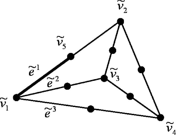
Figure 8: An equilateral tetrahedron with Neumann boundary conditions. It is equipped with an action of $S_{4}$ permuting its vertices $\tilde{v}_{1},\,\tilde{v}_{2},\,\tilde{v}_{3},\,\tilde{v}_{4}$.

Note that we have added “dummy” vertices in the middle of the edges, as described in the previous section. $S_{4}$ acts by permuting the vertices $\tilde{v}_{1},\,\tilde{v}_{2},\,\tilde{v}_{3},\,\tilde{v}_{4}$, and this determines its action on the whole of $\Gamma$. Let $S$ denote the sign representation of $S_{4}$:

$$\forall\sigma\in S_{4}\quad\rho_{S}\left(\sigma\right)=\left(\mathrm{sgn}\,\sigma\right)\,.$$ (7.1)

We choose the edge $\tilde{e}^{1}$ and the vertices $\tilde{v}_{1},\,\tilde{v}_{5}$ as a fundamental domain for the action of $S_{4}$. A function $\tilde{f}$ which transforms according to $S$ satisfies $(3\,4)\,\tilde{f}=\rho_{S}\left[(3\,4)\right]\tilde{f}=-\tilde{f}$. Evaluating this on the edge $\tilde{e}^{1}$ gives $\tilde{f}\Big{|}_{\tilde{e}^{1}}=\tilde{f}\Big{|}_{(3\,4)\tilde{e}^{1}}=\left((3\,4)\tilde{f}\right)\Big{|}_{\tilde{e}^{1}}=-\tilde{f}\Big{|}_{\tilde{e}^{1}}$, which means that $\tilde{f}$ vanishes on $\tilde{e}^{1}$ and therefore also on the whole of $\Gamma$. We conclude that $\Gamma$’s Laplacian has no eigenfunctions which transform according to $S$, so that $\nicefrac{{\Gamma}}{{S}}$ is just the empty graph. Putting this another way, the edge $\tilde{e}^{1}$ of $\Gamma$ was chosen as a representative for the orbits of the edges under the action of the group, $\nicefrac{{E}}{{S_{4}}}$. We therefore expected to have a single edge $e_{1}^{1}$ in the quotient. However, this edge has disappeared due to the action of the stabilizer of $\tilde{e}^{1}$. Specifically, the stabilizer is $G_{\tilde{e}^{1}}=\left\{id,(3\,4)\right\}$ and the restriction of the representation on it is not trivial: $\rho_{S}\Big{|}_{G_{\tilde{e}^{1}}}\neq 1$. This caused the disappearance.

Moving to a more complex demonstration of this principle, we examine the permutation representation of $S_{4}$, which we denote by $R$. Some of the matrices of $R$ using its standard basis are:

$$\left\{\begin{array}[]{ll}(1\,2)\mapsto\scriptsize{\left(\begin{array}[]{cccc}0&1&0&0\\ 1&0&0&0\\ 0&0&1&0\\ 0&0&0&1\end{array}\right)},&(3\,4)\mapsto\scriptsize{\left(\begin{array}[]{cccc}1&0&0&0\\ 0&1&0&0\\ 0&0&0&1\\ 0&0&1&0\end{array}\right)}\\ \\ (2\,3\,4)\mapsto\scriptsize{\left(\begin{array}[]{cccc}1&0&0&0\\ 0&0&0&1\\ 0&1&0&0\\ 0&0&1&0\end{array}\right)},&(2\,4\,3)\mapsto\scriptsize{\left(\begin{array}[]{cccc}1&0&0&0\\ 0&0&1&0\\ 0&0&0&1\\ 0&1&0&0\end{array}\right)}\end{array}\right\}.$$ (7.2)

We choose the same fundamental domain and consider the values of the functions $\tilde{f}_{1},\tilde{f}_{2},\tilde{f}_{3},\tilde{f}_{4}$ (which transform according to (7.2)) on it. We now have four edges, $e^{1}_{1},e^{1}_{2},e^{1}_{3},e^{1}_{4}$, that are supposed to form the quotient graph after we properly glue them and deduce the boundary conditions. From the action of $(2\,3\,4)$ and $(2\,4\,3)$ on $\tilde{f}_{1}$, the chosen matrix representation for $R$, and the fact that $\tilde{v}_{1}$ has Neumann boundary conditions, it follows that $\tilde{f}_{1}^{\prime}\Big{|}_{\tilde{e}^{1}}(\tilde{v}_{1})=0$. Likewise, from the action of $(1\,2)$ on $\tilde{f}_{1}$ we conclude that $\tilde{f}_{1}\Big{|}_{\tilde{e}^{1}}(\tilde{v}_{5})=\tilde{f}_{2}\Big{|}_{\tilde{e}^{1}}(\tilde{v}_{5})$ and $\tilde{f}_{1}^{\prime}\Big{|}_{\tilde{e}^{1}}(\tilde{v}_{5})+\tilde{f}_{2}^{\prime}\Big{|}_{\tilde{e}^{1}}(\tilde{v}_{5})=0$ (where the derivatives are outgoing from $\tilde{v}_{5}$). This allows us glue the edges $e_{1}^{1},\,e_{2}^{1}$ and deduce a Neumann condition on the left side of $e_{1}^{1}$ (figure 9). These considerations are similar to those used before, and the new part comes when we observe that $(3\,4)\tilde{f}_{3}=\tilde{f}_{4}$. This gives $\tilde{f}_{3}\Big{|}_{\tilde{e}^{1}}=\tilde{f}_{4}\Big{|}_{\tilde{e}^{1}}$ and means that we do not need both of the corresponding edges (i.e., $e_{3}^{1}$ and $e_{4}^{1}$) in the quotient graph . We notice that the problem arises since the representation restricted to the stabilizer $G_{\tilde{e}^{1}}=\left\{id,(3\,4)\right\}$ has a non trivial component ($\rho_{R}\left[(3\,4)\right]$ has an eigenvalue not equal to one). The solution for this situation is to change our basis in the following way:

$$\begin{array}[]{ll}\hat{f}_{1}=\tilde{f}_{1},&\hat{f}_{3}=\frac{1}{\sqrt{2}}\left(\tilde{f}_{3}+\tilde{f}_{4}\right)\\ \hat{f}_{2}=\tilde{f}_{2},&\hat{f}_{4}=\frac{1}{\sqrt{2}}\left(\tilde{f}_{3}-\tilde{f}_{4}\right)\,,\end{array}$$

This forces us to rewrite (7.2) as

$$\left\{\begin{array}[]{ll}(1\,2)\mapsto\scriptsize{\left(\begin{array}[]{cccc}0&1&0&0\\ 1&0&0&0\\ 0&0&1&0\\ 0&0&0&1\end{array}\right)},&(3\,4)\mapsto\scriptsize{\left(\begin{array}[]{cccc}1&0&0&0\\ 0&1&0&0\\ 0&0&1&0\\ 0&0&0&-1\end{array}\right)}\\ \\ (2\,3\,4)\mapsto\scriptsize{\left(\begin{array}[]{cccc}1&0&0&0\\ 0&0&\nicefrac{{1}}{{\sqrt{2}}}&-\nicefrac{{1}}{{\sqrt{2}}}\\ 0&\nicefrac{{1}}{{\sqrt{2}}}&\nicefrac{{1}}{{2}}&\nicefrac{{1}}{{2}}\\ 0&\nicefrac{{1}}{{\sqrt{2}}}&-\nicefrac{{1}}{{2}}&-\nicefrac{{1}}{{2}}\end{array}\right)},&(2\,4\,3)\mapsto\scriptsize{\left(\begin{array}[]{cccc}1&0&0&0\\ 0&0&\nicefrac{{1}}{{\sqrt{2}}}&\nicefrac{{1}}{{\sqrt{2}}}\\ 0&\nicefrac{{1}}{{\sqrt{2}}}&\nicefrac{{1}}{{2}}&-\nicefrac{{1}}{{2}}\\ 0&-\nicefrac{{1}}{{\sqrt{2}}}&\nicefrac{{1}}{{2}}&-\nicefrac{{1}}{{2}}\end{array}\right)}\end{array}\right\}.$$ (7.3)

Examining the action of $(3\,4)$ on $\hat{f}_{4}$, we get $\hat{f}_{4}\Big{|}_{\tilde{e}^{1}}\equiv 0$ and this turns out to be the edge which disappears. The previous considerations we made concerning $\tilde{f}_{1}\Big{|}_{\tilde{e}^{1}}$ and $\tilde{f}_{2}\Big{|}_{\tilde{e}^{1}}$ are still valid since $\hat{f}_{1}=\tilde{f}_{1},\,\hat{f}_{2}=\tilde{f}_{2}$. The last step in the gluing process follows from the second column of the matrix representations of $(2\,3\,4),\,(2\,4\,3)$, and the evaluation of the corresponding relations on $\tilde{e}^{1}$:

$$\hat{f}_{2}\Big{|}_{\tilde{e}^{3}}= \left((2\,3\,4)\,\hat{f}_{2}\right)\Big{|}_{\tilde{e}^{1}} =\nicefrac{{1}}{{\sqrt{2}}}\,\hat{f}_{3}\Big{|}_{\tilde{e}^{1}}+\nicefrac{{1}}{{\sqrt{2}}}\,\hat{f}_{4}\Big{|}_{\tilde{e}^{1}}$$ (7.4)

$$\hat{f}_{2}\Big{|}_{\tilde{e}^{2}}= \left((2\,4\,3)\,\hat{f}_{2}\right)\Big{|}_{\tilde{e}^{1}} =\nicefrac{{1}}{{\sqrt{2}}}\,\hat{f}_{3}\Big{|}_{\tilde{e}^{1}}-\nicefrac{{1}}{{\sqrt{2}}}\,\hat{f}_{4}\Big{|}_{\tilde{e}^{1}}$$ (7.5)

Recalling that $\hat{f}_{4}\Big{|}_{\tilde{e}^{1}}\equiv 0$ and using (7.4), (7.5) to obtain relations for the derivatives as well, we finish the process and give the quotient $\nicefrac{{\Gamma}}{{S}}$ that is shown in figure 9.

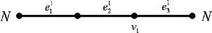
$A_{v_{1}}=\scriptsize{\left(\begin{array}[]{cc}\sqrt{2}&-1\\ 0&0\end{array}\right)}$

$B_{v_{1}}=\scriptsize{\left(\begin{array}[]{cc}0&0\\ 1&\sqrt{2}\end{array}\right)}$

Figure 9: The quotient $\nicefrac{{\Gamma}}{{S}}$. The only non-Neumann boundary condition is at $v_{1}$ and it is specified by the matrices $A_{v_{1}},B_{v_{1}}$.

We now return to the general construction procedure described in the previous section, and discuss the adjustments that should be made in order to apply it to the case of a non-free action on the edges. After choosing the representatives $\left\{\tilde{e}^{i}\right\}_{i=1}^{I}$ for the orbits $\nicefrac{{E}}{{G}}$, we consider for each $i$ the representation ${\rm Res}_{G_{\tilde{e}^{i}}}^{G}S$ with its carrier space $V^{i}$. We decompose $V^{i}$ into its trivial component, $\left(V^{i}\right)^{\mathbf{1}_{G_{\tilde{e}^{i}}}}$, and its complement, $\bigoplus\limits_{S\ncong\mathbf{1}_{G_{\tilde{e}^{i}}}}\left(V^{i}\right)^{S}$. We denote the dimension of the trivial component of $V^{i}$ by $d_{i}$ and choose a basis for it: $\left\{b_{j}^{i}\right\}_{j=1}^{d_{i}}$. We complete this to a basis for the whole of $V^{i}$ by adding vectors from the complement of $\left(V^{i}\right)^{\mathbf{1}_{G_{\tilde{e}^{i}}}}$, and we denote this basis, $\left\{b_{j}^{i}\right\}_{j=1}^{d}$, by $B^{i}$. Let $\left\{\widetilde{f}^{i}_{j}\Big{|}_{\tilde{e}^{i}}\right\}_{j=1}^{d}$ be functions on the edge $\tilde{e}^{i}$ which transform according to the representation $R$ as given by the basis $B^{i}$. As in the preceding examples we have that $\forall j>d_{i},\;\;\widetilde{f}^{i}_{j}\Big{|}_{\tilde{e}^{i}}=0$ . Therefore, in the assembly of the quotient, we endow it with only $d_{i}$ copies of the edge $\tilde{e}^{i}$ $-$ the copies which correspond to the functions $\left\{\widetilde{f}^{i}_{j}\Big{|}_{\tilde{e}^{i}}\right\}_{j=1}^{d_{i}}$. Equations (6.1), (6.2) are replaced in the general case by the following:

$$A_{v_{k}} = \left(A_{\tilde{v}_{k}}\otimes I_{d}\right)\cdot{\rm diag}\left(\left[\rho_{R}\left(g_{{1}}^{-1}\right)\right]_{B^{\nu_{1}}}^{B},\ldots,\left[\rho_{R}\left(g_{{n}}^{-1}\right)\right]_{B^{\nu_{n}}}^{B}\right)^{T}\cdot\Theta$$ (7.6)

$$B_{v_{k}} = \left(B_{\tilde{v}_{k}}\otimes I_{d}\right)\cdot{\rm diag}\left(\left[\rho_{R}\left(g_{{1}}^{-1}\right)\right]_{B^{\nu_{1}}}^{B},\ldots,\left[\rho_{R}\left(g_{{n}}^{-1}\right)\right]_{B^{\nu_{n}}}^{B}\right)^{T}\cdot\Theta$$ (7.7)

One obvious difference is the use of a separate basis $B^{i}$ for each edge that enters the vertex. The other change is due to $\Theta$ which is defined to be the $nd\times d_{v_{k}}$ matrix obtained by removing from $\left(\Theta^{\prime}\otimes I_{d}\right)$ the columns $\left\{\left(i-1\right)\cdot d+j\right\}_{{1\leq i\leq m\atop d_{\mu_{i}}<j\leq d}}$; these are the columns which represent the functions whose vanishing on the corresponding edge ($\tilde{e}^{i}$) of the graph $\Gamma$ causes the disappearance of ($d-d_{i}$) copies of that edge from the quotient. Note that (6.1), (6.2) are obtained as a special case of (7.6), (7.7) when the action is free on the edges and a single choice of basis is made (i.e., $B^{1}=\ldots=B^{I}=B$). In addition, the encoding$\setminus$decoding process in this case is then slightly altered from the one described by (6.3). For each $\lambda\in\mathbb{C}$ and $1\leq i\leq I$, a set of functions $\widetilde{f}^{i}_{1},\ldots,\widetilde{f}^{i}_{d}\in\Phi_{\Gamma}(\lambda)$ that transform according to the basis $B^{i}$ of $R$ is mapped into a single function $f\in\Phi_{\nicefrac{{\Gamma}}{{R}}}(\lambda)$ by:

$$\forall 1\leq j\leq d_{i},\;\;f\Big{|}_{e_{j}^{i}} \equiv \widetilde{f}^{i}_{j}\Big{|}_{\tilde{e}^{i}}.$$ (7.8)

Note that the functions $\left\{\widetilde{f}^{i}_{j}\Big{|}_{\tilde{e}^{i}}\right\}_{1\leq i\leq I\atop{d_{i}<j\leq d}}$ are zero and therefore not encoded. Finally, the discussion that comes after equations (6.1), (6.2) regarding the rank of $A_{v_{k}}B_{v_{k}}$ is valid here as well: whenever the Laplacian on $\Gamma$ is self-adjoint, the produced quotient obeys the definition of a quantum graph.

7.3 The self-adjointness of the Laplacian on the quotient graph

A natural question to ask is whether the Laplacian on the quotient graph produced by the above construction is self-adjoint. The necessary and sufficient conditions for the self-adjointness of a quantum graph were described in section 2. Their examination in light of (7.6), (7.7) gives the following:

Proposition 7.1.

Let $\nicefrac{{\Gamma}}{{R}}$ be a quotient quantum graph constructed as explained in section (7.2).

1. If $\Gamma$’s Laplacian is self-adjoint, $G$ acts freely on $\Gamma$ (both on the edges and the vertices), and $\left[\rho_{R}\left(g\right)\right]_{B}^{B^{i}}$ is unitary for all $g\in G$, $1\leq i\leq I$, then the Laplacian on $\nicefrac{{\Gamma}}{{R}}$ is self-adjoint.

2. If $\Gamma$ has Neumann boundary conditions and $\left[\rho_{R}\left(g\right)\right]_{B}^{B^{i}}$ is unitary for all $g,i$, then the Laplacian on $\nicefrac{{\Gamma}}{{R}}$ is self-adjoint if and only if for every vertex $\tilde{v}$ at least one of the following holds:

   1. $\left\langle\chi_{R},\mathbf{1}\right\rangle_{G_{\tilde{v}}}=0$.

   2. All stabilizers $\left\{G_{\tilde{e}}\right\}_{\tilde{e}\in E_{\tilde{v}}}$ are of equal order.

Remark.

Since $G$ is assumed to be finite, one dimensional representations are unitary in all bases.

Proof.

We start by recalling the observations made in sections 6, 7.2. When $\Gamma$ has a self-adjoint Laplacian, our construction ensures that for every vertex $v$ of the quotient we have ${\rm rank}\left(A_{v}\,B_{v}\right)=d_{v}$. Therefore, one condition required for the self-adjointness of the quotient is fulfilled, and we are left to verify the other, $A_{v}\cdot B_{v}^{\dagger}=B_{v}\cdot A_{v}^{\dagger}$.

1. Let $\tilde{v}$ be a vertex in $\Gamma$, with $E_{\tilde{v}}=\left\{g_{i}\tilde{e}^{\nu_{i}}\right\}_{i=1}^{n}$, and $v$ the corresponding vertex in $\nicefrac{{\Gamma}}{{R}}$. Since the action is free both on the edges and on the vertices we have $\Theta^{\prime}=I_{n}$ (by appropriate indexing of the edges) and $\Theta=\Theta^{\prime}\otimes I_{d}=I_{d_{v}}$ (since the free action also implies $d_{v}=d_{\tilde{v}}\cdot d=n\cdot d$). The unitarity of the representation with respect to the bases $B^{i}$ and $B$ gives that $D:={\rm diag}\left(\left[\rho_{R}\left(g_{{1}}^{-1}\right)\right]^{B}_{B^{\nu_{1}}},\ldots,\left[\rho_{R}\left(g_{{n}}^{-1}\right)\right]^{B}_{B^{\nu_{n}}}\right)^{T}$ is a unitary matrix. Therefore,

   $$A_{v}\cdot B_{v}^{\dagger} = \left(A_{\tilde{v}}\otimes I_{d}\right)\cdot D\cdot I_{d_{v}}\cdot\left(\left(B_{\tilde{v}}\otimes I_{d}\right)\cdot D\cdot I_{d_{v}}\right)^{\dagger}$$

   $$= \left(A_{\tilde{v}}\otimes I_{d}\right)\cdot\left(B_{\tilde{v}}\otimes I_{d}\right)^{\dagger}=\left(A_{\tilde{v}}\cdot B_{\tilde{v}}^{\dagger}\right)\otimes I_{d}$$

   $$= \left(B_{\tilde{v}}\cdot A_{\tilde{v}}^{\dagger}\right)\otimes I_{d}=B_{v}\cdot A_{v}^{\dagger}\,\,.$$

2. Let $v$ be a vertex of $\nicefrac{{\Gamma}}{{R}}$, and $\tilde{v}$ its predecessor in $\Gamma$. Recall (section 6) that $E_{\tilde{v}}=\left\{g_{i}\tilde{e}^{\nu_{i}}\right\}_{i=1}^{n}$, and that $\left\{\nu_{i}\right\}_{i=1}^{n}$ attain in total $m$ distinct values, $\left\{\mu_{i}\right\}_{i=1}^{m}$. We assume (by reordering, if necessary) that $\left\{\nu_{i}\right\}_{i=1}^{m}$ are different: this means that $\left\{g_{i}\tilde{e}^{\nu_{i}}\right\}_{i=1}^{m}$ are representatives for the different orbits of the edges in $E_{\tilde{v}}.$ For each $1\leq i\leq m$ we choose a set of representatives $\left\{t_{i}^{j}\right\}_{j=1}^{r_{i}}$ ($r_{i}=\left[G_{\tilde{v}}:G_{g_{i}\tilde{e}^{\nu_{i}}}\right]$) for the left cosets of $G_{g_{i}\tilde{e}^{\nu_{i}}}$ in $G_{\tilde{v}}$, so that when writing $E_{\tilde{v}}=\left\{t_{i}^{j}g_{i}\tilde{e}^{\nu_{i}}\right\}_{{i=1..m\atop j=1..r_{i}}}$ we obtain each edge in $E_{\tilde{v}}$ exactly once. This is the ordering with which we represent the boundary conditions at $\tilde{v}$.

   Denoting

   $$\mathfrak{g}_{i,j}=\left(\left[\rho_{R}\left(t_{i}^{j}g_{i}\right)^{-1}\right]_{B^{\nu_{i}}}^{B}\right)^{T}\,,\qquad\theta_{i}=\left(\begin{array}[]{c|c}I_{d_{\nu^{i}}}&\vphantom{I_{d_{\nu^{i}}}}0\\ \hline\cr\vphantom{I_{d_{\nu^{i}}}}0&\vphantom{I_{d_{\nu^{i}}}}0\end{array}\right)\,\in\,M_{d\times d}\left(\mathbb{C}\right)\>,$$

   $$\mathfrak{G}=\mathrm{diag}\left(\mathfrak{g}_{1,1},\ldots,\mathfrak{g}_{1,r_{1}},\mathfrak{g}_{2,1},\ldots\ldots,\mathfrak{g}_{m,r_{m}}\right),$$

   we have

   $$\mathfrak{G}\Theta\Theta^{\dagger}\mathfrak{G}^{\dagger}=\scriptsize\left(\begin{array}[]{ccccccc}\mathfrak{g}_{1,1}\theta_{1}\mathfrak{g}_{1,1}^{\dagger}&\cdots&\mathfrak{g}_{1,1}\theta_{1}\mathfrak{g}_{1,r_{1}}^{\dagger}&&&&\\ \vdots&\ddots&\vdots&&&&\\ \mathfrak{g}_{1,r_{1}}\theta_{1}\mathfrak{g}_{1,1}^{\dagger}&\cdots&\mathfrak{g}_{1,r_{1}}\theta_{1}\mathfrak{g}_{1,r_{1}}^{\dagger}&&&&\\ &&&\ddots&&&\\ &&&&\mathfrak{g}_{m,1}\theta_{m}\mathfrak{g}_{m,1}^{\dagger}&\cdots&\mathfrak{g}_{m,1}\theta_{m}\mathfrak{g}_{m,r_{m}}^{\dagger}\\ &&&&\vdots&\ddots&\vdots\\ &&&&\mathfrak{g}_{m,r_{m}}\theta_{m}\mathfrak{g}_{m,1}^{\dagger}&\cdots&\mathfrak{g}_{m,r_{m}}\theta_{m}\mathfrak{g}_{m,r_{m}}^{\dagger}\end{array}\right)\>.$$

   The Neumann boundary conditions at $\tilde{v}$ can be expressed by

   $$A_{\tilde{v}}=\scriptsize{\left(\begin{array}[]{cccc}1&-1\\ \vdots&&\ddots\\ 1&&&-1\\ 0&\cdots&0&0\end{array}\right)}\qquad B_{\tilde{v}}=\scriptsize{\left(\begin{array}[]{cccc}0&0&\cdots&0\\ \vdots&\vdots&\ddots&\vdots\\ 0&0&\cdots&0\\ 1&1&\cdots&1\end{array}\right)}\,$$

   and using (7.6), (7.7) we have $B_{v}A_{v}^{\dagger}=\left(B_{\tilde{v}}\otimes I_{d}\right)\mathfrak{G}\Theta\Theta^{\dagger}\mathfrak{G}^{\dagger}\left(A_{\tilde{v}}\otimes I_{d}\right)^{\dagger}$ and can write $B_{v}A_{v}^{\dagger}$ in $d\times d$ blocks:

   $$B_{v}A_{v}^{\dagger}=\scriptsize\left(\begin{array}[]{cccccccc}\left[0\right]&\cdots&\left[0\right]&\left[0\right]&\cdots&\cdots&\left[0\right]&\left[0\right]\\ \vdots&&\vdots&\vdots&&&\vdots&\vdots\\ \left[0\right]&\cdots&\left[0\right]&\left[0\right]&\cdots&\cdots&\left[0\right]&\left[0\right]\\ \left[M_{1,1}-M_{1,2}\right]&\cdots&\left[M_{1,1}-M_{1,r_{1}}\right]&\left[M_{1,1}-M_{2,1}\right]&\cdots&\cdots&\left[M_{1,1}-M_{m,r_{m}}\right]&\left[0\right]\end{array}\right),$$

   where for $1\leq i\leq m$,   $1\leq j\leq r_{i}$ we denote

   $$M_{i,j}=\sum_{k=1}^{r_{i}}\mathfrak{g}_{i,k}\theta_{i}\mathfrak{g}_{i,j}^{\dagger}.$$

   Due to the fact that $B_{v}A_{v}^{\dagger}$ is strictly lower-triangular, it can only be self-adjoint if it is zero, i.e., if $M_{i,j}$ is the same for all $i,j$, and we wish to analyze when this occurs. First, we note that

   $$\theta_{i}=\frac{1}{\left|G_{\tilde{e}^{\nu_{i}}}\right|}\sum\limits_{g\in G_{\tilde{e}^{\nu_{i}}}}\left[\rho_{R}\left(g\right)\right]_{B^{\nu_{i}}}^{B^{\nu_{i}}}\>,$$ (7.10)

   by the following observations:
   (a) For every irreducible representation $\rho_{S}$ of a group $G$ we have

   $$\frac{1}{\left|G\right|}\sum\limits_{g\in G}\rho_{S}\left(g\right)=\left\{\begin{array}[]{ccc}I&&S\cong\mathbf{1}_{G}\\ 0&&S\ncong\mathbf{1}_{G}\end{array}\right.$$ (7.11)

   (b) As explained in section 7.2, we chose $B^{\nu_{i}}=\left\{b_{j}^{\nu_{i}}\right\}_{j=1}^{d}$ such that $\left\{b_{j}^{\nu_{i}}\right\}_{j=1}^{d_{\nu_{i}}}$ is a basis for the trivial component of ${\rm Res}^{G}_{G_{\tilde{e}^{\nu_{i}}}}R$, and $\left\{b_{j}^{\nu_{i}}\right\}_{j=d_{\nu_{i}}+1}^{d}$ is a basis for $\bigoplus\limits_{S\ncong\mathbf{1}_{G}}\left(\mathrm{Res}_{G_{\tilde{e}^{\nu_{i}}}}^{G}R\right)^{S}$.
   
   By our unitarity assumption, $\left(\left[\rho_{R}\left(t_{i}^{j}g_{i}\right)^{-1}\right]_{B^{\nu_{i}}}^{B}\right)^{\dagger}=\left[\rho_{R}\left(t_{i}^{j}g_{i}\right)\right]_{B}^{B^{\nu_{i}}}$, so that

   $$\overline{M_{i,j}} = \sum_{k=1}^{r_{i}}\left[\rho_{R}\left(t_{i}^{k}g_{i}\right)\right]_{B}^{B^{\nu_{i}}}\theta_{i}\left[\rho_{R}\left(t_{i}^{j}g_{i}\right)^{-1}\right]_{B^{\nu_{i}}}^{B}\>.$$

   Using (7.10) we find

   $$\overline{M_{i,j}} = \frac{1}{\left|G_{\tilde{e}^{\nu_{i}}}\right|}\sum_{k=1}^{r_{i}}\left[\rho_{R}\left(t_{i}^{k}g_{i}\right)\right]_{B}^{B^{\nu_{i}}}\sum\limits_{g\in G_{\tilde{e}^{\nu_{i}}}}\left[\rho_{R}\left(g\right)\right]_{B^{\nu_{i}}}^{B^{\nu_{i}}}\left[\rho_{R}\left(t_{i}^{j}g_{i}\right)^{-1}\right]_{B^{\nu_{i}}}^{B}$$

   $$= \frac{1}{\left|G_{\tilde{e}^{\nu_{i}}}\right|}\sum_{k=1}^{r_{i}}\sum\limits_{g\in G_{\tilde{e}^{\nu_{i}}}}\left[\rho_{R}\left(t_{i}^{k}g_{i}g\left(t_{i}^{j}g_{i}\right)^{-1}\right)\right]_{B}^{B}$$

   and since $g_{i}G_{\tilde{e}^{\nu_{i}}}g_{i}^{-1}=G_{g_{i}\tilde{e}^{\nu_{i}}}$,

   $$\overline{M_{i,j}} = \frac{1}{\left|G_{\tilde{e}^{\nu_{i}}}\right|}\sum_{k=1}^{r_{i}}\sum\limits_{g\in G_{g_{i}\tilde{e}^{\nu_{i}}}}\left[\rho_{R}\left(t_{i}^{k}g\left(t_{i}^{j}\right)^{-1}\right)\right]_{B}^{B}$$

   $$= \frac{1}{\left|G_{\tilde{e}^{\nu_{i}}}\right|}\sum\limits_{g\in G_{\tilde{v}}}\left[\rho_{R}\left(g\left(t_{i}^{j}\right)^{-1}\right)\right]_{B}^{B}=\frac{1}{\left|G_{\tilde{e}^{\nu_{i}}}\right|}\sum\limits_{g\in G_{\tilde{v}}}\left[\rho_{R}\left(g\right)\right]_{B}^{B}\>,$$

   as for every $i$ we have the disjoint union $G_{\tilde{v}}=\bigcup_{k=1}^{r_{i}}t_{i}^{k}G_{g_{i}\tilde{e}^{\mu_{i}}}$, and $t_{i}^{j}\in G_{\tilde{v}}$ for all $i$ and $j$. We therefore have $M_{i,j}=M_{i^{\prime},j^{\prime}}$ iff either $\left|G_{\tilde{e}^{\nu_{i}}}\right|=\left|G_{\tilde{e}^{\nu_{i^{\prime}}}}\right|$ or $\sum_{g\in G_{\tilde{v}}}\rho_{R}\left(g\right)=0$. Observation (7.11) shows that the latter happens if and only if ${\rm Res}^{G}_{G_{\tilde{v}}}R$ has no trivial component, i.e., $\left\langle\chi_{R},\mathbf{1}\right\rangle_{G_{\tilde{v}}}=0$.

∎

Corollary 7.2.

If $\Gamma$’s Laplacian is self adjoint, and $G$ acts freely on $\Gamma$, then a quotient with a self-adjoint Laplacian can be constructed for any representation of $G$.

Proof.

This follows from the first part of the proposition; as the action is free, we have no restrictions on the bases $\left\{B^{i}\right\}_{i=1}^{I}$ used in the construction. By Weyl’s unitary trick, any finite dimensional representation of a finite group is unitarisable (see for example [37]) and therefore we can choose a single basis $B$ with respect to which $R$ is a unitary matrix representation, and take $B^{1}=\ldots=B^{I}=B$. ∎

7.4 Transplantation

The transplantation technique is one of the simple and illuminating proofs for isospectrality. For two isospectral objects, the transplantation is a linear map which bijects each eigenspace of the first object’s Laplacian onto the corresponding eigenspace of the second. The existence of a transplantation proves that the spectra of the two objects coincide, including multiplicity. One usually encounters the transplantation technique when dealing with isospectral objects consisting of building blocks. Several copies of a certain fundamental building block are pasted together along their boundaries to form the complete object. The second isospectral object is composed of the same building blocks, pasted in a different manner. The transplantation then presents the restriction of an eigenfunction to a building block of one object as a linear combination of such restrictions to several building blocks of the other object. The linearity of the eigenvalue problem ensures that the transplanted function is indeed an eigenfunction of the second shape, as long as it obeys the boundary conditions. The idea of transplantation is further discussed and demonstrated in [3, 4, 5, 8, 9, 10, 29, 30].

In order to discuss the notion of transplantation as it arises from our method, it is crucial to examine the exact procedure by which the isospectral quantum graphs are constructed. The main tools for producing isospectral graphs are theorem 4.3 and corollary 4.4. However, we have already noticed that $\nicefrac{{\Gamma}}{{R}}$ is not a single graph, but rather a continuum of isospectral graphs, each constructed by a certain choice of basis for $R$. Therefore, isospectrality emerges also from a change of basis for the representation. Furthermore, even when one works with a single basis, $\nicefrac{{\Gamma}}{{R}}$ might depend on the choice of representatives for the orbits $\nicefrac{{E}}{{G}}$, $\nicefrac{{V}}{{G}}$. An example of producing isospectral graphs using this freedom is shown in section 8.2. This variety of degrees of freedom (representations, bases, representatives) motivates us to address each of them separately and one can combine them appropriately in order to construct the over-all transplantation.

Proposition 7.3.

Let $\Gamma$ be a quantum graph equipped with an action of a group $G$, and let $R$ be a representation of $G$. Then any two $\nicefrac{{\Gamma}}{{R}}$ graphs constructed according to the recipe given in sections 6, 7.2 are transplantable.

Proof.

We deal with the following degrees of freedom:

1. The freedom to choose a basis.
   Let $\left\{\tilde{e}^{i}\right\}_{i=1}^{I}$ be representatives for the orbits $\nicefrac{{E}}{{G}}$ of $\Gamma$ (the choices of representatives for the vertices do not affect the transplantation). For every $1\leq i\leq I$, let ${\normalcolor B^{i}}$, ${\mathfrak{B}^{i}}$ be two bases for $R$ chosen to correspond to the edge $\tilde{e}^{i}$ (following the prescription given in the end of section 7.2). Let $\Gamma_{1}$ be the quotient obtained as $\nicefrac{{\Gamma}}{{R}}$ when we choose the bases $\{B^{i}\}_{i=1}^{I}$ for $R$ and $\Gamma_{2}$ the quotient $\nicefrac{{\Gamma}}{{R}}$ obtained by the bases $\{\mathfrak{B}^{i}\}_{i=1}^{I}$. Our motivation is the following: for every $\lambda\in\mathbb{C}$, $\Phi_{\Gamma_{1}}(\lambda)$ and $\Phi_{\Gamma_{2}}(\lambda)$ serve to encode the same space (if $R$ is irreducible then this is the $R$-isotypic component of $\Phi_{\Gamma}\left(\lambda\right)$. In the general case, it the corresponding space of intertwiners). Therefore, a bijection between them can be obtained by composing the “$\Gamma_{1}$-decoding” with the “$\Gamma_{2}$-encoding”. However, since functions on the two quotients encode functions on $\Gamma$ which transform according to different bases, a suitable change of basis is required between the decoding and encoding. Starting with $f\in\Phi_{\Gamma_{1}}(\lambda)$, and denoting the corresponding function in $\Phi_{\Gamma_{2}}(\lambda)$ by $\varphi$, we obtain

   $$f\Big{|}_{e_{j}^{i}} = \widetilde{f}^{i}_{j}\Big{|}_{\tilde{e}^{i}}$$

   $$= \sum_{k=1}^{d}\left[\left[I\right]_{\mathfrak{B}^{i}}^{B^{i}}\right]_{k,j}\widetilde{\varphi}^{i}_{k}\Big{|}_{\tilde{e}^{i}}$$

   $$= \sum_{k=1}^{d}\left[\left[I\right]_{\mathfrak{B}^{i}}^{B^{i}}\right]_{k,j}\varphi\Big{|}_{e_{k}^{i}}\>,$$

   where $\left[I\right]_{\mathfrak{B}^{i}}^{B^{i}}$ is the change of basis matrix and $\left\{\widetilde{f}^{i}_{j}\right\}_{j=1}^{d},\left\{\widetilde{\varphi}^{i}_{k}\right\}_{k=1}^{d}$ are the functions in $\Phi_{\Gamma}\left(\lambda\right)$ described by (7.8). By the construction, $\left\{\widetilde{f}^{i}_{j}\right\}_{j=1}^{d}$ transform according to $B^{i}$, and $\left\{\widetilde{\varphi}^{i}_{k}\right\}_{k=1}^{d}$ according to $\mathfrak{B}^{i}$. We now note that the bijection we have constructed is indeed a transplantation, as it represents the restrictions of one function to each edge as a linear combination of restrictions of the second function to edges of the same length. We also note that the choice of the global basis $B$ (see (7.6), (7.7)) does not affect the transplantation.

2. The freedom to choose representatives.
   Let $\left\{\tilde{e}^{i}\right\}_{i=1}^{I}$ , $\left\{\tilde{\varepsilon}^{i}\right\}_{i=1}^{I}$ be two sets of representatives for the orbits $\nicefrac{{E}}{{G}}$. We describe the connection between them by choosing $g^{i}$ such that $g^{i}\tilde{e}^{i}=\tilde{\varepsilon}^{i}$ for $1\leq i\leq I$. For each $i$, let ${\normalcolor B^{i}=\left\{b^{i}_{j}\right\}_{j=1}^{d}}$ be a basis for $R$ chosen to correspond to the edge $\tilde{e}^{i}$. A natural choice for a basis ${\mathfrak{B}^{i}=\left\{\mathfrak{b}^{i}_{j}\right\}_{j=1}^{d}}$ which corresponds to the edge $\tilde{\varepsilon}^{i}$ would then be ${\mathfrak{b}^{i}_{j}=g^{i}b^{i}_{j}}$. Let $\Gamma_{1}$ be the quotient obtained as $\nicefrac{{\Gamma}}{{R}}$ by the choice of the representatives $\left\{\tilde{e}^{i}\right\}_{i=1}^{I}$ and the bases $\{B^{i}\}_{i=1}^{I}$, and $\Gamma_{2}$ the quotient $\nicefrac{{\Gamma}}{{R}}$ obtained from $\left\{\tilde{\varepsilon}^{i}\right\}_{i=1}^{I}$ and $\{\mathfrak{B}^{i}\}_{i=1}^{I}$. Working with these bases for $\Gamma_{2}$ does not limit generality, as other choices can be handled by the first part of the proposition. The merit of $\{\mathfrak{B}^{i}\}_{i=1}^{I}$ is that it gives an extremely simple transplantation between $f\in\Phi_{\Gamma_{1}}(\lambda)$ and the corresponding $\varphi\in\Phi_{\Gamma_{2}}(\lambda)$:

   $$f\Big{|}_{e_{j}^{i}}=\widetilde{f}^{i}_{j}\Big{|}_{\tilde{e}^{i}}=g^{i}\widetilde{f}^{i}_{j}\Big{|}_{g^{i}\tilde{e}^{i}}=\widetilde{\varphi}^{i}_{j}\Big{|}_{\tilde{\varepsilon}^{i}}=\varphi\Big{|}_{\varepsilon_{j}^{i}}\;.$$

   We have used (7.8) on the first and last equalities. The second follows from the action of $G$ on $\Phi_{\Gamma}\left(\lambda\right)$, and the third from the choice of bases for the matrix representation (as before, $\left\{\widetilde{f}^{i}_{j}\right\}_{j=1}^{d}$, $\left\{\widetilde{\varphi}^{i}_{j}\right\}_{j=1}^{d}$ are functions in $\Phi_{\Gamma}\left(\lambda\right)$ that transform according to the matrix representations of $R$ as given by the bases $B^{i},\mathfrak{B}^{i}$).

∎

Proposition 7.4.

Let $\Gamma$ be a quantum graph equipped with an action of a group $G$, $H$ a subgroup of $G$, and $R$ a representation of $H$. Then there exists a transplantation between every two graphs $\nicefrac{{\Gamma}}{{R}}$ and $\nicefrac{{\Gamma}}{{{\rm Ind}_{H}^{G}R}}$ which are constructed by the recipe given in sections 6, 7.2.

Proof.

The outline of the proof is similar to that of proposition 7.3. We start by describing a convenient choice of representatives and bases for the construction of each of the quotients $\nicefrac{{\Gamma}}{{R}}$ and $\nicefrac{{\Gamma}}{{{\rm Ind}_{H}^{G}R}}$. For every $\lambda\in\mathbb{C}$ we obtain a connection between two sets of functions in $\Phi_{\Gamma}(\lambda)$, which transform according to those two sets of bases. This connection yields the transplantation between the functions in $\Phi_{\nicefrac{{\Gamma}}{{R}}}(\lambda)$ and $\Phi_{\nicefrac{{\Gamma}}{{{\rm Ind}_{H}^{G}R}}}(\lambda)$. Let $\left\{\tilde{\varepsilon}^{i}\right\}_{i=1}^{I}$ be the representatives for the orbits $\nicefrac{{E}}{{G}}$ of $\Gamma$ used in the construction of $\nicefrac{{\Gamma}}{{{\rm Ind}_{H}^{G}R}}$. We deal separately with each representative $\tilde{\varepsilon}^{i}$ and address the simpler case of $G_{\tilde{\varepsilon}^{i}}=\left\{id\right\}$ first. Let $B^{i}=\left\{b^{i}_{j}\right\}_{j=1}^{d}$ be a basis for the representation $R$. We choose representatives for the left cosets of $H$ in $G$: $\left\{t_{k}\right\}_{k=1}^{[G:H]}$. A possible basis for ${\rm Ind}_{H}^{G}R$ is $\mathfrak{B}^{i}=\left\{t_{k}b^{i}_{j}\right\}_{1\leq k\leq[G:H]\atop 1\leq j\leq d}$. Let $\lambda\in\mathbb{C}$. For $\left\{\widetilde{f}^{i}_{j}\right\}_{1\leq j\leq d}$, a set of functions in $\Phi_{\Gamma}(\lambda)$ which transform according to $B^{i}$, we consider $\left\{\widetilde{\varphi}^{i}_{(k,j)}=t_{k}\widetilde{f}^{i}_{j}\right\}_{1\leq k\leq[G:H]\atop 1\leq j\leq d}$, a set of functions in $\Phi_{\Gamma}(\lambda)$ which transforms according to $\mathfrak{B}_{i}$. We handle the case in which $\nicefrac{{\Gamma}}{{R}}$ is constructed by choosing the representatives for the orbits $\nicefrac{{G\tilde{\varepsilon}^{i}}}{{H}}$ of $\Gamma$ to be $\left\{\tilde{e}^{(i,k)}=t_{k}^{-1}\tilde{\varepsilon}^{i}\right\}_{k=1}^{[G:H]}$, for which we obtain the transplantation:

$$\varphi\Big{|}_{\varepsilon^{i}_{(k,j)}} = \widetilde{\varphi}^{i}_{(k,j)}\Big{|}_{\tilde{\varepsilon}^{i}}=t_{k}\widetilde{f}^{i}_{j}\Big{|}_{\tilde{\varepsilon}^{i}}=\widetilde{f}^{i}_{j}\Big{|}_{t_{k}^{-1}\tilde{\varepsilon}^{i}}=\widetilde{f}^{i}_{j}\Big{|}_{\tilde{e}^{(i,k)}}=f\Big{|}_{e^{(i,k)}_{j}}.$$ (7.12)

We now treat the case of a non-trivial $G_{\tilde{\varepsilon}^{i}}$. Obviously, the construction of each quotient depends on the various choices for bases and the edge representatives. We proceed in the following order: starting with any representatives for $\nicefrac{{E}}{{G}}$, $\left\{\tilde{\varepsilon}_{i}\right\}$, we pick representatives for $\nicefrac{{E}}{{H}}$, $\left\{\tilde{e}_{(i,k)}\right\}$. We then assume we are given any bases for $R$, $\left\{B^{(i,k)}\right\}$, which fit $\left\{\tilde{e}_{(i,k)}\right\}$ and use them to produce bases $\left\{\mathfrak{B}^{i}\right\}$, which fit $\left\{\tilde{\varepsilon}_{i}\right\}$. The instrument which enables us to advance in this manner is the double coset structure.
We start by choosing representatives for the $(G_{\tilde{\varepsilon}^{i}},H)$ double cosets in $G$, $\left\{t_{k}\right\}_{k=1}^{l}$. We then denote $\left\{t_{(k,1)}\right\}_{k=1}^{l}=\left\{t_{k}\right\}_{k=1}^{l}$ and complete this to a set of representatives of the left cosets of $H$ in $G$, $\left\{t_{(k,m)}\right\}_{1\leq k\leq l\atop 1\leq m\leq n_{k}}$ ($\sum_{k=1}^{l}n_{k}~{}=~{}[G:H]$), obeying the condition

$$\forall 1\leq k\leq l,\;\;\;\forall\,1\leq m_{1},m_{2}\leq n_{k},\;\;\;\exists\,g\in G_{\tilde{\varepsilon}^{i}}\;\;\;s.t.\;\;t_{(k,m_{1})}=g\,t_{(k,m_{2})}.$$

Note that the choice of $\left\{t_{(k,m)}\right\}$ obviously depends on $\tilde{\varepsilon}^{i}$, but we omit the $i$ index here to simplify the notation. Returning to the graph, the condition above means that

$$\forall\,1\leq k\leq l,\;\;\;\forall\,1\leq m_{1},m_{2}\leq n_{k},\;\;\;t_{(k,m_{1})}^{-1}\tilde{\varepsilon}^{i}=t_{(k,m_{2})}^{-1}\tilde{\varepsilon}^{i}.$$ (7.13)

It is now possible to describe the representatives for the orbits $\nicefrac{{E}}{{H}}$, used in $\nicefrac{{\Gamma}}{{R}}$’s construction. For each $1\leq i\leq I$ we can choose the representatives for the orbits $\nicefrac{{G\tilde{\varepsilon}^{i}}}{{H}}$ as $\left\{t_{(k,1)}^{-1}\tilde{\varepsilon}^{i}\right\}_{1\leq k\leq l}~{}=~{}\left\{t_{k}^{-1}\tilde{\varepsilon}^{i}\right\}_{1\leq k\leq l}$. We denote these representatives by $\tilde{e}^{(i,k)}=t_{k}^{-1}\tilde{\varepsilon}^{i}$. The union of all these, $\left\{\tilde{e}^{(i,k)}\right\}_{1\leq i\leq I\atop{1\leq k\leq l}}$, forms our choice of representatives for the orbits $\nicefrac{{E}}{{H}}$.

We now assume that for each $k$ we are given $B^{(i,k)}=\left\{b^{(i,k)}_{j}\right\}_{j=1}^{d}$, a basis for $R$ which corresponds to the edge $\tilde{e}^{(i,k)}$. Namely, $\left\{b^{(i,k)}_{j}\right\}_{j=1}^{d_{k}}$ is a basis for the trivial component of ${\rm Res}^{H}_{H_{\tilde{e}^{(i,k)}}}R$, and $\left\{b^{(i,k)}_{j}\right\}_{j=d_{k}+1}^{d}$ is a basis for $\bigoplus\limits_{S\ncong\mathbf{1}}\left({\rm Res}^{H}_{H_{\tilde{e}^{(i,k)}}}R\right)^{S}$ (note that $d_{k}$ depends on $i$, but we do not mention this to simplify the notation). A possible basis for ${\rm Ind}_{H}^{G}R$ is $\left\{t_{(k,m)}b^{(i,k)}_{j}\right\}{{\atop{1\leq k\leq l}}\atop{1\leq m\leq n_{k}\atop 1\leq j\leq d}}$, but the construction of $\nicefrac{{\Gamma}}{{{\rm Ind}^{G}_{H}R}}$ requires choosing a basis which corresponds to the edge $\widetilde{\varepsilon}^{i}$, in the sense mentioned above. By lemma 7.5 which follows this proof, $\left\{\frac{1}{n_{k}}\sum\limits_{m=1}^{n_{k}}t_{(k,m)}b^{(i,k)}_{j}\right\}_{1\leq k\leq l\atop 1\leq j\leq d_{k}}$ is a basis for the trivial component of ${\rm Res}^{G}_{G_{\tilde{\varepsilon}^{i}}}{\rm Ind}^{G}_{H}R$. We can complete it to a basis of ${\rm Ind}_{H}^{G}R$ by adding any bases for the non-trivial irreducible components of ${\rm Res}^{G}_{G_{\tilde{\varepsilon}^{i}}}{\rm Ind}^{G}_{H}R$. The exact form of this completion does not affect the quotient $\nicefrac{{\Gamma}}{{{\rm Ind}_{H}^{G}R}}$ (nor the transplantation) since the functions that correspond to these basis elements vanish on the edge $\tilde{\varepsilon}^{i}$. We denote this basis of ${\rm Ind}_{H}^{G}R$ by $\mathfrak{B}^{i}$, and this finishes the description of the bases and the representatives by which the two quotients are constructed. We summarize them and the encoding$\setminus$decoding relations that they imply:

• $\nicefrac{{\Gamma}}{{R}}$: We have $\left\{\tilde{e}^{(i,k)}=t_{k}^{-1}\tilde{\varepsilon}^{i}\right\}_{1\leq k\leq l}$ as representatives for the orbits $\nicefrac{{G\tilde{\varepsilon}^{i}}}{{H}}$. The resulting edges of the quotient are $\left\{e^{(i,k)}_{j}\right\}_{1\leq k\leq l\atop{1\leq j\leq d_{k}}}$, where for each $k$, the edges $\left\{e^{(i,k)}_{j}\right\}_{1\leq j\leq d_{k}}$ correspond to the basis $\left\{b^{(i,k)}_{j}\right\}_{1\leq j\leq d_{k}}$. Let $f$ be a function on $\nicefrac{{\Gamma}}{{R}}$. For each $k$, we can decode its restrictions to the edges $\left\{e^{(i,k)}_{j}\right\}_{1\leq j\leq d_{k}}$ into the set of functions $\left\{\widetilde{f}^{(i,k)}_{j}\right\}_{1\leq j\leq d}$, whose restrictions to $H\tilde{e}^{(i,k)}$ transform according to the representation $R$ given by the basis $B^{(i,k)}$. The decoding is given by $\widetilde{f}^{(i,k)}_{j}\Big{|}_{\tilde{e}^{(i,k)}}=\left\{\begin{array}[]{lc}f\Big{|}_{e^{(i,k)}_{j}}&1\leq j\leq d_{k}\\ 0&d_{k}<j\leq d\end{array}\right.$.

• $\nicefrac{{\Gamma}}{{{\rm Ind}^{G}_{H}R}}$: Obviously, we have $\tilde{\varepsilon}^{i}$ as as a representative for the orbit $\nicefrac{{G\tilde{\varepsilon}^{i}}}{{G}}$. The resulting edges of the quotient are $\left\{\varepsilon^{i}_{(k,j)}\right\}_{1\leq k\leq l\atop{1\leq j\leq d_{k}}}$, and they correspond to the basis $\left\{\frac{1}{n_{k}}\sum\limits_{m=1}^{n_{k}}t_{(k,m)}b^{(i,k)}_{j}\right\}_{1\leq k\leq l\atop 1\leq j\leq d_{k}}$. For $\varphi$, a function on $\nicefrac{{\Gamma}}{{{\rm Ind}_{H}^{G}R}}$, we decode its restrictions into the edges $\left\{\varepsilon^{i}_{(k,j)}\right\}_{1\leq k\leq l\atop{1\leq j\leq d_{k}}}$ by the set of functions $\left\{\widetilde{\varphi}^{i}_{(k,j)}\right\}_{1\leq k\leq l\atop 1\leq j\leq d}$ whose restrictions to $G\tilde{\varepsilon}^{i}$ transform according to the basis $\mathfrak{B}^{i}$. The decoding is given by $\widetilde{\varphi}^{i}_{(k,j)}\Big{|}_{\tilde{\varepsilon}^{i}}=\left\{\begin{array}[]{lc}\varphi\Big{|}_{\varepsilon^{i}_{(k,j)}}&1\leq j\leq d_{k}\\ 0&d_{k}<j\leq d\end{array}\right.$.

We recall that we wish to find an isomorphism between $\Phi_{\nicefrac{{\Gamma}}{{R}}}(\lambda)$ and $\Phi_{\nicefrac{{\Gamma}}{{{\rm Ind}_{H}^{G}R}}}(\lambda)$ for every $\lambda\in\mathbb{C}$. In order to do that we compose the “$\nicefrac{{\Gamma}}{{R}}$-decoding” with the “$\nicefrac{{\Gamma}}{{{\rm Ind}_{H}^{G}R}}$-encoding”, but in the middle we need to establish a bijection between the sets of functions whose restrictions to $G\tilde{\varepsilon}^{i}$ transform according to $\bigcup_{k=1}^{l}B^{(i,k)}$, and those whose restrictions to $G\tilde{\varepsilon}^{i}$ transform according to $\mathfrak{B}^{i}$. The bijection suggested by the bases we have chosen is:

$$\widetilde{\varphi}^{i}_{(k,j)}=\frac{1}{n_{k}}\sum_{m=1}^{n_{k}}t_{(k,m)}\widetilde{f}^{(i,k)}_{j}.$$ (7.14)

By (7.13), $\forall 1\leq m\leq n_{k},\;\;{t_{(k,m)}^{-1}\tilde{\varepsilon}^{i}}={t_{k}^{-1}\tilde{\varepsilon}^{i}}=\tilde{e}^{(i,k)}$, so that (7.14) simplifies to

$$\widetilde{\varphi}^{i}_{(k,j)}\Big{|}_{\tilde{\varepsilon}^{i}}=\frac{1}{n_{k}}\sum_{m=1}^{n_{k}}t_{(k,m)}\widetilde{f}^{(i,k)}_{j}\Big{|}_{\tilde{\varepsilon}^{i}}=\frac{1}{n_{k}}\sum_{m=1}^{n_{k}}\widetilde{f}^{(i,k)}_{j}\Big{|}_{t_{(k,m)}^{-1}\tilde{\varepsilon}^{i}}=\widetilde{f}^{(i,k)}_{j}\Big{|}_{\tilde{e}^{(i,k)}}.$$ (7.15)

Having set the stage, the transplantation is simply given by:

$$\varphi\Big{|}_{{\varepsilon}^{i}_{(k,j)}}=\widetilde{\varphi}^{i}_{(k,j)}\Big{|}_{\tilde{\varepsilon}^{i}}=\widetilde{f}^{(i,k)}_{j}\Big{|}_{\tilde{e}^{(i,k)}}=f\Big{|}_{e^{(i,k)}_{j}}.$$ (7.16)

∎

Lemma 7.5.

Following the notations of the proof above, $\left\{\frac{1}{n_{k}}\sum\limits_{m=1}^{n_{k}}t_{(k,m)}b^{i}_{(k,j)}\right\}_{1\leq k\leq l\atop 1\leq j\leq d_{k}}$ is a basis for the trivial component of ${\rm Res}^{G}_{G_{\tilde{\varepsilon}^{i}}}{\rm Ind}^{G}_{H}R$.

Proof.

Let $1\leq k\leq l$ and $1\leq m\leq n_{k}$.

$$G_{\tilde{\varepsilon}^{i}}\,t_{(k,m)} = \bigcup_{m^{\prime}=1}^{n_{k}}\left\{G_{\tilde{\varepsilon}^{i}}\,t_{(k,m)}\bigcap t_{(k,m^{\prime})}H\right\}=\bigcup_{m^{\prime}=1}^{n_{k}}t_{(k,m^{\prime})}\left\{t_{(k,m^{\prime})}^{-1}\,G_{\tilde{\varepsilon}^{i}}\,t_{(k,m)}\bigcap H\right\}$$ (7.17)

$$= \bigcup_{m^{\prime}=1}^{n_{k}}t_{(k,m^{\prime})}\left\{t_{(k,m)}^{-1}\,G_{\tilde{\varepsilon}^{i}}\,t_{(k,m)}\bigcap H\right\}=\bigcup_{m^{\prime}=1}^{n_{k}}t_{(k,m^{\prime})}\left\{G_{t_{(k,m)}^{-1}\tilde{\varepsilon}^{i}}\bigcap H\right\}$$

$$= \bigcup_{m^{\prime}=1}^{n_{k}}t_{(k,m^{\prime})}H_{t_{(k,m)}^{-1}\tilde{\varepsilon}^{i}}=\bigcup_{m^{\prime}=1}^{n_{k}}t_{(k,m^{\prime})}H_{\tilde{e}^{(i,k)}}.$$

The first equality is due to $G_{\tilde{\varepsilon}^{i}}\,t_{(k,m)}H=\bigcup_{m^{\prime}=1}^{n_{k}}t_{(k,m^{\prime})}H$ and the third one is by (7.13). In particular we observe that for every $k$, $|G_{\tilde{\varepsilon}^{i}}|=n_{k}|H_{\tilde{e}^{(i,k)}}|$. For $b^{(i,k)}_{j}$ with $1\leq j\leq d_{k}$, we have by (7.17)

$$\frac{1}{|G_{\tilde{\varepsilon}^{i}}|}\sum_{g\in G_{\tilde{\varepsilon}^{i}}}g\,t_{(k,m)}\,b^{(i,k)}_{j}=\frac{1}{|G_{\tilde{\varepsilon}^{i}}|}\sum_{m^{\prime}=1}^{n_{k}}t_{(k,m^{\prime})}\sum_{h\in H_{\tilde{e}^{(i,k)}}}h\,b^{(i,k)}_{j}=\frac{1}{n_{k}}\sum_{m^{\prime}=1}^{n_{k}}t_{(k,m^{\prime})}\,b^{(i,k)}_{j},$$ (7.18)

where the last equality is since $H_{\tilde{e}^{(i,k)}}$ acts trivially on $b^{(i,k)}_{j}$. Obviously, the l.h.s of (7.18) is invariant under the action of $G_{\tilde{\varepsilon}^{i}}$. Therefore, the set $\left\{\frac{1}{n_{k}}\sum\limits_{m^{\prime}=1}^{n_{k}}t_{(k,m^{\prime})}b^{(i,k)}_{j}\right\}_{1\leq k\leq l\atop 1\leq j\leq d_{k}}$ lies in the trivial component of ${\rm Res}^{G}_{G_{\tilde{\varepsilon}^{i}}}{\rm Ind}^{G}_{H}R$. In addition, it is linearly independent since $\left\{t_{(k,m)}b^{(i,k)}_{j}\right\}{{\atop{1\leq k\leq l}}\atop{1\leq m\leq n_{k}\atop 1\leq j\leq d}}$ is a basis for ${\rm Ind}^{G}_{H}R$. To finish the proof we show that its size, $\sum_{k=1}^{l}d_{k}$, equals $\left\langle{\rm Res}_{G_{\tilde{\varepsilon}^{i}}}^{G}{\rm Ind}_{H}^{G}R,\mathbf{1}\right\rangle_{G_{\tilde{\varepsilon}^{i}}}$.

If $R$ is a representation of $H\leq G$, then for any $g\in G$ we also have $R$ as a representation of $gHg^{-1}$, with $ghg^{-1}\in gHg^{-1}$ acting as $h\in H$. Mackey’s Decomposition Theorem ([38], section 10B) uses this to relate induction and restriction in the following way:

$${\rm Res}_{G_{\tilde{\varepsilon}^{i}}}^{G}{\rm Ind}_{H}^{G}R \cong \bigoplus_{k=1}^{l}{\rm Ind}_{t_{k}H_{\tilde{e}^{(i,k)}}t_{k}^{-1}}^{G_{\tilde{\varepsilon}^{i}}}{\rm Res}_{t_{k}H_{\tilde{e}^{(i,k)}}t_{k}^{-1}}^{t_{k}Ht_{k}^{-1}}R,$$

which shows that

$$\left\langle{\rm Res}_{G_{\tilde{\varepsilon}^{i}}}^{G}{\rm Ind}_{H}^{G}R,\mathbf{1}\right\rangle_{G_{\tilde{\varepsilon}^{i}}} = \sum_{k=1}^{l}\left\langle{\rm Ind}_{{}^{t_{k}}H_{\tilde{e}^{(i,k)}}t_{k}^{-1}}^{G_{\tilde{\varepsilon}^{i}}}{\rm Res}_{t_{k}H_{\tilde{e}^{(i,k)}}t_{k}^{-1}}^{t_{k}Ht_{k}^{-1}}R,\mathbf{1}\right\rangle_{G_{\tilde{\varepsilon}^{i}}}$$

$$= \sum_{k=1}^{l}\left\langle{\rm Res}_{t_{k}H_{\tilde{e}^{(i,k)}}t_{k}^{-1}}^{t_{k}Ht_{k}^{-1}}R,\mathbf{1}\right\rangle_{t_{k}H_{\tilde{e}^{(i,k)}}t_{k}^{-1}}$$

$$= \sum_{k=1}^{l}\left\langle{\rm Res}_{H_{\tilde{e}^{(i,k)}}}^{H}R,\mathbf{1}\right\rangle_{H_{\tilde{e}^{(i,k)}}}=\sum_{k=1}^{l}d_{k}.$$

∎

Corollary 7.6.

If $G$ acts on $\Gamma$ and $H_{1},H_{2}$ are subgroups of $G$ with corresponding representations $R_{1},R_{2}$ such that ${\rm Ind}_{H_{1}}^{G}R_{1}\cong{\rm Ind}_{H_{2}}^{G}R_{2}$, then $\nicefrac{{\Gamma}}{{R_{1}}}$ and $\nicefrac{{\Gamma}}{{R_{2}}}$ which are constructed by the recipe described are transplantable.

We end this section by demonstrating the process of finding the transplantation for our basic isospectral example (figure 2). The representations (3.2), (3.4) that were used to form those quotients are one dimensional and we denote their bases by $B=\left\{b\right\}$, $\mathfrak{B}=\left\{\mathfrak{b}\right\}$. We choose the representatives $\left\{e,\sigma\right\}$ to form the induction ${\rm Ind}_{H_{1}}^{D_{4}}R_{1}$ whose basis we choose to be $\left\{eb,\,\sigma b\right\}$.

The matrix representation corresponding to this basis is

$$\left\{\begin{array}[]{cccc}e\mapsto\left(\scriptsize{\begin{array}[]{cc}1&0\\ 0&1\end{array}}\right),&\sigma\mapsto\left(\scriptsize{\begin{array}[]{cc}0&1\\ -1&0\end{array}}\right),&\sigma^{2}\mapsto\left(\scriptsize{\begin{array}[]{cc}-1&0\\ 0&-1\end{array}}\right),&\sigma^{3}\mapsto\left(\scriptsize{\begin{array}[]{cc}0&-1\\ 1&0\end{array}}\right),\\ \\ \tau\mapsto\left(\scriptsize{\begin{array}[]{cc}-1&0\\ 0&1\end{array}}\right),&\tau\sigma\mapsto\left(\scriptsize{\begin{array}[]{cc}0&-1\\ -1&0\end{array}}\right),&\tau\sigma^{2}\mapsto\left(\scriptsize{\begin{array}[]{cc}1&0\\ 0&-1\end{array}}\right),&\tau\sigma^{3}\mapsto\left(\scriptsize{\begin{array}[]{cc}0&1\\ 1&0\end{array}}\right)\end{array}\right\}.$$ (7.19)

We choose the same representatives $\left\{e,\sigma\right\}$ and get ${\rm Ind}_{H_{2}}^{D_{4}}R_{2}$ with the basis $\left\{e\mathfrak{b},\,\sigma\mathfrak{b}\right\}$ and the following matrix representation

$$\left\{\begin{array}[]{cccc}e\mapsto\left(\scriptsize{\begin{array}[]{cc}1&0\\ 0&1\end{array}}\right),&\sigma\mapsto\left(\scriptsize{\begin{array}[]{cc}0&1\\ -1&0\end{array}}\right),&\sigma^{2}\mapsto\left(\scriptsize{\begin{array}[]{cc}-1&0\\ 0&-1\end{array}}\right),&\sigma^{3}\mapsto\left(\scriptsize{\begin{array}[]{cc}0&-1\\ 1&0\end{array}}\right),\\ \\ \tau\mapsto\left(\scriptsize{\begin{array}[]{cc}0&1\\ 1&0\end{array}}\right),&\tau\sigma\mapsto\left(\scriptsize{\begin{array}[]{cc}-1&0\\ 0&1\end{array}}\right),&\tau\sigma^{2}\mapsto\left(\scriptsize{\begin{array}[]{cc}0&-1\\ -1&0\end{array}}\right),&\tau\sigma^{3}\mapsto\left(\scriptsize{\begin{array}[]{cc}1&0\\ 0&-1\end{array}}\right)\end{array}\right\}.$$ (7.20)

The relation between these two bases is

$$eb = \left(e\mathfrak{b}-\sigma\mathfrak{b}\right)$$ /12

$$\sigma b = \left(e\mathfrak{b}+\sigma\mathfrak{b}\right)\>.$$ /12

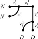
(a)

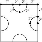
(b)

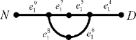
(c)

Figure 10: (a) The graph $\nicefrac{{\Gamma}}{{R_{1}}}$ with its edges labeled. (b) The graph $\Gamma$ whose relevant edges are denoted. (c) The graph $\nicefrac{{\Gamma}}{{R_{2}}}$.

Let $\lambda\in\mathbb{C}$. Let $f\in\Phi_{\nicefrac{{\Gamma}}{{R_{1}}}}(\lambda)$, $\varphi\in\Phi_{\nicefrac{{\Gamma}}{{R_{2}}}}(\lambda)$. Decoding these functions we get $\widetilde{f}_{1}\in\Phi_{\Gamma}^{R_{1}}(\lambda)$, $\widetilde{\varphi}_{1}\in\Phi_{\Gamma}^{R_{2}}(\lambda)$. Note that in the general construction we also have a superscript index denoting the number of the edge on which the function is defined. However, in this example we have a free action on the edges so that we can choose a single basis ($B$ for $\nicefrac{{\Gamma}}{{R_{1}}}$ and $\mathfrak{B}$ for $\nicefrac{{\Gamma}}{{R_{2}}}$) to work with. Using the general notation we therefore have $\forall 1\leq i\leq 6,\;\;\widetilde{f}_{1}=\widetilde{f}^{i}_{1}$ and similarly for $\widetilde{\varphi}_{1}$. Forming the inductions we have $\left\{e\widetilde{f}_{1},\,\sigma\widetilde{f}_{1}\right\}\subset\Phi_{\Gamma}^{{\rm Ind}_{H_{1}}^{D_{4}}R_{1}}(\lambda),\;\;\left\{e\widetilde{\varphi}_{1},\,\sigma\widetilde{\varphi}_{1}\right\}\subset\Phi_{\Gamma}^{{\rm Ind}_{H_{2}}^{D_{4}}R_{2}}(\lambda)$. These functions correspond to the bases $\left\{eb,\,\sigma b\right\},\,\left\{e\mathfrak{b},\,\sigma\mathfrak{b}\right\}$ and transform accordingly. We now describe the transplantation by expressing $f$ in terms of $\varphi$ (the edges’ labeling is given in figure 10).

$$f\Big{|}_{e_{1}^{1}} = \widetilde{f}_{1}\Big{|}_{\tilde{e}^{1}}=e\widetilde{f}_{1}\Big{|}_{\tilde{e}^{1}}=\nicefrac{{1}}{{\sqrt{2}}}\left(e\widetilde{\varphi}_{1}\Big{|}_{\tilde{e}^{1}}-\sigma\widetilde{\varphi}_{1}\Big{|}_{\tilde{e}^{1}}\right)$$

$$= \left(\widetilde{\varphi}_{1}\Big{|}_{\tilde{e}^{1}}-\widetilde{\varphi}_{1}\Big{|}_{\sigma^{-1}\tilde{e}^{1}}\right)=\nicefrac{{1}}{{\sqrt{2}}}\left(\widetilde{\varphi}_{1}\Big{|}_{\left(\tau\sigma^{3}\right)^{-1}\tilde{e}^{5}}-\widetilde{\varphi}_{1}\Big{|}_{\sigma^{-2}\tilde{e}^{7}}\right)$$ /12

$$= \left(\rho_{R_{2}}\left(\tau\sigma^{3}\right)\widetilde{\varphi}_{1}\Big{|}_{\tilde{e}^{5}}-\rho_{R_{2}}\left(\sigma^{2}\right)\widetilde{\varphi}_{1}\Big{|}_{\tilde{e}^{7}}\right)=\nicefrac{{1}}{{\sqrt{2}}}\left(-\widetilde{\varphi}_{1}\Big{|}_{\tilde{e}^{5}}+\widetilde{\varphi}_{1}\Big{|}_{\tilde{e}^{7}}\right)$$ /12

$$= \left(-\varphi\Big{|}_{e_{1}^{5}}+\varphi\Big{|}_{e_{1}^{7}}\right)$$ /12

$$f_{1}\Big{|}_{e_{1}^{5}} = \widetilde{f}_{1}\Big{|}_{\tilde{e}^{5}}=e\widetilde{f}_{1}\Big{|}_{\tilde{e}^{5}}=\nicefrac{{1}}{{\sqrt{2}}}\left(e\widetilde{\varphi}_{1}\Big{|}_{\tilde{e}^{5}}-\sigma\widetilde{\varphi}_{1}\Big{|}_{\tilde{e}^{5}}\right)$$

$$= \left(\widetilde{\varphi}_{1}\Big{|}_{\tilde{e}^{5}}-\widetilde{\varphi}_{1}\Big{|}_{\sigma^{-1}\tilde{e}^{5}}\right)=\nicefrac{{1}}{{\sqrt{2}}}\left(\widetilde{\varphi}_{1}\Big{|}_{\tilde{e}^{5}}-\widetilde{\varphi}_{1}\Big{|}_{\left(\tau\sigma^{3}\right)^{-1}\tilde{e}^{7}}\right)$$ /12

$$= \left(\widetilde{\varphi}_{1}\Big{|}_{\tilde{e}^{5}}-\rho_{R_{2}}\left(\tau\sigma^{3}\right)\widetilde{\varphi}_{1}\Big{|}_{\tilde{e}^{7}}\right)=\nicefrac{{1}}{{\sqrt{2}}}\left(\widetilde{\varphi}_{1}\Big{|}_{\tilde{e}^{5}}+\widetilde{\varphi}_{1}\Big{|}_{\tilde{e}^{7}}\right)$$ /12

$$= \left(\varphi\Big{|}_{e_{1}^{5}}+\varphi\Big{|}_{e_{1}^{7}}\right).$$ /12

The transplantation on all the other edges is obtained similarly and the result is

$$f\Big{|}_{e_{1}^{2}} = \left(-\varphi\Big{|}_{e_{1}^{6}}+\varphi\Big{|}_{e_{1}^{8}}\right)$$ /12

$$f\Big{|}_{e_{1}^{3}} = \left(-\varphi\Big{|}_{e_{1}^{4}}+\varphi\Big{|}_{e_{1}^{9}}\right)$$ /12

$$f\Big{|}_{e_{1}^{4}} = \left(\varphi\Big{|}_{e_{1}^{4}}+\varphi\Big{|}_{e_{1}^{9}}\right)$$ /12

$$f\Big{|}_{e_{1}^{6}} = \left(\varphi\Big{|}_{e_{1}^{6}}+\varphi\Big{|}_{e_{1}^{8}}\right).$$ /12

8 A gallery of isospectral graphs

We present three interesting examples of isospectral graphs. The first example shows that once the algebraic conditions stated in theorem 4.3 or in corollary 4.4 are satisfied, we can choose any graph that obeys the group symmetries and obtain isospectral quotients. The second example shows a symmetry group larger then $D_{4}$, as well as the effect of using different choices of representatives while constructing the quotient. The third example demonstrates the special case of a group that acts freely on a graph which enables us to get quotients whose boundary conditions are all of the Neumann type.

8.1 $G=D_{4}$ $-$ Another Choice for $\Gamma$

We present another example using the group $D_{4}$, to emphasize that it is possible to obtain isospectral quotient graphs from any graph that obeys the symmetry of $D_{4}$. We now denote the Cayley graph of $D_{4}$ with respect to the generating set $S=\{\sigma,\tau\}$ by $\Gamma$ (figure 11). Since a Cayley graph can be constructed for any discrete group, this example can easily be generalized to create other isospectral sets. The set of edges of $\Gamma$ is then $E=\{(g,gs)\}_{g\in D_{4},s\in S}$, and the action of $D_{4}$ on the edges of $\Gamma$ is by $\forall h\in D_{4}$, $h(g,gs)=(hg,hgs)$, where $s\in S$. Taking the same subgroups of $D_{4}$ and representations as in sections 3 and 5, we obtain three isospectral quotient graphs $\nicefrac{{\Gamma}}{{R_{1}}}$, $\nicefrac{{\Gamma}}{{R_{2}}}$, $\nicefrac{{\Gamma}}{{R_{3}}}$, shown in figure 12. The representatives chosen to construct the graphs are:

$$\begin{array}[]{llll}\nicefrac{{V}}{{H_{1}}}=\{e,\sigma\}&&&\nicefrac{{E}}{{H_{1}}}=\{(e,\sigma),\,(\sigma^{3},e),\,(e,\tau),\,(\sigma,\tau\sigma^{3})\}\\ \nicefrac{{V}}{{H_{2}}}=\{e,\sigma\}&&&\nicefrac{{E}}{{H_{2}}}=\{(e,\sigma),\,(\sigma^{3},e),(e,\tau),\,(\sigma,\tau\sigma^{3})\}\\ \nicefrac{{V}}{{H_{3}}}=\{e,\tau\}&&&\nicefrac{{E}}{{H_{3}}}=\{(e,\sigma),\,(\tau\sigma^{3},\tau),\,(\tau,e),(e,\tau)\}\end{array}$$

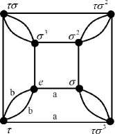
Figure 11: The Cayley graph of $D_{4}$ with the generating set $\{\sigma,\tau\}$. The lengths of some edges of this quantum graph are marked.

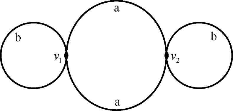
$$A_{v_{1}}=A_{v_{2}}=\left(\scriptsize{\begin{array}[]{cccc}1&1&0&0\\ 1&0&1&0\\ 1&0&0&1\\ 0&0&0&0\end{array}}\right)$$

$$B_{v_{1}}=B_{v_{2}}=\left(\scriptsize{\begin{array}[]{cccc}0&0&0&0\\ 0&0&0&0\\ 0&0&0&0\\ 1&-1&-1&-1\end{array}}\right)$$

(a)

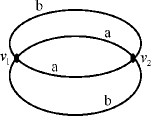
$\begin{array}[]{cc}{\scriptstyle A_{v_{1}}=\left(\scriptsize{\begin{array}[]{cccc}1&1&0&0\\ 1&0&1&0\\ 1&0&0&1\\ 0&0&0&0\end{array}}\right)}&{\scriptstyle B_{v_{1}}=\left(\scriptsize{\begin{array}[]{cccc}0&0&0&0\\ 0&0&0&0\\ 0&0&0&0\\ 1&-1&-1&-1\end{array}}\right)}\\ \\ {\scriptstyle A_{v_{2}}=\left(\scriptsize{\begin{array}[]{cccc}1&1&0&0\\ 1&0&-1&0\\ 1&0&0&1\\ 0&0&0&0\end{array}}\right)}&{\scriptstyle B_{v_{2}}=\left(\scriptsize{\begin{array}[]{cccc}0&0&0&0\\ 0&0&0&0\\ 0&0&0&0\\ -1&1&-1&1\end{array}}\right)}\end{array}$

(b)

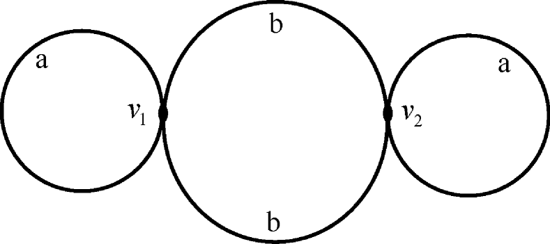
$$A_{v_{1}}=A_{v_{2}}=\left(\scriptsize{\begin{array}[]{cccc}i&1&0&0\\ i&0&1&0\\ i&0&0&1\\ 0&0&0&0\end{array}}\right)$$

$$B_{v_{1}}=B_{v_{2}}=\left(\scriptsize{\begin{array}[]{cccc}0&0&0&0\\ 0&0&0&0\\ 0&0&0&0\\ -i&1&1&1\end{array}}\right)$$

(c)

Figure 12: The three quotient graphs obtained from the Cayley graph. (a) $\nicefrac{{\Gamma}}{{R_{1}}}$, (b)$\nicefrac{{\Gamma}}{{R_{2}}}$, (c) $\nicefrac{{\Gamma}}{{R_{3}}}$. The matrices describe the boundary conditions at the various vertices. The diagrams on the left relate the edges to the rows of the corresponding matrices, numbered 1-4.

8.2 $G=O_{h}$ $-$ Freedom to Choose Representatives

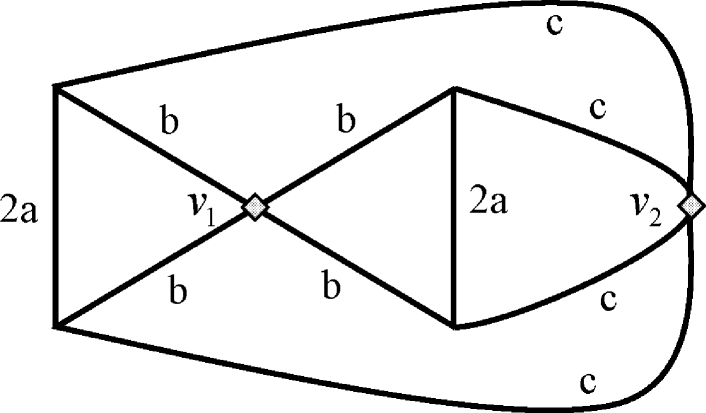
$\begin{array}[]{cc}{\scriptstyle A_{v_{1}}=\left(\scriptsize{\begin{array}[]{cccc}1&c&0&-s\\ 0&s&-1&c\\ 0&0&0&0\\ 0&0&0&0\end{array}}\right)}&{\scriptstyle B_{v_{1}}=\left(\scriptsize{\begin{array}[]{cccc}0&0&0&0\\ 0&0&0&0\\ 1&-c&0&s\\ 0&-s&-1&-c\end{array}}\right)}\\ \\ {\scriptstyle A_{v_{2}}=\left(\scriptsize{\begin{array}[]{cccc}1&c&0&s\\ 0&s&1&-c\\ 0&0&0&0\\ 0&0&0&0\end{array}}\right)}&{\scriptstyle B_{v_{2}}=\left(\scriptsize{\begin{array}[]{cccc}0&0&0&0\\ 0&0&0&0\\ 1&-c&0&-s\\ 0&-s&1&c\end{array}}\right)}\end{array}$

where $c=cos(\pi/3)$ and $s=sin(\pi/3)$

(a)

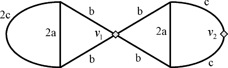
$\begin{array}[]{cc}{\scriptstyle A_{v_{1}}=\left(\scriptsize{\begin{array}[]{cccc}1&c&0&-s\\ 0&s&-1&c\\ 0&0&0&0\\ 0&0&0&0\end{array}}\right)}&{\scriptstyle B_{v_{1}}=\left(\scriptsize{\begin{array}[]{cccc}0&0&0&0\\ 0&0&0&0\\ 1&-c&0&s\\ 0&-s&-1&-c\end{array}}\right)}\\ \\ {\scriptstyle A_{v_{2}}=}\left(\scriptsize{\begin{array}[]{cccc}1&1\\ 0&0\end{array}}\right)&{\scriptstyle B_{v_{2}}=}\left(\scriptsize{\begin{array}[]{cccc}0&0\\ 1&-1\end{array}}\right)\end{array}$

(b)

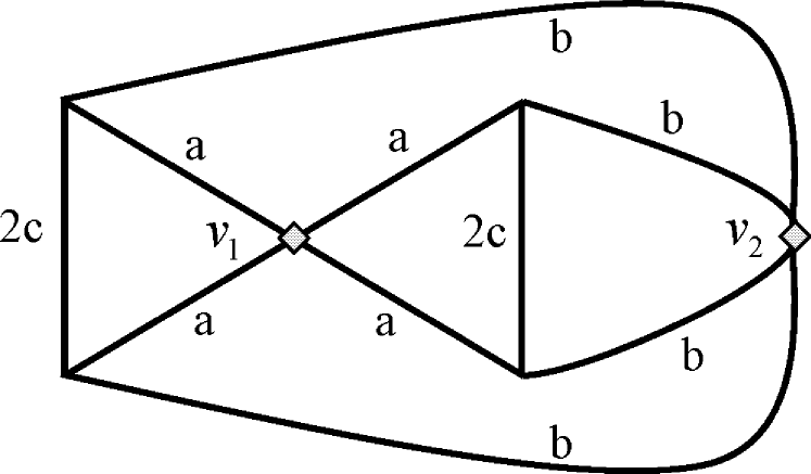
$\begin{array}[]{cc}{\scriptstyle A_{v_{1}}=\left(\scriptsize{\begin{array}[]{cccc}1&c&0&s\\ 0&s&1&-c\\ 0&0&0&0\\ 0&0&0&0\end{array}}\right)}&{\scriptstyle B_{v_{1}}=\left(\scriptsize{\begin{array}[]{cccc}0&0&0&0\\ 0&0&0&0\\ 1&-c&0&-s\\ 0&-s&1&c\end{array}}\right)}\\ \\ {\scriptstyle A_{v_{2}}=\left(\scriptsize{\begin{array}[]{cccc}1&c&0&-s\\ 0&s&1&c\\ 0&0&0&0\\ 0&0&0&0\end{array}}\right)}&{\scriptstyle B_{v_{2}}=\left(\scriptsize{\begin{array}[]{cccc}0&0&0&0\\ 0&0&0&0\\ 1&-c&0&s\\ 0&-s&1&-c\end{array}}\right)}\end{array}$

(c)

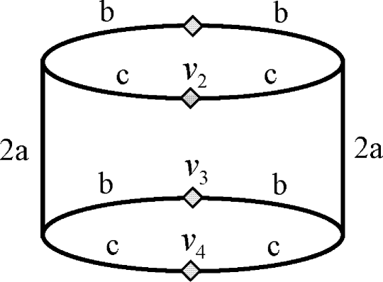
$\begin{array}[]{cc}{\scriptstyle A_{v_{1}}=A_{v_{3}}=\left(\scriptsize{\begin{array}[]{cc}1+c&-s\\ 0&0\end{array}}\right)}&{\scriptstyle A_{v_{2}}=\left(\scriptsize{\begin{array}[]{cc}1+c&s\\ 0&0\end{array}}\right)}\\ \\ {\scriptstyle B_{v_{1}}=B_{v_{3}}=\left(\scriptsize{\begin{array}[]{cc}0&0\\ 1-c&s\end{array}}\right)}&{\scriptstyle B_{v_{2}}=\left(\scriptsize{\begin{array}[]{cc}0&0\\ 1-c&-s\end{array}}\right)}\end{array}$

(d)

Figure 13: The isospectral graphs obtained from the cube. (a)-(c) are all $\nicefrac{{\Gamma}}{{R_{1}}}$, formed by choosing different representatives for $\nicefrac{{E}}{{O}}$ and (d) is the graph $\nicefrac{{\Gamma}}{{R_{2}}}$. Unless stated otherwise, Neumann boundary conditions are assumed. The boundary conditions of the marked vertices are given by the matrices on the right.

We now consider a larger group, and treat $O_{h}$, the group of symmetries of the cube. The group $O_{h}$ contains forty-eight elements: the identity, twenty-three rotations, and twenty-four reflections. A fundamental domain for the action of $O_{h}$ on the cube is a tetrahedron. Each of the forty-eight tetrahedra that together form the cube has one of its faces along the external boundary of the cube, and its other three faces inside the cube. We begin by describing a graph, denoted by $\Gamma$, that obeys the symmetries of $O_{h}$. We consider star graphs with three edges, such that each tetrahedron contains one such star graph, and the edges of the star graph are connected to the centre of the interior faces of the tetrahedron (one edge goes to each face). This star graph is constructed to have three edges of different lengths, labeled $a,b$, and $c$. Any two star graphs in neighbouring tetrahedra are then connected at the center of their common face. $\Gamma$ is the union of these star graphs. It is a three-regular, bipartite graph, with forty-eight vertices, and seventy-two edges of lengths $2a,2b$ and $2c$, each with equal multiplicity. We will use the subgroups $O,T_{d}\leq O_{h}$, along with appropriate representations, to form the isospectral quotient graphs.

We first consider the subgroup $O\leq O_{h}$, known as the octahedral group, which contains the identity and the twenty-three rotation elements. We take representatives for $\nicefrac{{E}}{{O}}$ and $\nicefrac{{V}}{{O}}$. Since $O$ is a subgroup of index two, one possiblitiy is to choose the edges and vertices contained in two tetrahedra as representatives. $O$ has two 1-dimensional, one 2-dimensional, and two 3-dimensional irreducible representations [36]. We work with the two dimensional representation, using the basis given in [36] and we denote it as $R_{1}$. The quotient graph $\nicefrac{{\Gamma}}{{R_{1}}}$ is shown in figure 13(a). As noted in sections 6, 7.4, it is possible to make different choices for the representatives. We present three different quotient graphs for $\nicefrac{{\Gamma}}{{R_{1}}}$, corresponding to three different choices of representatives, in figure 13(a)-(c).

We now examine the subgroup $T_{d}\leq O_{h}$. The vertices of the cube consist of two sets, each of which forms the vertices of an equilateral tetrahedron. $T_{d}$ contains all the elements of $O_{h}$ whose action does not mix between the two sets. It should be noted that $O\cong T_{d}\cong S_{4}$. In particular, $T_{d}$ and $O$ have the same irreducible representations. We will take the matrix representation that was used for $O$, and use it for $T_{d}$, denoting it by $R_{2}$. The quotient graph $\nicefrac{{\Gamma}}{{R_{2}}}$ is shown in figure 13(d).
The isospectrality of the quotient graphs formed from $O$ and $T_{d}$ follows from the fact that ${\rm Ind}_{O}^{O_{h}}R_{1}\cong{\rm Ind}_{T_{d}}^{O_{h}}R_{2}$.

8.3 $G=D_{3}$ $-$ A free action on $\Gamma$

We now consider an example that demonstrates the possibility of constructing quotient graphs that have only Neumann boundary conditions. We show that this can be achieved even when dividing by multidimensional representations. We consider the graph $\Gamma$, shown in figure 14, which is symmetric under the action of $D_{3}\cong S_{3}$. The group acts freely on both the vertices and edges of $\Gamma$. This is ensured by having the circles perpendicular to the plane of the triangle. We have $D_{3}=\{e,\sigma,\sigma^{2},\tau,\tau\sigma,\tau\sigma^{2}\}$, where $\sigma$ is a rotation of $\nicefrac{{2\pi}}{{3}}$ about the axis perpendicular to the plane of the triangle, and $\tau$ is a rotation of $\pi$ about the height of the triangle.

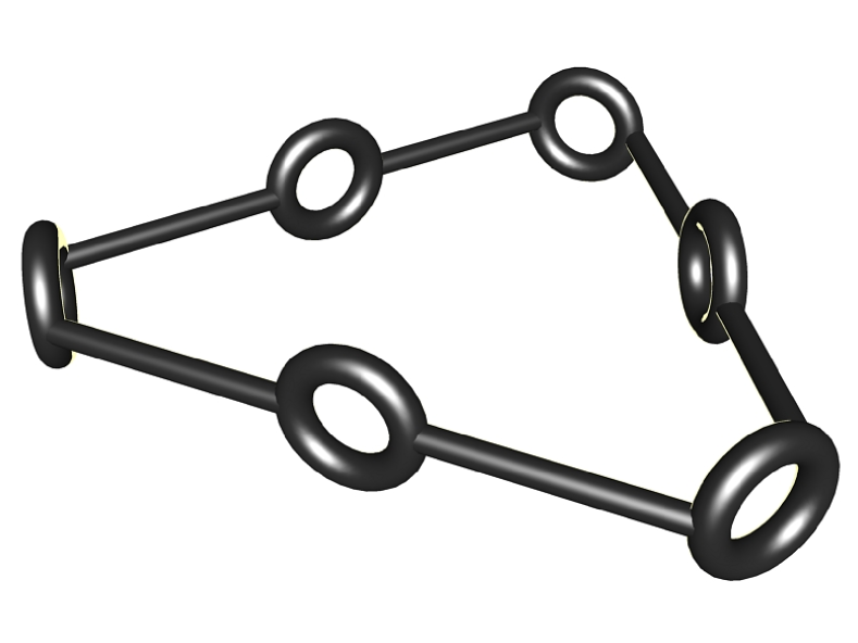
(a)

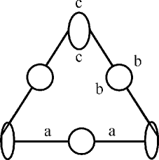
(b)

Figure 14: Two visualizations of the graph $\Gamma$ which is symmetric under $D_{3}$. (a) A three dimensional visualization. The loops are perpendicular to the plane of the triangle. $\sigma$ is a rotation of $\nicefrac{{2\pi}}{{3}}$ about an axis perpendicular to the plane of the triangle, and $\tau$ is a rotation of $\pi$ about a height of the triangle. (b) A two dimensional visualization whose edges’ lengths are marked.

Rather than working with representations of various subgroups, we use various bases of a representation of the entire group to create the quotient graphs. $D_{3}$ has three irreducible representations: the trivial representation $S_{1}$, the sign representation $S_{2}$, and the standard representation $S_{3}$, which is of dimension two. We take the eight-dimensional representation $R~{}=~{}3S_{1}+S_{2}+2S_{3}$. We begin by choosing a basis such that the matrix representation of $R$ is block diagonalized as follows:

$$\left(\begin{array}[]{c|c|c}S_{1}+S_{2}+2S_{3}&\lx@intercol\hfil\hfil\lx@intercol\\ \cline{1-2}\cr&S_{1}\\ \cline{2-3}\cr\lx@intercol\hfil\hfil\lx@intercol\vrule\lx@intercol&S_{1}\end{array}\right).$$

This choice of basis is not unique. We therefore specify it, by identifying the top block as the regular representation of $D_{3}$, and taking the standard basis for this representation. Due to the fact that the matrix representation is block diagonalized, the quotient graph created consists of three disjoint graphs. Each graph corresponds to one block, and these are shown in figure 15.

(a)

(b)

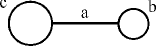
(c)

Figure 15: The first quotient graph $\nicefrac{{\Gamma}}{{S_{1}+S_{2}+2S_{3}}}\cup\nicefrac{{\Gamma}}{{S_{1}}}\cup\nicefrac{{\Gamma}}{{S_{1}}}$. All vertices have Neumann boundary conditions. (a) The graph formed from the first block of the representation. Note that in this case, we have recovered the original graph. (b)-(c) Two copies, coming from the two blocks containing the trivial representation.

Note that this representation consists of permutation matrices. This, together with the fact that the action of $D_{3}$ on $\Gamma$ is free, ensures Neumann boundary conditions on the quotient graph. We now choose a new basis, such that the matrix representation of $R$ takes the form:

$$\left(\begin{array}[]{c|c|c}S_{1}+S_{3}&\lx@intercol\hfil\hfil\lx@intercol\\ \cline{1-2}\cr&S_{1}+S_{3}\\ \cline{2-3}\cr\lx@intercol\hfil\hfil\lx@intercol\vrule\lx@intercol&S_{1}+S_{2}\end{array}\right).$$

Again we must further specify the choice of basis. Each of the first two blocks is the permutation representation of the symmetric group of size three, and we choose its standard basis. For the third block, we choose the basis in which:

$$\sigma\mapsto\left(\begin{array}[]{cc}1&0\\ 0&1\end{array}\right),\;\;\tau\mapsto\left(\begin{array}[]{cc}0&1\\ 1&0\end{array}\right)\,.$$

Using this basis, we again obtain a quotient graph consisting of three disjoint graphs, corresponding to the three blocks of the matrix representation, as shown in figure 16. This quotient also has only Neumann boundary conditions for the same reason. The two quotient graphs, namely $\nicefrac{{\Gamma}}{{S_{1}+S_{2}+2S_{3}}}\cup\nicefrac{{\Gamma}}{{S_{1}}}\cup\nicefrac{{\Gamma}}{{S_{1}}}$ and $\nicefrac{{\Gamma}}{{S_{1}+S_{3}}}\cup\nicefrac{{\Gamma}}{{S_{1}+S_{3}}}\cup\nicefrac{{\Gamma}}{{S_{1}+S_{2}}}$, are isospectral.

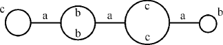
(a)

(b)

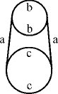
(c)

Figure 16: The second quotient graph $\nicefrac{{\Gamma}}{{S_{1}+S_{3}}}\cup\nicefrac{{\Gamma}}{{S_{1}+S_{3}}}\cup\nicefrac{{\Gamma}}{{S_{1}+S_{2}}}$. All vertices have Neumann boundary conditions. (a)-(b) The graphs formed from the first two blocks of the representation. (c) The graph obtained from the third block.

Remark.

As a matter of fact, all the quotients obtained in this subsection can also be obtained as quotients by the trivial representations of $D_{3}$’s subgroups, as

$${\rm Ind}_{D_{3}}^{D_{3}}\mathbf{1} \cong S_{1}$$

$${\rm Ind}^{D_{3}}_{\left<\sigma\right>}\mathbf{1} \cong S_{1}+S_{2}$$

$${\rm Ind}^{D_{3}}_{\left<\tau\right>}\mathbf{1} \cong S_{1}+S_{3}$$

$${\rm Ind}^{D_{3}}_{\left\{id\right\}}\mathbf{1} \cong S_{1}+S_{2}+2S_{3}.$$

9 Drums and Manifolds

We now apply theorem (4.3) to other objects. In particular, we reconstruct some existing examples using our method, and comment on some new results.

9.1 Jakobson, Levitin, et al.

We begin by examining the isospectral domains presented by Jakobson et al. and Levitin et al. [9, 10]. It is possible to recover all the isospectral examples described in these papers as quotients by representations with isomorphic inductions. We consider first an interesting example, consisting of the four isospectral domains shown in figure 17 (See also figure 7 in [10]).

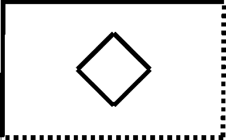
$\nicefrac{{\mathbb{T}}}{{R_{1}\otimes R_{1}}}$

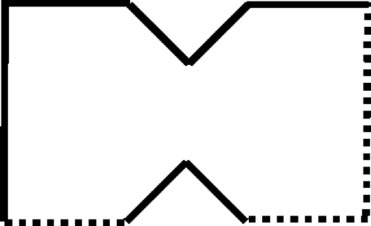
$\nicefrac{{\mathbb{T}}}{{R_{1}\otimes R_{2}}}$

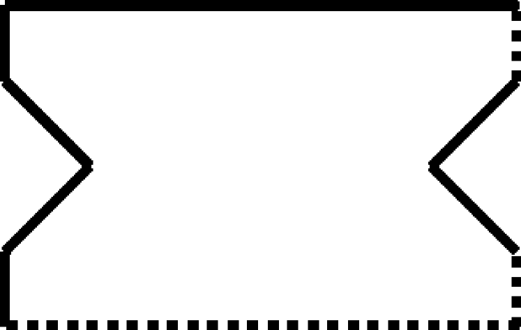
$\nicefrac{{\mathbb{T}}}{{R_{2}\otimes R_{1}}}$

$\nicefrac{{\mathbb{T}}}{{R_{2}\otimes R_{2}}}$

Figure 17: The four isospectral domains presented in [10], obtained as quotients of the torus $\mathbb{T}$ (figure 18). solid lines indicate Dirichlet boundary conditions, and dotted ones Neumann.

We take a torus, $\mathbb{T}$, with sixteen diamond-shaped holes, as shown in figure 18. We can express the torus as $T_{a}\times T_{b}$, where $T_{a},\,T_{b}$ are circles with circumferences $a$ and $b$ respectively. Taking a rigid action of $D_{4}$ on each of the circles $T_{a}$ and $T_{b}$, we obtain an action of $G=D_{4}\times D_{4}$ on the torus $T_{a}\times T_{b}$: the action of the first $D_{4}$ in the direct product is by horizontal translations and reflections, and that of the second $D_{4}$ is by vertical ones. For example, the element $(\sigma,e)$ transforms $\mathbb{T}$ rigidly onto itself so that the four columns of diamonds are cyclically shifted by one, and the element $(\tau,e)$ swaps the first column with the fourth, and the second with the third. Similarly, the action of elements of the form $(e,g)$ is by transformations that permute the rows of diamonds.

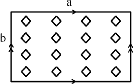
Figure 18: The torus $\mathbb{T}$, of which the four domains in figure 17 are quotients.

Adopting the notations of section 3, we examine the subgroups $\left\{H_{i}\times H_{j}\right\}_{i,j\in\left\{1,2\right\}}$ of $D_{4}\times D_{4}$ and their corresponding representations $\left\{R_{i}\otimes R_{j}\right\}_{i,j\in\left\{1,2\right\}}$. Since ${\rm Ind}_{H_{1}}^{D_{4}}R_{1}\cong{\rm Ind}_{H_{2}}^{D_{4}}R_{2}$, all of these representations have isomorphic inductions in $D_{4}\times D_{4}$. Applying corollary 4.4, we obtain that $\left\{\nicefrac{{\mathbb{T}}}{{R_{i}\otimes R_{j}}}\right\}_{i,j\in\left\{1,2\right\}}$ are isospectral (figure 17).

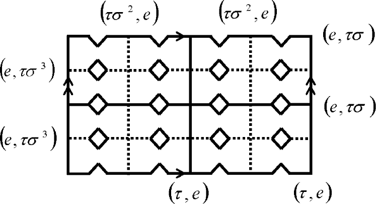
(a)

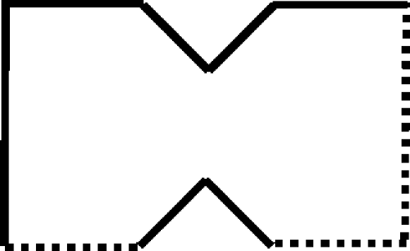
(b)

Figure 19: (a) The information we have on $\tilde{f}\in\Phi_{\mathbb{T}}^{R_{1}\otimes R_{2}}(\lambda)$. The function vanishes along the solid lines and its normal derivatives at the dotted lines are zero. (b) The quotient planar domain $\nicefrac{{\mathbb{T}}}{{{R_{1}\otimes R_{2}}}}$ which encodes this information. Solid lines stand for Dirichlet boundary conditions and dotted lines for Neumann.

To demonstrate how the technicalities work for these domains, we construct $\nicefrac{{\mathbb{T}}}{{R_{1}\otimes R_{2}}}$. From (3.2) and (3.4), we obtain information on $\tilde{f}\in\Phi_{\mathbb{T}}^{R_{1}\otimes R_{2}}(\lambda)$: we see that $\tilde{f}$ vanishes on the axes of reflection of $(\tau,e)$, as it is anti-symmetric with respect to this reflection, and similarly for $(e,\tau\sigma)$. Since $\tilde{f}$ is symmetric with respect to the axes of $(\tau\sigma^{2},e)$ and $(e,\tau\sigma^{3})$, its normal derivatives with respect to these axes are zero. This is summarized in figure 19(a) and the resulting quotient is shown in figure 19(b). Notice that the two parts of figure 19 serve the same purpose as those of figure 3, i.e., to demonstrate how the information on a function belonging to a certain isotypic component is encoded in the boundary conditions of the quotient. We end by remarking that all the constructions demonstrated in section 5 can be applied analogously to $\mathbb{T}$ to enlarge the isospectral quartet in figure 17. However, the quotients obtained from most choices of representations and bases will not be planar domains, or even manifolds. For example, consider the representation $R_{3}$ of $H_{3}$, given in (5.2). The quotient $\nicefrac{{\mathbb{T}}}{{R_{1}\otimes R_{3}}}$ (figure 20) is a cylinder with Dirichlet and Neumann conditions at its boundaries, and a “factor of $i$” condition along a section line normal to the boundaries (compare with the quotient $\nicefrac{{\Gamma}}{{R_{3}}}$ introduced in section 5). This quotient is a manifold with a singularity. Other types of singularities may arise when considering quotients with respect to multidimensional representations.

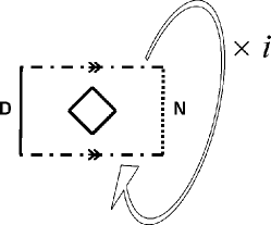
Figure 20: The quotient $\nicefrac{{\mathbb{T}}}{{{R_{1}\otimes R_{3}}}}$. Solid lines stand for Dirichlet boundary conditions and dotted lines for Neumann. There is a factor of i between the values and derivatives at the top and bottom edges.

We now examine a more general example presented in [10]. Consider the cylindrical drum $\mathbb{D}$, shown in figure 21. In the figure, the left and the right edges are identified. The three dots imply that the basic pattern which appears in figure 22 is repeated and $\mathbb{D}$ consists of $8n$ copies of it. $\mathbb{D}$ is symmetric under the action of the dihedral group $D_{4n}$, where $\sigma$ rotates the cylinder and $\tau$ is a reflection whose axis is shown in figure 21.

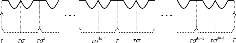
Figure 21: The cylindrical drum $\mathbb{D}$. The left and right edges are identified. Solid lines stand for Dirichlet boundary conditions and dotted ones for Neumann. The reflection elements in $D_{4n}$ and their axes are indicated.

Figure 22: A fundamental domain of $\mathbb{D}$ under the action of $D_{4n}$.

We consider the subgroups $H_{1},H_{2}\leq D_{4n}$, where

$$H_{1} = \{e,\,\tau,\,\tau\sigma^{2n},\,\sigma^{2n}\}$$

$$H_{2} = \{e,\,\tau\sigma,\,\tau\sigma^{2n+1},\,\sigma^{2n}\},$$

equipped with the one-dimensional representations

$$R_{1} : \left\{\begin{array}[]{llll}e\mapsto\left(1\right),&\tau\mapsto\left(-1\right),&\tau\sigma^{2n}\mapsto\left(1\right),&\sigma^{2n}\mapsto\left(-1\right)\end{array}\right\}$$

$$R_{2} : \left\{\begin{array}[]{llll}e\mapsto\left(1\right),&\tau\sigma\mapsto\left(1\right),&\tau\sigma^{2n+1}\mapsto\left(-1\right),&\sigma^{2n}\mapsto\left(-1\right)\end{array}\right\}.$$

We find that ${\rm Ind}_{H_{1}}^{D_{4n}}R_{1}\cong{\rm Ind}_{H_{2}}^{D_{4n}}R_{2}$, and therefore we can form two isospectral quotients, each one a quarter the width of the original drum, with Dirichlet boundary conditions on one side, and Neumann on the other. In figure 23 the drum $\mathbb{D}$ and the resulting quotients are shown for the case $n=2$. In conclusion, we have provided an alternate proof for theorem 4.2 in [10]. In fact, this proof is valid for any number $n$, whereas the original theorem in [10] treated only the case $n=2^{k}$. The reader might wonder why did we limit our attention to $D_{4n}$. The answer is that if we consider the more general $D_{n}$, then in order to define $H_{1}$ and $H_{2}$, $n$ must be even. If $n$ is even, but not a multiple of four, then the proof works, but in that case $H_{1}$ and $H_{2}$ are also conjugate in $D_{4}$, so that the isospectral domains thus obtained are also isometric.

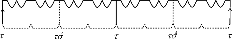
(a)

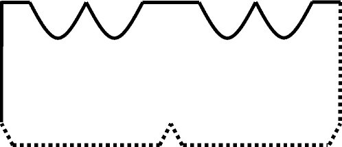
(b) - $\nicefrac{{\mathbb{D}}}{{R_{1}}}$

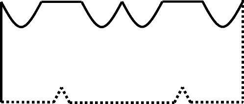
(c) - $\nicefrac{{\mathbb{D}}}{{R_{2}}}$

Figure 23: (a) The information we have on $\tilde{f}\in\Phi_{\mathbb{D}}^{R_{1}}(\lambda)$. The function vanishes along the solid lines, and its normal derivatives at the dotted lines are zero. (b),(c) The quotient planar domains $\nicefrac{{\mathbb{D}}}{{R_{1}}}$ and $\nicefrac{{\mathbb{D}}}{{R_{2}}}$. Solid lines stand for Dirichlet boundary conditions and dotted ones for Neumann. These domains illustrate the case $n=2$.

9.2 Gordon, Webb and Wolpert

The famous domains of Gordon, Webb and Wolpert, originally presented in [6, 7], can be similarly constructed by our method. Buser et al. [8] have shown that they can be constructed as quotients of the hyperbolic plane. This is done by considering an epimorphism from the symmetry group of this plane onto $\mathrm{PSL_{3}\left(\mathbb{F}_{2}\right)}$, and taking the inverse images of two subgroups in $\mathrm{PSL_{3}\left(\mathbb{F}_{2}\right)}$, each isomorphic to $S_{4}$. In our formalism, the drums of Gordon et al. are obtained (with Neumann boundary conditions) from the quotient of the hyperbolic plane by the corresponding trivial representations of $S_{4}$. Using the sign representation of $S_{4}$ instead we obtain the same drums with different boundary conditions (figure 24). The conditions of corollary 4.4 are satisfied in this case as well, so that this pair of drums is isospectral. A more detailed explanation is given in [27].

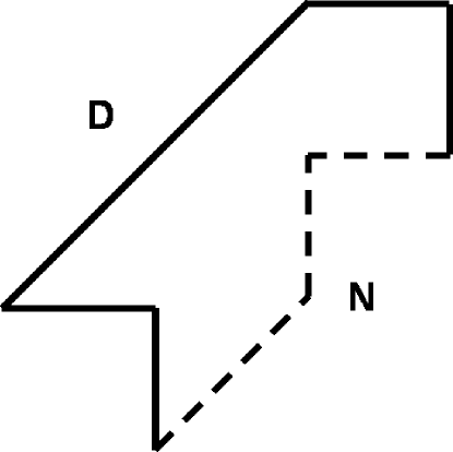
(a)

(b)

Figure 24: The isospectral drums of Gordon et al. with new boundary conditions.

9.3 Chapman’s two piece band

In $D_{4}$ there are no Sunada pairs, i.e., there are no nonconjugate subgroups $A,B~{}\leq~{}D_{4}$ whose trivial representations satisfy $\mathrm{Ind}_{A}^{D_{4}}\mathbf{1}_{A}\cong\mathrm{Ind}_{B}^{D_{4}}\mathbf{1}_{B}$. However, by simple arithmetic we can extract isospectrality even from these “basic ingredients”.

We note that if $\left\{R_{i}\right\}_{i=1}^{n}$ are representations of $G$, then the disjoint union $\bigcup\limits_{i=1}^{n}\nicefrac{{\Gamma}}{{R_{i}}}$ is isospectral to $\nicefrac{{\Gamma}}{{\bigoplus\limits_{i=1}^{n}\!\!R_{i}}}$, as we have $\Phi_{\bigcup\limits_{i=1}^{n}\nicefrac{{\Gamma}}{{R_{i}}}}\left(\lambda\right)=\bigoplus\limits_{i=1}^{n}\Phi_{\nicefrac{{\Gamma}}{{R_{i}}}}\left(\lambda\right)$, so that

$$\sigma_{\bigcup\limits_{i=1}^{n}\nicefrac{{\Gamma}}{{R_{i}}}}\left(\lambda\right)=\sum\limits_{i=1}^{n}\left\langle\chi_{R_{i}},\chi_{\Phi_{\Gamma}\left(\lambda\right)}\right\rangle_{G}=\left\langle\chi_{\bigoplus\limits_{i=1}^{n}\!\!R_{i}},\chi_{\Phi_{\Gamma}\left(\lambda\right)}\right\rangle_{G}=\sigma_{\nicefrac{{\Gamma}}{{\bigoplus\limits_{i=1}^{n}\!\!R_{i}}}}\left(\lambda\right)$$

(this was implicitly manifested in section 8.3). Combining this with theorem 4.3, we obtain the following: if $\left\{H_{i}\right\}$,$\left\{H^{\prime}_{j}\right\}$ are finite sets of subgroups of $G$, with corresponding representations $\left\{R_{i}\right\}$, $\left\{R_{j}^{\prime}\right\}$, such that $\bigoplus_{i}\mathrm{Ind}_{H_{i}}^{G}R_{i}\cong\bigoplus_{j}\mathrm{Ind}_{H^{\prime}_{j}}^{G}R^{\prime}_{j}$, then $\bigcup_{i}\nicefrac{{\Gamma}}{{R_{i}}}$ is isospectral to $\bigcup_{j}\nicefrac{{\Gamma}}{{R^{\prime}_{j}}}$.

We recall the subgroups $H_{1},H_{2},H_{3}\leq D_{4}$ from sections 3, 5 and consider also $H_{4}=\left\{e,\tau\sigma^{2}\right\}$ and $H_{5}=\left\{e,\tau\sigma\right\}$. Even though no two inductions among $\left\{\mathrm{Ind}_{H_{i}}^{D_{4}}\mathbf{1}_{H_{i}}\right\}_{i=1}^{5}$ are isomorphic, we do have that $\mathrm{Ind}_{H_{1}}^{D_{4}}\mathbf{1}_{H_{1}}\oplus\mathrm{Ind}_{H_{5}}^{D_{4}}\mathbf{1}_{H_{5}}\cong\mathrm{Ind}_{H_{2}}^{D_{4}}\mathbf{1}_{H_{2}}\oplus\mathrm{Ind}_{H_{4}}^{D_{4}}\mathbf{1}_{H_{4}}$. By the observation above, if $D_{4}$ acts on some object $\Gamma$, then $\nicefrac{{\Gamma}}{{\mathbf{1}_{H_{1}}}}\cup\nicefrac{{\Gamma}}{{\mathbf{1}_{H_{5}}}}$ is isospectral to $\nicefrac{{\Gamma}}{{\mathbf{1}_{H_{2}}}}\cup\nicefrac{{\Gamma}}{{\mathbf{1}_{H_{4}}}}$.

(a)

(b)

Figure 25: (a) A square $\mathbb{S}$, on which $D_{4}$ acts, with the axes of reflection elements marked. (b) Fundamental domains for the actions of $H_{1}=\left\langle\tau,\tau\sigma^{2}\right\rangle$, $H_{2}=\left\langle\tau\sigma,\tau\sigma^{3}\right\rangle$, $H_{4}=\left\langle\tau\sigma^{2}\right\rangle$, $H_{5}=\left\langle\tau\sigma\right\rangle$ on $\mathbb{S}$.

In figure 25, part (a) displays a square $\mathbb{S}$, of side length 2, on which $D_{4}$ acts, and part (b) displays fundamental domains for the actions of $D_{4}$’s subgroups $\left\{H_{i}\right\}_{i=1,2,4,5}$. If we supply $\mathbb{S}$ with Neumann boundary conditions, we obtain that $\left\{\nicefrac{{\mathbb{S}}}{{\mathbf{1}_{H_{i}}}}\right\}$ are the domains shown in figure 25(b), also with Neumann boundary conditions. The isospectrality of $\nicefrac{{\mathbb{S}}}{{\mathbf{1}_{H_{1}}}}\cup\nicefrac{{\mathbb{S}}}{{\mathbf{1}_{H_{5}}}}$ and $\nicefrac{{\mathbb{S}}}{{\mathbf{1}_{H_{2}}}}\cup\nicefrac{{\mathbb{S}}}{{\mathbf{1}_{H_{4}}}}$ is a known example constructed by Chapman [29], which shows that “one cannot hear the shape of a two-piece band” [35]. Chapman obtains this isospectral example by manipulating the drums of Gordon et al. $-$ he enlarges the number of connected components by cutting the basic building block, and then cancels out identical components in the two shapes. Chapman shows that these domains are also isospectral if the Neumann conditions at the boundaries are replaced by Dirichlet ones, and we would like to establish this as well. A reasonable guess would be to try $\mathbb{D}$, a square identical to $\mathbb{S}$ but with Dirichlet boundary conditions. This, however, leads to isospectrality of domains with mixed boundary conditions (figure 26).

Figure 26: Various quotients of $\mathbb{D}$, the square in figure 25(a) with Dirichlet boundary (Solid lines stand for Dirichlet boundary conditions and dashed ones for Neumann). $\nicefrac{{\mathbb{D}}}{{\mathbf{1}_{H_{1}}}}\cup\nicefrac{{\mathbb{D}}}{{\mathbf{1}_{H_{5}}}}$ is isospectral to $\nicefrac{{\mathbb{D}}}{{\mathbf{1}_{H_{2}}}}\cup\nicefrac{{\mathbb{D}}}{{\mathbf{1}_{H_{4}}}}$.

In figure 26, the Dirichlet edges are the remnants of $\mathbb{D}$’s boundary, whereas the Neumann edges are the traces of the reflections by which the quotients were taken. One is thus led to consider the following representations:

$$R^{\prime}_{1} : \left\{\begin{array}[]{llll}e\mapsto\left(1\right),&\tau\mapsto\left(-1\right),&\tau\sigma^{2}\mapsto\left(-1\right),&\sigma^{2}\mapsto\left(1\right)\end{array}\right\}$$

$$R^{\prime}_{2} : \left\{\begin{array}[]{llll}e\mapsto\left(1\right),&\tau\sigma\mapsto\left(-1\right),&\tau\sigma^{3}\mapsto\left(-1\right),&\sigma^{2}\mapsto\left(1\right)\end{array}\right\}$$

$$R^{\prime}_{4} : \left\{\begin{array}[]{ll}e\mapsto\left(1\right),&\tau\sigma^{2}\mapsto\left(-1\right)\end{array}\right\}$$

$$R^{\prime}_{5} : \left\{\begin{array}[]{ll}e\mapsto\left(1\right),&\tau\sigma\mapsto\left(-1\right)\end{array}\right\}\>.$$

In $\left\{R^{\prime}_{i}\right\}$, the reflection elements are sent to $\left(-1\right)$, so that the corresponding quotients encode functions which are antisymmetric at the corresponding axes, hence vanishing along them. The quotients $\left\{\nicefrac{{\mathbb{D}}}{{R^{\prime}_{i}}}\right\}_{i=1,2,4,5}$ are indeed the domains presented in figure 25(b) with Dirichlet boundary conditions, and upon verifying that $\mathrm{Ind}_{H_{1}}^{D_{4}}R^{\prime}_{1}\oplus\mathrm{Ind}_{H_{5}}^{D_{4}}R^{\prime}_{5}\cong\mathrm{Ind}_{H_{2}}^{D_{4}}R^{\prime}_{2}\oplus\mathrm{Ind}_{H_{4}}^{D_{4}}R^{\prime}_{4}$, we obtain the isospectrality we have sought. Note that by taking $\left\{\nicefrac{{\mathbb{S}}}{{R^{\prime}_{i}}}\right\}_{i=1,2,4,5}$, we would have again obtained the mixed isospectral example in figure 26, but with the Dirichlet and Neumann conditions swapped. We end by remarking that as usual, one can extend the isospectral families above by considering other bases for the representations $\mathrm{Ind}_{H_{1}}^{D_{4}}\mathbf{1}_{H_{1}}\oplus\mathrm{Ind}_{H_{5}}^{D_{4}}\mathbf{1}_{H_{5}}$ and $\mathrm{Ind}_{H_{1}}^{D_{4}}R^{\prime}_{1}\oplus\mathrm{Ind}_{H_{5}}^{D_{4}}R^{\prime}_{5}$, but that in the general case the objects thus obtained will no longer be planar domains.

10 Summary and open questions

This paper describes a method which enables one to construct isospectral objects, such as quantum graphs and drums. The algebraic component of the underlying theory suggests theorem 4.3 and corollary 4.4 as our main tools for producing isospectral objects. Their assumptions are less strict than those of Sunada’s theorem [2] and this allows more degrees of freedom in the isospectral search. Another ingredient is the assembly process of the so called quotient graphs, whose construction accounts for yet more liberty. We found that for a graph $\Gamma$ with a symmetry group $G$ and a representation $R$ of the group, we have a variety of choices to make for the fundamental domain of the action of $G$ on $\Gamma$ and also for the basis with respect to which $R$ is presented. These different possibilities yield (possibly) different quotient graphs $\nicefrac{{\Gamma}}{{R}}$, all isospecral to each other. We wish to offer two perspectives on this dizzying freedom. On the one hand, it invites us to test the strength of the method. Namely, given two isospectral objects, can it be decided whether they arise as quotients of some common object? We touched this question so far merely by reconstructing some known isospectral objects in terms of our method. On the other hand, it prompts one to classify these sources of isospectrality and understand the interrelationships between them. A fundamental question in this context is whether for $R$ as above, there exists a choice of basis for ${\rm Ind}_{H}^{G}R$ which makes $\nicefrac{{\Gamma}}{{{\rm Ind}_{H}^{G}R}}$ the same as $\nicefrac{{\Gamma}}{{R}}$ (rather than just isospectral). We saw a demonstration of this in section 5 where $\nicefrac{{\Gamma}}{{R_{1}}}$ was the same as $\nicefrac{{\Gamma}}{{{\rm Ind}_{H_{1}}^{G}R_{1}}}$ with an appropriate choice of basis. If this is always the case, it means that the ability to change between different bases is a more fundamental source of isospectrality. This should not cause one to abandon theorem 4.3 and corollary 4.4. Their role in such a case would be to indicate favorable bases for the construction. First, they make the practical assembly of the quotient easier by offering lower-dimensional representations to divide by. Secondly, the quotient of a manifold by a multidimensional representation is seldom a manifold, so one is led to seek one-dimensional representations with isomorphic inductions (see examples in section 9).

Pondering over the quotient graph, which stands at the heart of our method, we are led to inquire how its various properties are determined by the construction. Among these are topological ones, such as the number of connected components and the number of independent cycles of the graph. Others relate to the nature of the boundary conditions, which in turn determine the qualities of the differential operator on the graph. Of specific importance are conditions which guarantee that the quotient graph has only Neumann boundary conditions, or alternatively, boundary conditions which ensure the self-adjointness of its Laplacian. This issue was addressed in proposition 7.1 and the example in section 8.3, but still awaits further investigation.

Quantum graphs are the focus of this paper and they obtain a thorough treatment. One reason for this, which was already mentioned, is that under fairly mild conditions, the resulting quotient object is also a quantum graph. The other reason is that it is relatively simple to give a rigorous description of their construction (see section 6). However, we have demonstrated in section 9 that the method is also applicable to manifolds and drums, and it is desirable to examine the possibility of obtaining other isospectral objects as well, e.g., discrete graphs.

Another interesting application would be to relate the construction method to the spectral trace formula for quantum graphs. Specifically, we would like to show the equality of the trace formulae for isospectral graphs just by examining the way in which they are constructed. This includes a comparison of the total lengths of the graphs and the lengths of their periodic orbits. A similar question for isospectral planar domains is discussed in [30]. We propose to treat this issue by returning to the origin of the spectral trace formula for quantum graphs [17, 18], which was developed by describing the boundary conditions in terms of scattering matrices. Therefore, it may be worthwhile to work out an isospectral theory, analogous to the one described in this paper, but stated in terms of scattering matrices. Such an approach may also pave the way for a similar isospectral theory for discrete graphs, as a spectral trace formula for them was recently developed using scattering matrices [31].

We end by returning to Kac’s question and asking what can one do when hearing the shape of a graph (drum) is not possible. One answer concerns the field of counting nodal domains of the Laplacian’s eigenfunctions. Some new works investigate the ability to resolve the isospectrality of discrete graphs, quantum graphs and various manifolds by counting their nodal domains [23, 32, 33, 34]. A specific method of doing so by relating the nodal count of an isospectral pair to its transplantation was developed in [26]. The theory presented in this paper and the transplantation it yields can perhaps lead to a general method of isospectrality resolution. It may therefore be further asked whether one can count whatever cannot be heard.

Appendix A A short review of required elements of representation theory

Let $G$ be a finite group. A $d$-dimensional representation of $G$, denoted by $R$, consists of a vector space $V^{R}$ of dimension $d$ equipped with an action of $G$, which is described by a homomorphism $\rho_{R}:G\rightarrow GL(V^{R})$, i.e., $\forall g_{1},g_{2}\in G,\quad\rho_{R}(g_{1}g_{2})=\rho_{R}(g_{1})\rho_{R}(g_{2})$. Once a basis for $V^{R}$ is chosen, one can also think of $\rho_{R}$ as a homomorphism into $GL_{d}\left(\mathbb{C}\right)$. $\rho_{R}$ is called the structure homomorphism of $R$, and the vector space $V^{R}$ the carrier space of the representation. We alternatingly use $R$, $\rho_{R}$ and $V^{R}$ when refering to the representation.
The character of a representation $R$ is defined as $\chi_{R}:G\rightarrow\mathbb{C},\quad\chi_{R}(g)=tr(\rho_{R}(g))$. We will also use the notation $\chi_{V}$ for the character of a representation $R$ whose carrier space is $V$. There is an inner product defined on the characters by

$$\langle\chi_{R_{1}},\,\chi_{R_{2}}\rangle_{G}:=\frac{1}{\left|G\right|}\sum_{g\in G}\chi_{R_{1}}(g)\overline{\chi_{R_{2}}(g)}.$$

A representation $R$ is called reducible if there exists a nontrivial subspace of the carrier space which is invariant under the action of the group. Otherwise it is irreducible. Up to isomorphism, any finite group $G$ has a finite number $r$ of irreducible representations, $\left\{S_{i}\right\}_{i=1}^{r}$. We often use $S$ to denote irreducible representations, and $R$ for general ones. The characters of the irreducible representation obey orthogonality relations $\forall\>i,j\in\left\{1..r\right\},\;\;\langle\chi_{S_{i}},\,\chi_{S_{j}}\rangle_{G}=\delta_{i,j}$.
Two important notions that are used throughout the paper are the restriction and the induction of a representation. Let $H$ be a subgroup of a group $G$. Let $R$ be a representation of $G$. Then the restriction of $R$ from $G$ to $H$, denoted $\mathrm{Res}_{H}^{G}R$, is described by $V^{\mathrm{Res}_{H}^{G}R}=V^{R}$ and $\rho_{\mathrm{Res}_{H}^{G}R}=\rho_{R}\Big{|}_{H}$. In particular, the dimension of ${\rm Res}_{H}^{G}R$ is equal to that of $R$.
Now, let $R$ be a representation of $H$. We describe the induction of $R$ from $H$ to $G$, denoted ${\rm Ind}_{H}^{G}R$ . We start with a carrier space $W=V^{R}$ for the representation $R$ of $H$ and construct a vector space $V=V^{{\rm Ind}_{H}^{G}R}$ which carries a representation of $G$. We choose representatives for the left cosets of $H$ in $G$: $\left\{t_{i}\right\}_{i=1}^{n}$, where $n=\left[G:H\right]$. For each $i\in\left\{1..n\right\}$, we form a space denoted $t_{i}W$, which is isomorphic to $W$. The prefix $t_{i}$ of the elements $t_{i}v\in t_{i}W$ is currently only an abstract notation without an actual meaning. However, as one may expect, the vector $t_{i}v$ will obtain, via the described construction, the meaning of the action of $t_{i}\in G$ on $v\in V$. The desired carrier space $V$ is defined to be $V=\bigoplus_{i=1}^{n}t_{i}W$ and we now equip it with an appropriate action of $G$. Let $v\in V$, $g\in G$. There exist unique $\left\{v_{i}\right\}_{i=1}^{n}\subset W$ such that $v=\sum_{i=1}^{n}t_{i}v_{i}$, and there exist unique $h_{i}\in H$ and $\sigma\left(i\right)\in\left\{1..n\right\}$ (which depend on $g$) such that $gt_{i}=t_{\sigma\left(i\right)}h_{i}$ for $i\in\left\{i..n\right\}$. We are motivated by the “identity” $gv=\sum_{i=1}^{n}gt_{i}v_{i}=\sum_{i=1}^{n}t_{\sigma\left(i\right)}h_{i}v_{i}$ to define

$$g\cdot v=\sum_{i=1}^{n}t_{\sigma\left(i\right)}\left(h_{i}v_{i}\right).$$ (1.1)

Where $h_{i}v_{i}$ is computed according to the representation $R$ from which we started. Note that the action of $g$ permutes the subspaces $\left\{t_{i}W\right\}_{i=1}^{n}$ among themselves and in addition manifests the action of a corresponding $H$ element (determined by $g$ and $t_{i}$) on each such subspace. It is left for the reader to check that this indeed defines an action, i.e., $\forall g_{1},g_{2}~{}\in~{}G,\;\;(g_{1}g_{2})v=g_{1}(g_{2}v)$, and that the obtained representation does not depend (up to isomorphism) on the choice of representatives. Also, $V$ contains a subspace which as a representation of $H$ is isomorphic to $R$, namely, the $t_{i}W$ which corresponds to the trivial $H$-coset. In contrast to the preservation of dimension of the restricted representation, we have $\dim{\rm Ind}_{H}^{G}R=\dim R\cdot\left[G:H\right]$.

It is known that the character completely identifies a representation and it is therefore useful to describe the characters of the restricted and the induced representations. Obviously, $\chi_{\mathrm{Res}_{H}^{G}R}=\chi_{R}\Big{|}_{H}$, and explicit calculation gives

$$\chi_{{\rm Ind}_{H}^{G}R}(g)=\sum_{i=1}^{n}\chi_{R}(t_{i}^{-1}gt_{i}),$$ (1.2)

where $\chi_{R}(t_{i}^{-1}gt_{i})=0$ for all $t_{i}^{-1}gt_{i}\notin H$.

Let us demonstrate this by referring to section 3 and calculating the induction of the representation $R_{1}$ from $H_{1}$ to $G\cong D_{4}$. We choose the representatives $\left\{e,\sigma\right\}$ for the cosets of $H_{1}$ in $D_{4}$. The character of the induced representation is therefore

$$\chi_{{\rm Ind}_{H_{1}}^{G}R_{1}}(e) = \chi_{R_{1}}(e)+\chi_{R_{1}}(e)=2$$

$$\chi_{{\rm Ind}_{H_{1}}^{G}R_{1}}(\sigma) = \chi_{R_{1}}(\sigma)+\chi_{R_{1}}(\sigma^{3}\sigma\sigma)=0$$

$$\chi_{{\rm Ind}_{H_{1}}^{G}R_{1}}(\sigma^{2}) = \chi_{R_{1}}(\sigma^{2})+\chi_{R_{1}}(\sigma^{3}\sigma^{2}\sigma)=-2$$

$$\chi_{{\rm Ind}_{H_{1}}^{G}R_{1}}(\tau) = \chi_{R_{1}}(\tau)+\chi_{R_{1}}(\sigma^{3}\tau\sigma)=0$$

$$\chi_{{\rm Ind}_{H_{1}}^{G}R_{1}}(\tau\sigma) = \chi_{R_{1}}(\tau\sigma)+\chi_{R_{1}}(\sigma^{3}\tau\sigma\sigma)=0$$

In the above we have calculated the character only for chosen representatives of the conjugacy classes of $G$ (which is obviously enough). We indeed obtain the character of the two-dimensional irreducible representation of $D_{4}$ (see for example (5.8)).

We end by stating a fundamental theorem, known as Frobenius reciprocity ([38], section 10A): Let $G$ be a group with a representation $R_{1}$. Let $H$ be a subgroup of $G$ and $R_{2}$ a representation of $H$. Then

$$\langle\chi_{{\rm Res}_{H}^{G}R_{1}},\chi_{R_{2}}\rangle_{H}=\langle\chi_{R_{1}},\chi_{{\rm Ind}_{H}^{G}R_{2}}\rangle_{G}.$$

This is the main element that stands behind the proof of theorem 4.3.

Bibliography

Bibliography

- [1] Kac M 1966 Can one hear the shape of a drum? Amer. Math. Monthly 73 1-23.
- [2] Sunada T 1985 Riemanninan coverings and isospectral manifolds Ann. of math. 121 169-86.
- [3] Buser P 1986 Isospectral Riemann Surfaces Ann. Inst. Fourier XXXVI 167-92.
- [4] Berard P 1992 Transplantation et Isospectralité I Math. Ann. 292 547-559.
- [5] Brooks R 1999 The Sunada method Contemp. Math 231 25-35.
- [6] Gordon C, Webb D and Wolpert S 1992 One cannot hear the shape of a drum Bull. Am. Math. Soc. 27 134-38.
- [7] Gordon C, Webb D and Wolpert S 1992 Isospectral plane domains and surfaces via Riemannian orbifolds Invent. math. 110 1-22.
- [8] Buser P, Conway J, Doyle P and Semmler K-D 1994 Some planar isospectral domains Int. Math. Res. Notices 9 391-400.
- [9] Jakobson D, Levitin M, Nadirashvili N, and Polterovich I 2004 Spectral problems with mixed Dirichlet-Neumann boundary conditions: isospectrality and beyond J. Comp. and Appl. Math. 194 141-55.
- [10] Levitin M, Parnovski L, and Polterovich I 2005 Isospectral domains with mixed boundary conditions J. Phys. A: Math. Gen. 39 2073-82.
- [11] Brooks R 1988 Constructing isospectral manifolds Amer. Math. Monthly 95 823-39.
- [12] Gordon S, Perry P and Schüth 2005 Isospectral and isoscattering manifolds: A survey of techniques and examples Geometry, spectral theory, groups and dynamics Contemp. Math. vol. 387 (Providence, RI: American Mathematical Society) pp 157-79.
- [13] Carlson R 1999 Inverse eigenvalue problems on directed graphs Trans. Amer. Math. Soc. 351, 4069-88.
- [14] Gnutzmann S and Smilansky U 2006 Quantum Graphs: Applications to Quantum Chaos and Universal Spectral Statistics Advances in Physics 55 527-625.
- [15] Kuchment P 2008 Quantum graphs: an introduction and a brief survey Analysis on Graphs and its applications Proc. Symp. Pure Math. (Providence, RI: American Mathematical Society) pp 291-314.
- [16] Kostrykin V and Schrader R 1999 Kirchhoff’s rule for quantum wires J. Phys. A 32 595-630.
- [17] Kottos T and Smilansky U 1997 Quantum chaos on graphs Phys. Rev. Lett. 79 4794-97.
- [18] Kottos T and Smilansky U 1999 Periodic orbit theory and spectral statistics for quantum graphs Annals of Physics 274 76-124.
- [19] Gutzwiller M C 1971 Periodic orbits and classical quantization conditions J. Math. Phys. 12 343-58.
- [20] Gutzwiller M C 1990 Chaos in Classical and Quantum Mechanics (Springer, New York).
- [21] Roth J P 1983 Le spectre du Laplacien sur un graphe Théorie du Potentiel Lect. Not. Math. vol. 1096 (Berlin: Apringer) pp 521-539.
- [22] von Below J 2000 Can One Hear the Shape of a Network? “Partial Differential Equations on Multistructeres” Lecture notes in pure and applied mathematics vol. 219 (New York: Marcel Dekker Inc) pp 19-36.
- [23] Oren I 2008 Private communication.
- [24] Gutkin B and Smilansky U 2001 Can one hear the shape of a graph? J. Phys A. 31, 6061-6068.
- [25] Shapira T and Smilansky U 2005 Quantum graphs which sound the same Nonlinear Dynamics and Fundamental Interactions NATO Science Series II: Mathematics, Physics and Chemistry vol. 213 pp 17-29.
- [26] Band R, Shapira T and Smilansky U 2006 Nodal domains on isospectral quantum graphs: the resolution of isospectrality? J. Phys. A.: Math. Gen. 39 13999-4014.
- [27] Parzanchevski O and Band R 2008 Linear Representations and Isospectrality with Boundary Conditions Submitted to the Journal of Geometric Analysis (preprint arXiv:0806.1042).
- [28] Pesce H 1994 Variétés Isospectrales et Représentations des Groupes Geometry of the spectrum Contemp. Math. vol. 173 (Providence, RI: American Mathematical Society) pp 231-40.
- [29] Chapman S J 1995 Drums that sound the same Amer. Math. Monthly 102 124-38.
- [30] Okada Y and Shudo A 2001 Equivalence between isospectrality and isolength spectrality for a certain class of planar billiard domains J. Phys. A: Math. Gen. 34 5911-22.
- [31] Smilansky U 2007 Quantum Chaos on Discrete graphs J. Phys. A.: Math. Theor. 40 F621-30.
- [32] Gnutzmann S, Smilansky U and Sondergaard N 2005 Resolving isospectral ‘drums’ by counting nodal domains J. Phys. A: Math. Gen. 38 8921-33.
- [33] Brüning J, Klawonn D and Puhle C 2007 Comment on “Resolving isospectral ‘drums’ by counting nodal domains” J. Phys. A.: Math. Theor. 40 15143-7.
- [34] Band R, Oren I and Smilansky U 2008 Nodal domains on graphs - how to count them and why? Analysis on Graphs and its applications Proc. Symp. Pure Math. (Providence, RI: American Mathematical Society) pp 5-28.
- [35] Cipra B 1993 You can’t always hear the shape of a drum What’s Happening in the Mathematical Sciences (Providence, RI: American Mathematical Society) pp 13-6.
- [36] McWeeny R 1963 Symmetry: An Introduction to Group Theory and its Applications The International encyclopedia of physical chemistry and chemical physics vol. 3 (Pergamon Press) p 103.
- [37] Hall B C 2004 Lie Groups, Lie Algebras, and Representations (Springer-Verlag, New York) p 120.
- [38] Curtis C W and Reiner I 1981 Methods of Representation Theory vol. 1 (John Wiley, New York).