Supersolid state in fermionic optical lattice systems

Abstract

We study ultracold fermionic atoms trapped in an optical lattice with harmonic confinement by combining the real-space dynamical mean-field theory with a two-site impurity solver. By calculating the local particle density and the pair potential in the systems with different clusters, we discuss the stability of a supersolid state, where an $s$-wave superfluid coexists with a density-wave state of checkerboard pattern. It is clarified that a confining potential plays an essential role in stabilizing the supersolid state. The phase diagrams are obtained for several effective particle densities.

I Introduction

Since the successful realization of Bose-Einstein condensation in a bosonic $\rm{}^{87}Rb$ system Rb , ultracold atomic systems have attracted considerable interest. Review ; PethickSmith ; Pitaevskii One of the most active topics in this field is an optical lattice system, BlochGreiner ; Bloch ; Jaksch ; Morsch which is formed by loading the ultracold atoms in a periodic potential. This provides a clean system with quantum parameters which can be tuned in a controlled fashion from weak to strong coupling limits. In fact, remarkable phenomena have been observed such as the phase transition between a Mott insulator and a superfluid in bosonic systems Greiner . In addition, the superfluid state Chin and the Mott insulating state Joerdens ; Schneider have been observed in the fermionic optical lattices, which stimulates theoretical investigations on the quantum states in the optical lattice systems. Among them, the possibilty of the supersolid state has been discussed as one of the interesting problems in optical lattice systems. The existence of the supersolid state was experimentally suggested in a bosonic ⁴He system, Kim and was theoretically discussed in the strongly correlated systems such as bosonic systems SSboson and Bose-Fermi mixtures SSmix . As for fermionic systems, it is known that a density wave (DW) state and an $s$-wave superfluid (SSF) state are degenerate in the half-filled attractive Hubbard model on the bipartite lattice except for one dimension, Scalettar ; Freericks which means that the supersolid state might be realizable in principle. However, the degenerate ground states are unstable against perturbations. In fact, the hole doping immediately drives the system to a genuine SSF state. Therefore, it is difficult to realize the supersolid state in the homogeneous bulk system. By contrast, in the optical lattice, an additional confining potential makes the situation different. Pour In our previous paper,Koga we studied the attractive Hubbard model on square lattice with harmonic potential to clarify that the supersolid state is indeed realized at low temperatures. However, we were not able to systematically deal with large clusters to discuss how the supersolid state depends on the particle density, the system size, etc. This might be important for experimental observations of the supersolid state in the optical lattice.

In this paper, we address this problem by combining the real-space dynamical mean-field theory (R-DMFT) with a two-site impurity solver. We then discuss how stable the DW, SSF and supersolid states are in the optical lattice system. We also clarify the role of the confining potential in stabilizing the supersolid state.

The paper is organized as follows. In Sec. II, we introduce the model Hamiltonian and explain the detail of R-DMFT and its impurity solver. We demonstrate that the supersolid state is indeed realized in a fermionic optical lattice with attractive interactions in Sec. III. In Sec. IV, we discuss the stability of the supersolid state in large clusters. We also examine how the phase diagram depends on the particle number. A brief summary is given in Sec. V.

II Model Hamiltonian and Method

Let us consider ultracold fermionic atoms in the optical lattice with confinement, which may be described by the following attractive Hubbard model, Scalettar ; Garg ; Capone ; Micnas ; Keller ; Freericks ; Toschi

$$H=-t\sum_{\langle ij\rangle\sigma}c_{i\sigma}^{\dagger}c_{j\sigma}-U\sum_{i}n_{i\uparrow}n_{i\downarrow}+\sum_{i\sigma}v(r_{i})n_{i\sigma},$$ (1)

where $c_{i\sigma}(c_{i\sigma}^{\dagger})$ annihilates (creates) a fermion at the $i$th site with spin $\sigma$ and $n_{i\sigma}=c_{i\sigma}^{\dagger}c_{i\sigma}$. $t(>0)$ is a nearest neighbor hopping, $U(>0)$ an attractive interaction, $v(r)\;[=V(r/a)^{2}]$ a harmonic potential and the term $\langle ij\rangle$ indicates that the sum is restricted to nearest neighbors. $r_{i}$ is a distance measured from the center of the system and $a$ is lattice spacing. Here, we define the characteristic length of the harmonic potential as $d=(V/t)^{-1/2}a$, which satisfies the condition $v(d)=t$.

The ground-state properties of the Hubbard model on inhomogeneous lattices have theoretically been studied by various methods such as the Bogoljubov-de Gennes equations FFLO , the Gutzwiller approximation Yamashita , the slave-boson mean-field approach Ruegg , variational Monte Carlo simulations Fujihara , local density approximation.Dao Although magnetically ordered and superfluid states are described properly in these approaches, it may be difficult to describe the coexisting phase like a supersolid state in the inhomogeneous system. The density matrix renormalization group method Machida and the quantum Monte Carlo method QMC are efficient for one-dimensional systems, but it may be difficult to apply them to higher dimensional systems with large clusters. We here use R-DMFT DMFT , where local particle correlations are taken into account precisely. This treatment is formally exact for the homogeneous lattice model in infinite dimensionsDMFT and the method has successfully been applied to some inhomogeneous correlated systems such as the surface Potthoff or the interface of the Mott insulators Okamoto , the repulsive fermionic atoms Helmes ; Snoek . Furthermore, it has an advantage in treating the SSF state and the DW state on an equal footing in the strong coupling regime, which allows us to discuss the supersolid state in the optical lattice.

In R-DMFT, the lattice model is mapped to an effective impurity model, where local electron correlations are taken into account precisely. The lattice Green function is then obtained via self-consistent conditions imposed on the impurity problem. When one describes the superfluid state in the framework of R-DMFT,DMFT the lattice Green’s function for the system size $L$ should be represented in the Nambu-Gor’kov formalism. It is explicitly given by the $(2L\times 2L)$ matrix,

$$\left[\hat{G}_{lat}^{-1}\left(i\omega_{n}\right)\right]_{ij}=-t\delta_{\langle ij\rangle}\hat{\sigma}_{z}+\delta_{ij}\left[i\omega_{n}\hat{\sigma}_{0}+\left\{\mu-v\left(r_{i}\right)\right\}\hat{\sigma}_{z}-\hat{\Sigma}_{i}\left(i\omega_{n}\right)\right],$$ (2)

where $\hat{\bf\sigma}_{\alpha}\;(\alpha=x,y,z)$ is the $\alpha$th component of the $(2\times 2)$ Pauli matrix, $\hat{\sigma}_{0}$ the identity matrix, $\mu$ the chemical potential, $\omega_{n}=(2n+1)\pi T$ the Matsubara frequency, and $T$ the temperature. The site-diagonal self-energy at $i$th site is given by the following $(2\times 2)$ matrix,

$$\hat{\Sigma}_{i}\left(i\omega_{n}\right)=\left(\begin{array}[]{cc}\Sigma_{i}\left(i\omega_{n}\right)&S_{i}\left(i\omega_{n}\right)\\ S_{i}\left(i\omega_{n}\right)&-\Sigma_{i}^{*}\left(i\omega_{n}\right)\end{array}\right),$$ (3)

where $\Sigma_{i}(i\omega_{n})\;[S_{i}(i\omega_{n})]$ is the normal (anomalous) part of the self-energy. In R-DMFT, the self-energy at the $i$th site is obtained by solving the effective impurity model, which is explicitly given by the following Anderson Hamiltonian, Garg ; Toschi

$$H_{imp,i} = \sum_{k\sigma}E_{ik}a_{ik\sigma}^{\dagger}a_{ik\sigma}+\sum_{k}\left(D_{ik}a_{ik\uparrow}a_{ik\downarrow}+h.c.\right)$$ (4)

$$+ \sum_{k\sigma}V_{ik}\left(c_{i\sigma}^{\dagger}a_{ik\sigma}+a_{ik\sigma}^{\dagger}c_{i\sigma}\right)$$

$$+ \epsilon_{i}\sum_{\sigma}c_{i\sigma}^{\dagger}c_{i\sigma}-Uc_{i\uparrow}^{\dagger}c_{i\uparrow}c_{i\downarrow}^{\dagger}c_{i\downarrow},$$

where $a_{ik\sigma}(a_{ik\sigma}^{\dagger})$ annihilates (creates) a fermion with spin $\sigma$ in the effective bath and $\epsilon_{i}$ is the impurity level. We have here introduced the effective parameters in the impurity model such as the spectrum of host particles $E_{ik}$, the pair potential $D_{ik}$ and the hybridization $V_{ik}$. By solving the effective impurity model eq. (4) for each site, we obtain the site-diagonal self-energy and the local Green’s function. The R-DMFT self-consistent loop of calculations is iterated under the condition that the site-diagonal component of the lattice Green’s function is equal to the local Green’s function obtained from the effective impurity model as $\left[\hat{G}_{lat}\left(i\omega_{n}\right)\right]_{ii}=\hat{G}_{imp,i}\left(i\omega_{n}\right)$.

When R-DMFT is applied to our inhomogeneous system, it is necessary to solve the effective impurity models $L$ times by iteration. Therefore, numerically powerful methods such as quantum Monte Carlo simulations, the exact diagonalization method, and the numerical renormalization group method may not be efficient since they require long time to perform R-DMFT calculations. In this paper, we use a two-site approximation 2site ; Higashiyama , where the effective bath is replaced by only one site. In spite of this simplicity, it has an advantage in taking into account both low- and high-energy properties reasonably well within restricted numerical resources Higashiyama ; Okamoto .

In the two-site approximation, a non-interacting Green’s function for the impurity model at the $i$th site is simplified as,

$$\left[\hat{\cal G}^{0}_{imp,i}\left(i\omega_{n}\right)\right]^{-1} = i\omega_{n}\hat{\sigma}_{0}-\epsilon_{i}\hat{\sigma}_{z}$$ (5)

$$- V_{i}\hat{\sigma}_{z}\frac{1}{i\omega_{n}\hat{\sigma}_{0}-E_{i}\hat{\sigma}_{z}-D_{i}\hat{\sigma}_{x}}V_{i}\hat{\sigma}_{z},$$

where the index $k$ was omitted. The effective parameters $\{E_{i},D_{i},V_{i},\epsilon_{i}\}$ should be determined self-consistently so that the obtained results properly reproduce the original lattice problem. Here, we use the following equations,

$$\epsilon_{i} = -\left.{\rm Re}\left[\hat{\cal G}^{0}_{imp,i}\left(i\omega_{n}\right)\right]^{-1}_{11}\right|_{n\rightarrow\infty}$$ (6)

$$V_{i} = \sqrt{\left(a-1\right)\left(\pi^{2}T^{2}+E_{i}^{2}+D_{i}^{2}\right)}$$ (7)

$$D_{i} = \frac{b}{1-a},$$ (8)

where $a={\rm Im}[\hat{\cal G}_{i}^{0}(i\omega_{0})]^{-1}_{11}/\pi T$ and $b={\rm Re}[\hat{\cal G}_{i}^{0}(i\omega_{0})]^{-1}_{12}$. Furthermore, the number of particles is fixed in the non-interacting Green’s function, as

$$n_{0}^{(i)} = 2T\sum_{n=0}{\rm Re}\left[\hat{\cal G}_{imp,i}^{0}(i\omega_{n})\right]_{11}+\frac{1}{2}.$$ (9)

We can determine the effective parameters $\{E_{i},D_{i},V_{i},\epsilon_{i}\}$ in terms of these equations.

Here, the effective particle density is defined as $\tilde{\rho}=N/\pi d^{2}$, where $N$ is the total number of particles. This density relates the systems with different sites, number of particles, and curvatures of the confining potentials in the same way as the particle density does for periodic systems with different sites. We set $t$ as a unit of energy and calculate the density profile $\langle n_{i\sigma}\rangle=2T\sum_{n=0}{\rm Re}[G_{i\sigma}\left(i\omega_{n}\right)]+\frac{1}{2}$ and the distribution of the pair potential $\Delta_{i}=2T\sum_{n=0}{\rm Re}[F_{i}\left(i\omega_{n}\right)]$, where $G_{i\sigma}(i\omega_{n})[F_{i}(i\omega_{n})]$ is the normal (anomalous) Green’s function for the $i$th site. Note that $\Delta_{i}$ represents the order parameter for the SSF state for the $i$th site.

In the following, we consider the attractive Hubbard model on square lattice with harmonic confinement as a simple model for the supersolid. In this case, it is known that the symmetry of the square lattice is not broken in the DW, SSF, and supersolid states Machida ; FFLO ; Koga . Therefore, the point group $C_{4v}$ is useful to deal with the system on the inhomogeneous lattice. For example, when the system with 5513 sites $(r<42.0)$ is treated, one can deal with only 725 inequivalent sites. This allows us to discuss the low temperature properties in larger clusters, in comparison with those with $(d/a=6.5,N\sim 300)$ treated in our previous paper.

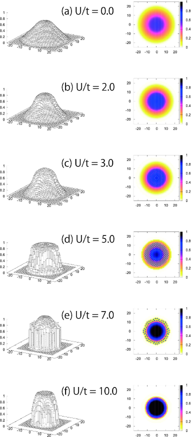
Figure 1: (Color online) The density profile $\langle n_{i\sigma}\rangle$ in the optical lattice system with $d/a=10$ at $T/t=0.05$ when $U/t=0.0,2.0,3.0,5.0,7.0$ and $10.0$ (from the top to the bottom).

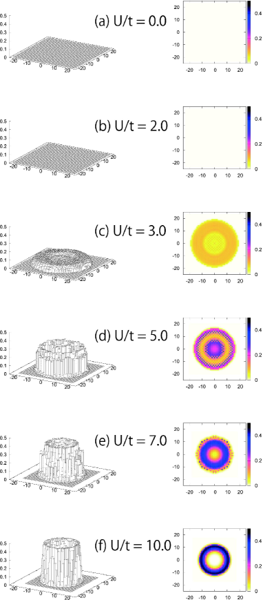
Figure 2: (Color online) The pair potential $\Delta_{i}$ in the optical lattice system with $d/a=10$ at $T/t=0.05$ when $U/t=0.0,2.0,3.0,5.0,7.0$ and $10.0$ (from the top to the bottom).

III Low temperature properties

By means of R-DMFT with the two-site impurity solver, we obtain the results for the system with $d/a=10$ and $N\sim 720(\tilde{\rho}\sim 2.3)$. Figures 1 and 2 show the profiles of the local density and the pair potential at $T/t=0.05$. In the non-interacting case $(U/t=0)$, fermionic atoms are smoothly distributed up to $r/a\sim 21$, as shown in Fig. 1 (a). Increasing the attractive interaction $U$, fermions tend to gather around the bottom of the harmonic potential, as seen in Fig. 1 (b). In these cases, the pair potential is not yet developed, as shown in Figs. 2 (a) and (b), and thereby the normal metallic state with short-range pair correlations emerges in the region ($U/t\lesssim 2$). Further increase in the interaction $U$ leads to different behavior, where the pair potential $\Delta_{i}$ is induced in the region with $\langle n_{i\sigma}\rangle\neq 0$. Thus, the SSF state is induced by the attractive interaction, which is consistent with the results obtained from the Bogoljubov-de Gennes equation FFLO . In the case with $U/t=3$, another remarkable feature is found around the center of the harmonic potential $(r/a<7)$, where a checkerboard structure appears in the density profile $\langle n_{i\sigma}\rangle$, as shown in Fig. 1 (c). This implies that the DW state is realized in the region. On the other hand, the pair potential $\Delta_{i}$ is not suppressed completely even in the DW region, as shown in Fig. 2 (c). This suggests that the DW state coexists with the SSF state, i.e. a supersolid state appears in our optical lattice system. The profile characteristic of the supersolid state is clearly seen in the case of $U/t=5$. Figures 1(d) and 2(d) show that the DW state of checkerboard structure coexists with the SSF state in the doughnut-like region $(5<r/a<15)$. By contrast, the genuine SSF state appears inside and outside of the region $(r/a<5,15<r/a<17)$. Further increase in the interaction excludes the DW state out of the center since fermionic atoms are concentrated around the bottom of the potential for large $U$. In the region, two particles with opposite spins are strongly coupled by the attractive interaction to form a hard-core boson, giving rise to the band insulator with $\langle n_{i\sigma}\rangle\sim 1$, instead of the SSF state. Therefore, the SSF state survives only in the narrow circular region surrounded among the empty and fully occupied states. We see such behavior more clearly in Figs. 1 (f) and 2 (f). Note that in the strong coupling limit $U/t\rightarrow\infty$, all particles are condensed in the region $r<r_{c}=\sqrt{\tilde{\rho}/2}\;d\sim 1.07d=10.7a$.

In this section, we have studied the attractive Hubbard model with the harmonic potential to clarify that the supersolid state is realized in a certain parameter region. However, it is not clear how the supersolid state depends on the system size and the number of particles. To make this point clear, we deal with large clusters to clarify that the supersolid state is indeed realized in the following.

IV Stability of the supersolid state

In this section, we discuss the stability of the supersolid state in fermionic optical lattice systems, which may be important for experimental observations. First, we clarify how low-temperature properties depend on the system size, by performing R-DMFT for several clusters with different $d$. We here fix $U/t=5$ and $\mu/t\sim-1.58$ to obtain the profiles of the local particle density and the pair potential, which are shown in Fig. 3.

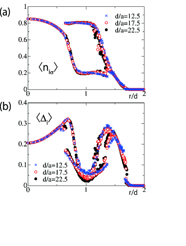
Figure 3: Profiles of particle density $\langle n_{i\sigma}\rangle$ and pair potential $\Delta_{i}$ as a function of $r/d$ with fixed $d=12.5,17.5$ and $22.5$, when $U/t=5$.

We note that the distance $r$ is normalized by $d$ in the figure. It is found that $\langle n_{i\sigma}\rangle$ and $\Delta_{i}$ describe smooth curves for $r/d\lesssim 0.6$ and $1.4\lesssim r/d\lesssim 1.7$, where the genuine SSF state is realized. On the other hand, for $0.6\lesssim r/d\lesssim 1.4$, two distinct magnitudes appear in $\langle n_{i\sigma}\rangle$, reflecting the fact that the DW state with two sublattices is realized. Since the pair potential is also finite in the region, the supersolid state is realized. In this case, we deal with finite systems, and thereby all data are discrete in $r$. Nevertheless, it is found that the obtained results are well scaled by $d$ although some fluctuations appear due to finite-size effects in the small $d$ case. The effective particle density $\tilde{\rho}$ is almost constant in the above cases. Therefore, we conclude that when $\tilde{\rho}\sim 2.3$, the supersolid state discussed here is stable in the limit with $N,d\rightarrow\infty$. This result does not imply that the supersolid state is realized in the homogeneous system with arbitrary fillings. In fact, the supersolid state might be realizable only at half filling Scalettar ; Freericks ; Capone ; Garg ; Micnas . Therefore, we can say that a confining potential is essential to stabilize the supersolid state in the optical lattice system.

Next, we focus on the system with $U/t=5$ and $d/a=10$ to discuss in detail how the supersolid state depends on the effective particle density $\tilde{\rho}$. The DW state is characterized by the checkerboard structure in the density profile $\langle n_{i\sigma}\rangle$, so that the Fourier transform $n_{q}$ at $q=(\pi,\pi)$ is appropriate to characterize the existence of the DW state. On the other hand, the Fourier transform $\Delta_{q}$ at $q=(0,0)$ may represent the rigidity of the SSF state in the system.

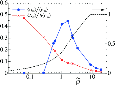
Figure 4: (Color online) $\langle n_{\pi\pi}\rangle/\langle n_{00}\rangle$ and $\Delta_{00}/5\langle n_{00}\rangle$ as a function of the effective particle density $\tilde{\rho}(=N/\pi d^{2})$ when $U=5t$ and $T=0.05t$. A broken line represents the local particle density at the center of the lattice in the noninteracting case.

In Fig. 4, we show the semilog plots of the parameters normalized by $\langle n_{00}\rangle$. It is found that the normalized parameter $\Delta_{00}$ is always finite although the increase in the attractive interaction monotonically decreases it. This implies that the SSF state appears in the system with the arbitrary particle number. In contrast to this SSF state, the DW state is sensitive to the effective particle density as shown in Fig. 4. These may be explained by the fact that in the system without a harmonic confinement $(V_{0}=0)$, the DW state is realized only at half filling $(n=0.5)$, while the SSF state is always realized. To clarify this, we also show the local particle density in the noninteracting case at the center of the system as the broken line in Fig. 4. It is found that when the quantity approaches half-filling $(\sim 0.5)$, $\langle n_{\pi\pi}\rangle/\langle n_{00}\rangle$ takes its maximum value, where the SSF state coexists with the DW state. Therefore, we can say that the supersolid state is stable around this condition. Increasing the effective particle density, the band insulating states become spread around the center, while the DW and SSF states should be realized in a certain circular region surrounded among the empty and fully-occupied regions. Therefore, the normalized parameters $\langle n_{\pi\pi}\rangle$ and $\Delta_{00}$ are decreased with increase in $\tilde{\rho}$. On the other hand, in the case with low density $\tilde{\rho}\lesssim 0.3$, the local particle density $n_{i}$ at each site is far from half filling even when $U/t=5$. Therefore, the DW state does not appear in the system, but the genuine SSF state is realized. These facts imply that the condition $n\sim 0.5$ is still important to stabilize the supersolid state even in fermionic systems confined by a harmonic potential.Pour

By performing similar calculations for the systems with low, intermediate, and high particle densities ($\tilde{\rho}\sim 0.63,2.3$ and $8.9$), we end up with the phase diagrams, as shown in Fig. 5.

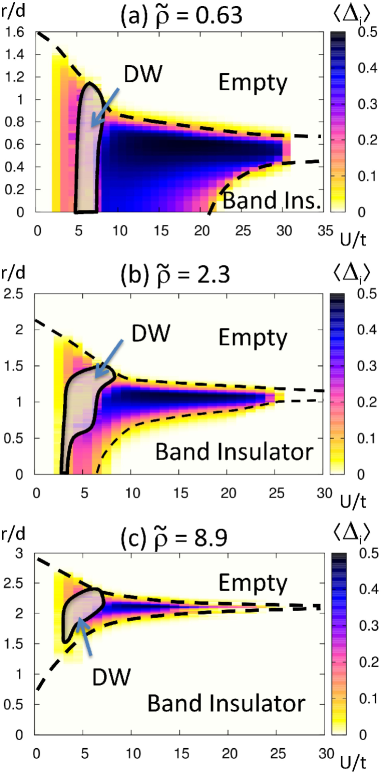
Figure 5: (Color online) The phase diagram of the attractive Hubbard model on the optical lattice with $\tilde{\rho}\sim 0.63,2.3$ and $8.9$. The density plot represents the profiles of the $s$-wave pair potential as a function of the attractive interaction $U/t$. The DW state is realized in the shaded area. The broken lines give a guide to eyes which distinguishes the region with a fractional particle density from the empty and fully-occupied regions.

We find that increasing the attractive interaction, fermionic particles gradually gather around the center of the system, where the empty state is stabilized away from the center and the band insulating state with fully occupied sites is stabilized. It is found that the region surrounded among these states strongly depend on the effective particle density $\tilde{\rho}$. The increase in the effective particle density shrinks the region, which affects the stability of the SSF, DW and their coexisting states. In particular, the DW region, which is shown as the shaded area in Fig. 5, is sensitive to the effective particle density, as discussed above. Namely, the local pair potential $\Delta_{i}$ takes its maximum value around $U/t\sim 15$, which may give a rough guide for the crossover region between the BCS-type and the BEC-type states. We note that the DW state appears only in the BCS region $(U/t\sim 5)$. This implies that the condition $n\sim 0.5$ is not sufficient, but necessary to stabilize the supersolid state in the attractive Hubbard model with an inhomogeneous potential.

We wish to comment on the conditions to observe the supersolid state in the fermionic optical lattice system. Needless to say, one of the most important conditions is the low temperature.Koga Second is the tuning of the effective particle density $\tilde{\rho}(\sim 1)$, which depends on the curvature of the harmonic potential as well as the total number of particles. This implies that a confined potential play a crucial role in stabilizing the supersolid state in fermionic optical lattice systems. In addition to this, an appropriate attractive interaction is necessary to stabilize the DW state in the BCS-type SSF state. When these conditions are satisfied, the supersolid state is expected to be realized at low temperatures.

V Summary

We have investigated the fermionic attractive Hubbard model in the optical lattice with harmonic confinement. By combining R-DMFT with a two-site impurity solver, we have obtained the rich phase diagram on the square lattice, which has a remarkable domain structure including the SSF state in the wide parameter region. By performing systematic calculations, we have then confirmed that the supersolid state, where the SSF state coexists with the DW state, is stabilized even in the limit with $N\rightarrow\infty,V_{0}\rightarrow 0$ and $\tilde{\rho}\sim$ const. We have also elucidated that a confining potential plays a key role in stabilizing the supersolid state.

- (1) M. H. Anderson, J. R. Ensher, M. R. Matthews, C. E. Wieman, and E. A. Cornell: Science 269 (1995) 198.
- (2) For a review, see Nature (London) 416 (2002) 205-246.
- (3) C. J. Pethick and H. Smith, Bose-Einstein Condensation in Dilute Gases (Cambridge University Press, Cambridge, 2002).
- (4) L. Pitaevskii and S. Stringari, Bose-Einstein Condensation (Clarendon Press, Oxford, 2003).
- (5) I. Bloch and M. Greiner: Advances in Atomic, Molecular, and Optical Physics, edited by P. Berman and C. Lin (Academic Press, New York, 2005), Vol. 52 p. 1.
- (6) I. Bloch: Nature Physics 1 (2005) 23.
- (7) D. Jaksch and P. Zoller: Ann. Phys. (NY) 315 (2005) 52.
- (8) O. Morsch and M. Oberhaler: Rev. Mod. Phys. 78 (2006) 179.
- (9) M. Greiner, O. Mandel, T. Esslinger, T. W. Hänsch and I. Bloch: Nature 415 (2003) 39.
- (10) J. K. Chin, D. E. Miller, Y. Liu, C. Stan, W. Setiawan, C. Sanner, K. Xu, and W. Ketterle: Nature 443 (2006) 961.
- (11) R. Jördens, N. Strohmaier, K. Günter, H. Moritz, T. Esslinger, arXiv:0804.4009.
- (12) U. Schneider, L. Hackermüller, S. Will, Th. Best, I. Bloch, T. A. Costi, R. W. Helmes, D. Rasch and A. Rosch, arXiv:0809.1464.
- (13) E. Kim and M. H. W. Chan: Nature 427 (2004) 225.
- (14) P. Sengupta, L. P. Pryadko, F. Alet, M. Troyer, and G. Schmid: Phys. Rev. Lett. 94 (2005) 207202; D. L. Kovrizhin, G. V. Pai, and S. Sinha: Europhysics Letters 72 (2005) 162; V. W. Scarola and S. Das Sarma: Phys. Rev. Lett. 95 (2005) 033003; S. Wessel and M. Troyer: Phys. Rev. Lett. 95 (2005) 127205; D. Heidarian and K. Damle: Phys. Rev. Lett. 95 (2005) 127206; R. G. Melko, A. Paramekanti, A. A. Burkov, A. Vishwanath, D. N. Sheng, and L. Balents: Phys. Rev. Lett. 95 (2005) 127207; G. G. Batrouni, F. Hébert, and R. T. Scalettar: Phys. Rev. Lett. 97 (2006) 087209.
- (15) H. P. Büchler and G. Blatter: Phys. Rev. Lett. 91 (2003) 130404; I. Titvinidze, M. Snoek and W. Hofstetter: Rhys. Rev. Lett., 100, 100401 (2008).
- (16) R. T. Scalettar, E. Y. Loh, J. E. Gubernatis, A. Moreo, S. R. White, D. J. Scalapino, R. L. Sugar, and E. Dagotto: Phys. Rev. Lett. 62 (1989) 1407.
- (17) J. K. Freericks, M. Jarrell, and D. J. Scalapino: Phys. Rev. B 48 (1993) 6302.
- (18) F. Karim Pour, M. Rigol, S. Wessel, and A. Muramatsu, Phys. Rev. B 75, 161104(R) (2007).
- (19) A. Koga, T. Higashiyama, K. Inaba, S. Suga, and N. Kawakami, J. Phys. Soc. Jpn. 77, 073602 (2008).
- (20) M. Capone, C. Castellani, and M. Grilli: Phys. Rev. Lett. 88 (2002) 126403.
- (21) R. Micnas, J. Ranninger, and S. Robaszkiewicz: Rev. Mod. Phys. 62 (1990) 113.
- (22) M. Keller, W. Metzner, and U. Schollwöck: Phys. Rev. Lett. 86 (2001) 4612.
- (23) A. Garg, H. R. Krishnamurthy, and M. Randeria: Phys. Rev. B 72 (2005) 024517.
- (24) A. Toschi, M. Capone, and C. Castellani: Phys. Rev. B 72 (2005) 235118.
- (25) Y. Chen, Z. D. Wang, F. C. Zhang, and C. S. Ting: cond-mat/0710. 5484.
- (26) M. Yamashita and M. W. Jack: Phys. Rev. A76 (2007) 023606.
- (27) A. Rüegg, S. Pilgram, and M. Sigrist: Phys. Rev. B 75 (2007) 195117.
- (28) Y. Fujihara, A. Koga, and N. Kawakami: J. Phys. Soc. Jpn. 76 (2007) 034716.
- (29) T.-L. Dao, A. Georges, and M. Capone: arXiv:0704.2660.
- (30) M. Machida, S. Yamada, Y. Ohashi, and H. Matsumoto: Phys. Rev. A 74 (2006) 053621.
- (31) M. Rigol, A. Muramatsu, G. G. Batrouni, and R. T. Scalettar: Phys. Rev. Lett. 91 (2003) 130403.
- (32) W. Metzner and D. Vollhardt: Phys. Rev. Lett. 62 (1989) 324; E. Müller-Hartmann: Z. Phys. B 74 (1989) 507; T. Pruschke, M. Jarrell, and J. K. Freericks: Adv. Phys. 42 (1995) 187; A. Georges, G. Kotliar, W. Krauth and M. J. Rozenberg: Rev. Mod. Phys. 68 (1996) 13.
- (33) M. Potthoff and W. Nolting: Phys. Rev. B 59 (1999) 2549.
- (34) S. Okamoto and A. J. Millis: Phys. Rev. B 70 (2004) 241104(R); Nature (London) 428 (2004) 630.
- (35) R. W. Helmes, T. A. Costi and A. Rosch: Phys. Rev. Lett. 100 (2008) 056403.
- (36) M. Snoek, I. Titvinidze, C. Töke, K. Byczuk, and W. Hofstetter: arXiv:0802.3211.
- (37) G. Xianlong, M. Rizzi, M. Polini, R. Fazio, M. P. Tosi, V. L. Campo Jr. and K. Capelle, Phys. Rev. Lett. 98, 030404 (2007).
- (38) T. Higashiyama, K. Inaba, and S. I. Suga, Phys. Rev. A 77, 043624 (2008).
- (39) M. Potthoff: Phys. Rev. B 64 (2001) 165114.