RooStatsCms: a tool for analyses modelling, combination and statistical studies.

Abstract

The RooStatsCms (RSC) software framework allows analysis modelling and combination, statistical studies together with the access to sophisticated graphics routines for results visualisation. The goal of the project is to complement the existing analyses by means of their combination and accurate statistical studies.

Soon the LHC machine will open a new exciting era of measurement campaigns. A reliable and widely accepted tool for analyses combination and statistical studies is needed at first for limits estimations. Then it should provide the basis for discoveries and finally parameter measurements. Our proposed solution is RooStatsCms [1].

1 Statistical methods

1.1 Separation of signal plus background and background only hypotheses

The analysis of search results can be formulated in terms of a hypothesis test. The first step consists in identifying the observables which comprise the results, e.g. the number of signal events observed or the cross section for a particular process. Then a test statistic is specified. A good choice is $Q^{\prime}=-2\ln Q$, where $Q=L_{1}/L_{0}$ and $L_{0}$ and $L_{1}$ are, for a given dataset, the likelihoods computed in the $\mathcal{H}_{0}$ (background only, b) and $\mathcal{H}_{1}$ (signal plus background, sb) hypotheses respectively. The last step is to define rules for discovery and exclusion. In [2] is proposed the $CL_{s}=CL_{sb}/CL_{b}$ quantity value, where

$$CL_{sb}=P_{sb}(Q\leq Q_{obs})=\int^{Q_{obs}}_{-\infty}\frac{dP_{sb}}{dQ}dQ$$ (1)

and

$$CL_{b}=P_{b}(Q\leq Q_{obs})=\int^{Q_{obs}}_{-\infty}\frac{dP_{b}}{dQ}dQ.$$ (2)

The quantity $\frac{dP_{sb}}{dQ}$ is the probability density function of the test statistic in the sb experiments (see Fig. 1). The 95% confidence level (CL) exclusion of the signal hypothesis is usually quoted in case of a $CL_{s}\leqslant 5\%$.

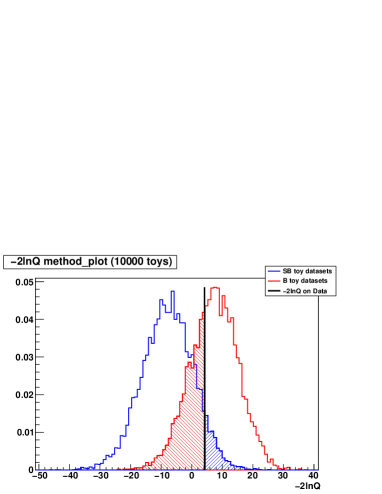
Figure 1: The distributions of $-2\ln Q$ in the background only (red, on the right) and signal plus background (blue, on the left) hypotheses. The black line represents the value of $-2\ln Q$ on the measured data. The shaded areas represent $1-CL_{b}$ (red) and $CL_{sb}$ (blue). The $-2\ln Q$ variable can be used instead of $Q$ to ease the calculations without any loss of generality.

1.2 Profile likelihood (PL)

Suppose to have the Likelihood function $L(\underline{x},\underline{\theta})$, where $\underline{x}$ are the quantities measured for each event and $\underline{\theta}$ the $K$ parameters of the joint pdf describing the data [3]. The idea of the PL technique is to select a parameter $\theta_{0}$ and perform a scan over a sensible range of values. For every point of the scan, the value of $\theta_{0}$ is fixed and the quantity $-\ln L$ ($nll$) is maximised with respect to the remaining $K$-1 $\theta_{i}$ parameters. The values are then plotted versus $\theta_{0}$ (Fig. 2). Without any loss of generality, the negative loglikelihood scan is usually considered in terms of $\Delta nll$, with its minimum value equal to 0: this is always possible with a shift of all the scan points. This curve minimum point abscissa represents the maximum likelihood estimator for $\theta_{0}$, $\hat{\theta}_{0}$. Finally, upper limits and intervals of a given CL can be read simply from the PL curve, tracing horizontal lines at predefined vertical values [4].

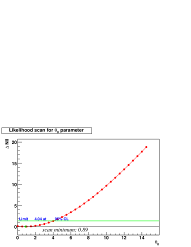
Figure 2: The Likelihood scan in terms of $\Delta nll$ and the horizontal line for the 95% CL upper limit ($\Delta nll\simeq 1.36$). The interpolation between scan point pairs is linear, while the minimum of the scan is the minimum of a parabola built on the lowest three points.

2 The RSC framework

Based on the RooFit [5] technology, RSC is composed of three parts: the analysis modelling and combination, the implementation of statistical methods and sophisticated graphics routines for results visualisation. This framework is intended to be a product for the CMS collaboration but a public version, which does not include the modelling part, is available under the name of RooStatsKarlsruhe [6].

All the RSC classes inherit from the ROOT [7] TObject. In this way it is possible to prototype very quickly macros to be run interactively and all the RSC objects can be written on disk in rootfiles exploiting the persistency mechanism implemented by ROOT.

The analyses and their combinations are described in ASCII configuration files in the “ini” format: the datacards. The user at first specifies the observable(s) involved in the analysis. Thus the signal and background components relative to the observable(s) are characterised: the framework also allows to consider multiple components for one single observable. The single components can be the result of a counting analysis or be represented by shapes. Both cases can be taken into account and in presence of a shape, the user can decide to describe it through a parametrisation or to read it directly from a ROOT histogram stored in a rootfile. The yields of the components can be described as a single quantity or as a product of many factors, e.g. $yield=\mathcal{L}\cdot\sigma_{production}\cdot BR\cdot\epsilon$: the product of the integrated luminosity, the production cross section, the branching ratio and the cuts efficiency. The systematics on all the the parameters present in the model description together with their correlations can also be described in the datacard.

The construction of the RooFit objects representing the (combined) analyses is performed through the parsing and processing of the datacard. This approach has two advantages: it factorises the analysis description from the actual statistical studies and provides to the analyses groups a common base to share their results.

The calculations implied by certain statistical methods may be very CPU-intensive, e.g. if the execution of many Monte Carlo toy experiments is foreseen. The RSC classes that implement those methods are designed to ease the creation of multiple jobs intended for a batch system or the grid. The outcome is collected in results objects which can be written on disk: to every statistical method class corresponds a results class. Such objects can be recollected and added together therewith profiting from a very high Monte Carlo toy experiments statistic.

Special care was devoted to the display of the results: for every results class, a plot class is implemented. Therefore in the final step of a statistical study the user can get a plot object out of a results object and draw it. These two last operations are straightforward and need only two lines of C++ code to be carried out. In addition to the plots directly linked to the results, RSC gives the possibility to build other widely accepted plots (see Fig. 3) with standalone classes. Examples of plots produced with RSC are Fig. 1, Fig. 2, Fig. 3.

A big effort was dedicated to the RSC documentation and examples. All the classes, methods, members and namespaces are provided with Doxygen style comments and a website of RooStatsCms is available [1]. A wikipage is also present in the official CMS wiki . The framework is distributed with example ROOT macros, C++ programs ready to be compiled and Python scripts to ease the creation of the datacards.

A possible application of the RSC implementation of the statistical methods described in 1.1 and 1.2 is discussed in section 3.

3 A concrete application

For the the CMS VBF $H\rightarrow\tau\tau$ analysis ($1~{}fb^{-1}$) [8] study, RSC was used. Given the disadvantageous $s/b$ ratio in the various mass hypotheses with this integrated luminosity, we put an exclusion limit on the H boson production cross section using the technique described in section 1.1. Fig. 3 shows the expected $H$ production cross section ($\sigma$) that could be excluded with the data available, i.e. the Monte Carlo (MC) statistic available after all the cuts, in units of Standard Model (SM) $\sigma$. To derive the shape of the $\frac{dP}{dQ}$ pdf for the two hypotheses several toy MC experiments were performed.

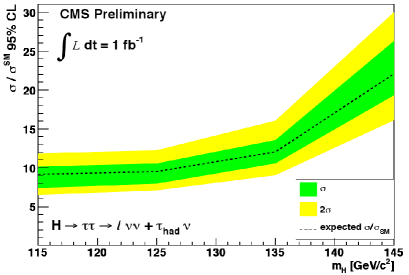
Figure 3: Exclusion plot for the VBF $H\rightarrow\tau\tau$ CMS analysis. The 1$\sigma$ and 2$\sigma$ bands are obtained assuming to observe a 1$\sigma$ or 2$\sigma$ upwards (downwards) fluctuation of the number of observed background events. The plot is produced with a graphics class of RSC.

To take into account the systematics, before the generation of each toy MC dataset, the parameters values affected by systematic uncertainties were fluctuated according to their expected distribution, assumed in this case Gaussian.

Performing several toy MC experiments we derived also the distribution of the upper limits at 95% confidence level shown in Fig. 4 focusing on the number of signal events ($N_{s}$). In this second study systematic uncertainties were not considered.

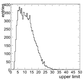
Figure 4: The distribution of the 95% CL upper limits on the number of signal events for $m_{H}=145$ GeV. The median is located at $10.71$ signal events which corresponds to a $\sigma/\sigma_{SM}$ equal to $6.7$.

An analysis of the coverage, i.e. the fraction of cases in which the upper limit is indeed greater than the nominal $N_{s}$, was carried out (Fig. 5). The $N_{s}$ value was also artificially incremented in order to study the coverage at different working points. Overcoverage is present for low signal yields leading to conservative upper limits. This feature can be seen as a consequence of the Cramér-Fréchet inequality [4].

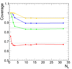
Figure 5: The coverage in case of 68%, 84%, 90%, 95% CL (coloured lines) versus nominal $N_{s}$. The reference coverages are shown with the dashed lines.

4 Conclusions

Two statistical analyses were carried out using the RSC framework. The hypotheses separation study shows that it is possible to compute exclusion limits in the context of a hypothesis separation test by means of the integrals of the discriminating variables pdf. The PL method can be used as well for extracting upper limits but it was verified that a significant overcoverage occurs in case of very small quantities.

The RooStatsCms proved to be a reliable and valuable tool for analyses modelling and complex statistical procedures deployment in a simple and flexible way. The graphical routines embedded in the package serve as a powerful tool for results visualisation.

References

- [1] D. Piparo, G. Schott, G. Quast “RooStatsCms: a tool for analyses modelling, combination and statistical studies”, CMS note (in preparation), www-ekp.physik.uni-karlsruhe.de/~RooStatsCms.
- [2] A.L. Read “Modified frequentist analysis of search results (The method)”, CERN open-2000-205.
- [3] F. James “Statistical in Experimental Physics 2nd Edition”, Word Scientific 2006.
- [4] W.J. Metzger “Statistical Methods in Data Analysis”, Katholieke Universiteit Nijmegen, 2002.
- [5] W. Verkerke, D. Kirkby “The RooFit toolkit for data Modelling”, roofit.sourceforge.net.
- [6] D. Piparo, G. Schott, G. Quast “RooStatsKarlsruhe”, www-ekp.physik.uni-karlsruhe.de/~RooStatsKarlsruhe
- [7] ROOT: An Object Oriented Data Analysis Framework, root.cern.ch.
- [8] CMS Collaboration, CMS PAS HIG 08-008.