Lattice cutoff effects for $F_{\rm D_{s}}$ with improved Wilson fermions – a final lesson from the quenched case

Abstract:

In view of the recent excitement about a tension between determinations of $F_{\rm D_{s}}$ from experiment and from simulations of lattice QCD with dynamical quarks, we try to clear up the picture of lattice determinations in the continuum limit of the quenched approximation. For ${\rm O}(a)$ improved Wilson quarks we see linear scaling in the squared lattice spacing $a^{2}$ only for $a\lesssim 0.08\,$fm. For coarser lattices we observe significant contaminations from higher order cutoff effects. As an aside we also study the scaling of the charm quark mass and the ratio of the vector to the pseudo-scalar decay constant and the spin-splitting.

1 Introduction

Since the time when simulations of lattice QCD with dynamical fermions became feasible, the phenomenology of the ${\rm D_{s}}$-meson has been considered as a field where lattice QCD could provide benchmark predictions that would be confronted with increasingly precise measurements from experiments like Belle, BaBar and CLEO-c. Preparatory tests of the techniques in quenched lattice QCD [1, 2] indicated that a precision of only a few percent for observables like $F_{\rm D_{s}}$ is possible when simulating the full theory, while keeping all sources of systematic uncertainties under control.

Only recently, precise determinations of $F_{\rm D_{s}}$ appeared in dynamical simulations with $N_{\rm f}=2$ and 2+1 flavours of sea quarks [3, 4, 5, 6]. The central values, although partly preliminary [5, 6], turned out to be about 10% larger than in the quenched case. This was not surprising given that the quenching error was always estimated to lie in the range of 10–20%. Surprising, however, turned out to be a recent comparison with a compilation of experimental results for $F_{\rm D_{s}}$ [7] by CLEO-c [8] and Belle [9, 10]. A tension between the experimental value and lattice results triggered speculations about possible signs for physics beyond the Standard Model [11].

In this work we want to emphasize that the lattice spacing dependence must be mapped out over a large range in order to unambiguously isolate the leading lattice artefacts – this is all the more important in the heavy quark sector. In particular the approach to the continuum limit of the leptonic decay constant of the ${\rm{D}_{s}}$-meson in the quenched approximation, as recently summarized in [2, 12], did not exhibit proper scaling, and we try to clarify this issue here. It appears that simulations with lattice spacings larger than $a\approx 0.08\,$fm can suffer from ambiguities in the ${\rm O}(a)$ improvement of the quark bilinear currents, which significantly affects the extrapolation of the data to the continuum limit. It is indispensable to go to smaller lattice spacings in order to assure scaling. These findings are extremely important for assessing current error estimates in lattice studies of $F_{\rm D_{s}}$ in the unquenched case as they have been reported by ALPHA, ETMC, HPQCD and MILC [6, 5, 4, 3].

To this end we extend the ALPHA Collaboration’s computation of $F_{\rm D_{s}}$ in the quenched approximation reported in [1] for lattice spacings in the range $a\approx 0.09-0.05\,$fm by simulations of an additional lattice spacing $a\approx 0.03\,$fm [13]. Moreover, we increased the statistics with respect to [1] and [13] significantly, which allows us to present a comprehensive picture of the lattice spacing dependence of the decay constant $F_{\rm D_{s}}$ in quenched lattice QCD with non-perturbatively improved Wilson quarks. In addition, we also present scaling studies for the renormalization group invariant charm quark mass $M_{\rm c}$ [14, 13], the mass splitting $m_{{\rm{D}_{s}^{\ast}}}-m_{{\rm{D}_{s}}}$ and of the ratio of the vector to pseudo-scalar meson decay constants $F_{\rm D_{s}^{\ast}}/F_{\rm D_{s}}$ [13]. We start by briefly explaining the setup of our large-volume simulations of the quenched QCD Schrödinger functional [15, 16] and then discuss the simulation parameters. This is succeeded by a presentation of our results, before ending with a discussion and our conclusion.

2 Details of the simulation

In the following we introduce the set of Schrödinger functional correlation functions, from which we determine ${m_{\rm{D}_{s}}}$, ${m_{\rm{D}_{s}^{\ast}}}$, $F_{\rm D_{s}}$, $F_{\rm D_{s}^{\ast}}$ and the mass of the charm quark. We compute the correlation functions directly for all required mass-degenerate and non-degenerate combinations built from quark propagators at the physical strange quark mass and at two values of the charm quark mass close to the physical one. This allows for an interpolation of the results to the exact physical point, which we define through the experimentally determined mass of the ${\rm{D}_{s}}$-meson as input. This computation is repeated for five different lattice spacings in the range of $a\approx 0.1-0.0\,3\,$fm in order to investigate the scaling behaviour of our observables and identify a range in the lattice spacing where observables scale linearly in $a^{2}$.

2.1 Correlation functions

For this study the relevant Schrödinger functional heavy-light 2-point correlation functions are

$$\begin{array}[]{l}f_{\rm A}(x_{0})=-\frac{1}{2}\langle A_{0}(x){\cal O}\rangle\,,\ \ f_{\rm P}(x_{0})=-\frac{1}{2}\langle P(x){\cal O}\rangle\,,\ \ f_{1}=-\frac{1}{2L^{6}}\langle{\cal O}^{\prime}{\cal O}\rangle\,,\\[5.69054pt] f_{\rm V}(x_{0})=-\frac{1}{6}\sum\limits_{i}\langle V_{i}(x){\cal O}_{i}\rangle\,,\ \ f_{{\rm T},\mu}(x_{0})=-\frac{1}{6}\sum\limits_{i}\langle T_{\mu i}{\cal O}_{i}(x)\rangle\,,\ \ k_{1}=-\frac{1}{6L^{6}}\sum\limits_{i}\langle{\cal O}^{\prime}_{i}{\cal O}_{i}\rangle\,,\end{array}$$ (1)

where $A_{\mu}(x)=\overline{\psi}_{\rm s}(x)\gamma_{\mu}\gamma_{5}\psi_{\rm h}(x)$ is the axial-vector current, $P(x)=\overline{\psi}_{\rm s}(x)\gamma_{5}\psi_{\rm h}(x)$ is the pseudo-scalar density, and $V_{\mu}(x)=\overline{\psi}_{\rm s}(x)\gamma_{\mu}\psi_{\rm h}(x)$ and $T_{\mu\nu}(x)=\overline{\psi}_{\rm s}(x)\sigma_{\mu\nu}\psi_{\rm h}(x)$ are the vector and tensor currents. In each case we indicate the respective quark flavour with a subscript “${\rm s}$” for light ($=$ strange) and “${\rm h}$” for heavy quarks with masses close to the one of the charm quark. The quark bilinears

$${\cal O} = \frac{a^{6}}{L^{3}}\sum_{{\bf y},{\bf z}}\overline{\zeta}_{\rm h}({\bf y})\gamma_{5}\zeta_{\rm s}({\bf z})\,,\quad{\cal O}^{\prime}=\frac{a^{6}}{L^{3}}\sum_{{\bf y},{\bf z}}\overline{\zeta}^{\prime}_{\rm s}({\bf y})\gamma_{5}\zeta^{\prime}_{\rm h}({\bf z})\,,$$ (2)

$${\cal O}_{i} = \frac{a^{6}}{L^{3}}\sum_{{\bf y},{\bf z}}\overline{\zeta}_{\rm h}({\bf y})\gamma_{i}\zeta_{\rm s}({\bf z})\,,\quad{\cal O}^{\prime}_{i}=\frac{a^{6}}{L^{3}}\sum_{{\bf y},{\bf z}}\overline{\zeta}^{\prime}_{\rm s}({\bf y})\gamma_{i}\zeta^{\prime}_{\rm h}({\bf z})\,,$$ (3)

are the meson wall sources at the $x_{0}=0$ and the $x_{0}=T$ boundary timeslices, respectively. For more details on Schrödinger functional correlation functions and for unexplained notation we refer the reader to, e.g., refs. [17, 18]. We employ the improved axial-vector and vector currents

$$A_{0}^{\rm I}(x)=A_{0}(x)+c_{\rm A}a\tilde{\partial}_{0}P(x)\quad{\rm and}\quad V_{i}^{\rm I}(x)=V_{i}(x)+c_{\rm V}a\tilde{\partial}_{0}T_{0i}(x)\,,$$ (4)

where $\tilde{\partial}_{0}$ is the time component of the symmetrized next-neighbour lattice derivative. The improvement coefficients $c_{\rm A}(g_{0})$ and $c_{\rm V}(g_{0})$ for the quenched theory have been determined non-perturbatively in [19] and [20, 21], respectively. On the lattice, the axial-vector current and the vector current receive a multiplicative (scale independent) renormalization and we write

$$(A_{\rm R})_{0}=Z_{\rm A}\left[1+b_{\rm A}(am_{{\rm q},{\rm h}}+am_{{\rm q},{\rm s}})/2\right]A_{0}^{\rm I}+{\rm O}(a^{2})\,,$$ (5)

$$(V_{\rm R})_{i}=Z_{\rm V}\left[1+b_{\rm V}(am_{{\rm q},{\rm h}}+am_{{\rm q},{\rm s}})/2\right]V_{i}^{\rm I}+{\rm O}(a^{2})\,.$$ (6)

The corresponding renormalization constants for the quenched theory $Z_{\rm A}(g_{0})$ and $Z_{\rm V}(g_{0})$ have been determined non-perturbatively in [23]. ${\rm O}(a)$ artifacts that are proportional to the bare subtracted quark masses $am_{{\rm q},i}=\frac{1}{2}\big{(}\frac{1}{\kappa_{i}}-\frac{1}{\kappa_{\rm crit}}\big{)}$ for $i={\rm s},{\rm h}$, where $\kappa_{\rm crit}$ is the critical hopping parameter, are canceled by terms proportional to the improvement coefficients $b_{\rm A}(g_{0})$ and $b_{\rm V}(g_{0})$; they have been calculated in 1-loop perturbation theory [20].

2.2 Observables

We define the pseudo-scalar effective mass via

$$am_{\text{PS}}(x_{0}+a/2)=\log\frac{f_{\rm A}^{\rm I}(x_{0})}{f_{\rm A}^{\rm I}(x_{0}+a)}\,,$$ (7)

and the expression for the local pseudo-scalar meson decay constant is given by [18]

$$a{F_{\rm PS}}(x_{0}) = -2Z_{\rm A}\left[1+b_{\rm A}(am_{{\rm q},{\rm h}}+am_{{\rm q},{\rm s}})/2\right]\frac{f_{\rm A}^{\rm I}(x_{0})}{\sqrt{f_{1}}}\,(m_{\rm PS}L^{3})^{-1/2}\,{\rm e}^{\,(x_{0}-T/2)m_{\rm PS}}$$ (8)

$$\times\left\{1-\eta_{\rm A}^{\rm PS}{\rm e}^{\,-x_{0}\Delta}-\eta_{\rm A}^{0}{\rm e}^{\,-(T-x_{0})m_{\text{G}}}\right\}+{\rm O}(a^{2})\,,$$

and an analogous expression holds for the mass and the decay constant in the vector channel. In (8) the factor $(m_{\rm PS}L^{3})^{-1/2}$ takes into account the normalization of one-particle states, and $f_{1}^{-1/2}$ cancels out the dependence on the meson sources. Because of its exponential decay, the correlation function $f_{\rm A}^{\rm I}$ is dominated by the ground state in the pseudo-scalar channel for large time separations from the boundaries (i.e. $x_{0}$ and $T-x_{0}$). Hence, eqs. (7) and (8) are expected to exhibit a plateau at intermediate times, when the contribution $\eta_{\rm A}^{\rm PS}{\rm e}^{\,-x_{0}\Delta}$ of the first excited state and the contribution $\eta_{\rm A}^{0}{\rm e}^{\,-(T-x_{0})m_{\text{G}}}$ from the $O^{++}$ glueball both are small and well below the statistical errors, such that final estimates for masses and decay constants are obtained by fits to a constant within the plateau regions of the local quantities (7) and (8), as explained in [18].

Concerning the quark masses, we employ the continuum PCAC relation, which in the situation of QCD with non-degenerate quarks at hand can be written as

$$\partial_{\mu}A_{\mu}(x)=2m_{\rm hs}P(x)=(m_{\rm hh}+m_{\rm ss})P(x)$$ (9)

and on the lattice translates into a definition of the bare current quark mass in terms of the heavy-light correlation functions (1) [17],

$$am_{\rm hs}(x_{0})=\frac{a}{2}\left[{\frac{1}{2}}(\partial^{\ast}_{0}+\partial_{0})f_{\rm A}(x_{0})+c_{\rm A}a\partial_{0}^{\ast}\partial_{0}f_{\rm P}(x_{0})\right]/f_{\rm P}(x_{0})\,,$$ (10)

$\partial_{0}$ ($\partial^{\ast}_{0}$) being the forward (backward) lattice derivative in the time direction. In this notation, a single quark mass $m_{ii}$, $i={\rm s},{\rm h}$, is obtained if the quark flavours are mass degenerate. Again it is understood that the bare heavy-light current quark masses entering the formulae below are computed as timeslice averages within a central flat region of the associated local masses, eq. (10).

After multiplicative renormalization of the improved axial current and the pseudo-scalar density we obtain the identity

$$\begin{array}[]{rcl}a(m_{{\rm R},{\rm h}}+m_{{\rm R},{\rm s}})&=&\displaystyle 2\,\frac{Z_{\rm A}\left[1+b_{\rm A}{\frac{1}{2}}(am_{{\rm q},{\rm h}}+am_{{\rm q},{\rm s}})\right]}{Z_{\rm P}\left[1+b_{\rm P}{\frac{1}{2}}(am_{{\rm q},{\rm h}}+am_{{\rm q},{\rm s}})\right]}\,am_{\rm hs}+{\rm O}(a^{2})\\ \\ &=&2Z_{\rm A}Z_{\rm P}^{-1}\left[1+(b_{\rm A}-b_{\rm P}){\frac{1}{2}}(am_{{\rm q},{\rm h}}+am_{{\rm q},{\rm s}})\right]am_{\rm hs}+{\rm O}(a^{2})\end{array}$$ (11)

for the sum of the renormalized PCAC heavy and strange (valence) quark masses in the O($a$) improved theory, where $(b_{\rm A}-b_{\rm P})(g_{0})$ has been determined non-perturbatively in [24]. The scale dependent (and, in quark mass independent renormalization schemes, also flavour independent) renormalization factor $Z_{\rm P}=Z_{\rm P}(g_{0},L/a)$ encodes the scale dependence of the renormalized quark masses and is available from [25] in the Schrödinger functional scheme for $N_{\rm f}=0$ and the range of bare couplings relevant here. Eventually, using the flavour independent ratio $M/m_{{\rm R},i}(\mu)$, $\mu=1/L$, in the continuum limit, we combine this with $Z_{\rm A}/Z_{\rm P}$ into the total renormalization factor $Z_{\rm M}(g_{0})$ [25] to express our results directly in terms of the scale and scheme independent renormalization group invariant (RGI) quark mass $M$. The RGI mass is very convenient since it may then be straightforwardly converted to any other renormalization scheme, such as $\overline{{\rm MS}}$ at some desired scale, by means of continuum perturbation theory.

From the various quark mass definitions for non-degenerate and degenerate quarks we construct the following expressions for the O($a$) improved RGI heavy (i.e. charm) quark mass. Once we compute it via the current quark mass from the heavy-strange current with the strange current quark mass subtracted,

$$\begin{array}[]{rcl}aM_{\rm h}^{({\rm hs})}&=&Z_{\rm M}\,\Bigl{\{}2m_{\rm hs}\left[1+(b_{\rm A}-b_{\rm P}){1\over 2}(am_{\rm q,h}+am_{\rm q,s})\right]\\ &&-\,am_{\rm ss}\left[1+(b_{\rm A}-b_{\rm P})am_{\rm q,s}\right]\Bigr{\}}\,,\end{array}$$ (12)

and once from the case of degenerate quarks via the current quark mass from the heavy-heavy current,

$$aM_{\rm h}^{({\rm hh})}=Z_{\rm M}\,am_{\rm hh}\left[1+(b_{\rm A}-b_{\rm P})am_{{\rm q},{\rm h}}\right]\,.$$ (13)

A third definition of the RGI charm quark mass is given directly in terms of the bare subtracted heavy quark mass through the relation

$$aM_{\rm h}^{({\rm h})}=Z_{\rm M}Z\,am_{{\rm q},{\rm h}}\left[1+b_{\rm m}am_{\rm q,h}\right]\,.$$ (14)

We will use the quenched parameterization of $Z_{\rm M}(g_{0})$ from [13], which extends the one based on [25, 26] to also include $\beta=6.7859$ (see below), and of $Z(g_{0})=(Z_{\rm m}Z_{\rm P}/Z_{\rm A})(g_{0})$ and $b_{\rm m}(g_{0})$ from [24]. These three definitions of the quark mass will have different cutoff effects, but should agree with each other once being extrapolated to the continuum limit. This provides a nice check of the extrapolation procedure.

2.3 Parameters for the scaling study

We have generated two ensembles of gauge field configurations (called A and B in the following) with standard algorithms, for five different lattices of approximately constant physical size $L/r_{0}\approx 3$ in spatial directions, but decreasing lattice spacing. Here, $r_{0}$ is the Sommer scale [27] which we use in order to estimate the lattice spacing $a$ in physical units. Some lattice and simulation parameters are collected in table 1. The numerical simulations were carried out on the APEmille and apeNEXT computers at DESY Zeuthen and on the IBM p690 computers of the HLRN [28]. In the latter case we have employed an adapted and performance-improved version of the Schrödinger functional implementation based on the MILC code [29, 13].

					data set A			data set B
	$L/a$	$T/a$	$L/r_{0}$	$a\,[{\rm fm}]$	$n_{\rm meas}$	$n_{\rm update}$	$n_{\rm OR}$	$n_{\rm meas}$	$n_{\rm update}$	$n_{\rm OR}$
$\beta_{1}=6.0$	$16$	$32$	$2.98$	$0.093$	380	100	8	2100	25	5
$\beta_{2}=6.1$	$24$	$40$	$3.79$	$0.079$	201	100	12	1300	25	5
$\beta_{3}=6.2$	$24$	$48$	$3.26$	$0.068$	251	100	12	1300	25	5
$\beta_{4}=6.45$	$32$	$64$	$3.06$	$0.048$	289	100	12	1400	40	10
$\beta_{5}=6.7859$	$48$	$96$	$3.00$	$0.031$	150	50	24	604	50	20

Table 1: Lattice geometries and simulation parameters used in the simulations for the scaling study for data set A and data set B. The correlation functions were evaluated on $n_{\rm meas}$ gauge configurations, which were separated by $n_{\rm update}$ update iterations consisting of one heat-bath and $n_{\rm OR}$ over-relaxation sweeps.

2.4 Hopping parameters

The values of the critical hopping parameter $\kappa_{{\rm crit}}$, which enter the analysis through the quark mass dependent O($a$) terms in eqs. (5) and (6) and the subsequent expressions, were gathered from the non-perturbative determination in quenched QCD of [20] and, where necessary, we interpolated $\kappa_{{\rm crit}}$ to the desired value of the lattice coupling [13].

$\kappa_{\rm s}$ was fixed prior to the simulations using published results for the PCAC relation

$$M_{\rm s}+\hat{M}=Z_{\rm M}\,{{F}_{\rm K}\over G_{\rm K}}\,m_{\rm K}^{2}$$ (15)

for ${\rm O}(a)$ improved Wilson fermions in quenched QCD [30], where $M_{\rm s}$ is the RGI quark mass of the strange quark and $\hat{M}={\frac{1}{2}}(M_{\rm u}+M_{\rm d})$ the average RGI light quark mass. $F_{\rm K}$ is the kaon decay constant, and $G_{\rm K}$ denotes the vacuum-to-K matrix element of the pseudo-scalar density. Note that in contrast to [1] we here have determined $\kappa_{s}$ for each value of $\beta$ by fixing the RGI strange quark mass to its value found at finite lattice spacing in [30]. Therefore, $\kappa_{s}$ differs from the one in [1] by $O(a^{3})$. We take over the values for $Z_{\rm M}\,{{F}_{\rm K}\over G_{\rm K}}$ from [30] at $\beta\in\{6,6.1,6.2,6.45\}$ and extrapolate those linearly, in order to arrive at the estimate $Z_{\rm M}{{F}_{\rm K}\over G_{\rm K}}\,|_{\,\beta=6.7859}=0.2268(57)$. Using (15) and the ratio $M_{\rm s}/\hat{M}=24.4\pm 1.5$ from continuum chiral perturbation theory [31], the values for $\kappa_{\rm s}(\beta)$ are then determined as the solutions of

$$r_{0}(M_{\rm s}+\hat{M})=\left(\frac{r_{0}}{a}\right)Z_{\rm M}Z\,am_{{\rm q},{\rm s}}\left[1+b_{\rm m}am_{{\rm q},{\rm s}}\right]\Big{(}1+\frac{\hat{M}}{M_{\rm s}}\Big{)}\,,$$ (16)

where the r.h.s. is meant to be read as a function of $\beta=6/g_{0}^{2}$.

The choice of hopping parameters of the charm quark, $\kappa_{{\rm c}_{2}}$, relies on the results for $M_{\rm c}$ at $\beta\in\{6,6.1,6.2,6.45\}$ in [14], which in addition were extrapolated linearly in $(a/r_{0})^{2}$ to $\beta=6.7859$. The estimates for $\kappa_{{\rm c}_{2}}$ in table 2 have then been obtained by solving a quadratic equation similar to (16). We have also generated data for the supplementary hopping parameters $\kappa_{{\rm c}_{1}}^{\rm A}$ and $\kappa_{{\rm c}_{1}}^{\rm B}$ (for data set A and data set B, respectively), which yield results close to $\kappa_{{\rm c}_{2}}$. This enabled us to interpolate all observables to the point corresponding to the physical charm quark.

$\beta$	6	6.1	6.2	6.45	6.7859
$\kappa_{\rm crit}$	0.135196	0.135496	0.135795	0.135701	0.135120
$\kappa_{\rm s}$	0.134108	0.134548	0.134959	0.135124	0.134739
$\kappa_{{\rm c}_{1}}^{\rm A}$	0.123010	0.125870	0.127470	0.130030	0.132440
$\kappa_{{\rm c}_{1}}^{\rm B}$	0.123010	0.125870	0.127470	0.130030	0.130823
$\kappa_{{\rm c}_{2}}$	0.119053	0.122490	0.124637	0.128131	0.130253

Table 2: Summary of all hopping parameters.

3 Analysis and results

	data set A				data set B
$\beta$	$r_{0}m_{\rm PS}^{(1)}$	$r_{0}m_{\rm PS}^{(2)}$	$r_{0}m_{\rm V}^{(1)}$	$r_{0}m_{\rm V}^{(2)}$	$r_{0}m_{\rm PS}^{(1)}$	$r_{0}m_{\rm PS}^{(2)}$
6.0	4.295(28)	4.970(33)	4.644(32)	5.255(36)	4.293(27)	4.971(31)
6.1	4.273(29)	4.987(34)	4.618(33)	5.271(37)	4.277(29)	4.993(33)
6.2	4.286(31)	5.013(37)	4.651(37)	5.316(41)	4.282(31)	5.012(36)
6.45	4.282(36)	5.026(42)	4.655(42)	5.332(46)	4.261(35)	5.001(41)
6.7859	3.738(37)	5.182(51)	4.139(46)	5.462(55)	4.825(46)	5.181(50)

Table 3: Results for the pseudo-scalar and vector meson masses for the data sets A and B. Superscripts “(1)” and “(2)” refer to hopping parameters $\kappa_{{\rm c}_{1}}$ and $\kappa_{{\rm c}_{2}}$ (see text).

	A	A+B	A	A+B	A+B	A+B
$\beta$	$r_{0}(m_{{\rm{D}_{s}^{\ast}}}-m_{{\rm{D}_{s}}})$	$r_{0}F_{\rm D_{s}}$	$r_{0}F_{\rm D_{s}^{\ast}}/r_{0}F_{\rm D_{s}}$	$r_{0}M_{\rm c}^{({\rm cs})}$	$r_{0}M_{\rm c}^{({\rm cc})}$	$r_{0}M_{\rm c}^{({\rm c})}$
6.0	0.283(11)	0.5165(62)	1.018(42)	4.369(47)	5.203(56)	3.236(35)
6.1	0.284(8)	0.5604(67)	1.014(39)	4.272(46)	4.803(52)	3.477(38)
6.2	0.305(14)	0.5809(84)	1.131(68)	4.243(47)	4.640(51)	3.689(41)
6.45	0.310(13)	0.5813(76)	1.142(49)	4.170(47)	4.368(50)	3.931(45)
6.7859	0.297(12)	0.5613(81)	1.064(50)	4.070(48)	4.171(50)	3.980(48)
c.l.	0.298(14)	0.557(11)	1.066(61)	4.040(56)	4.055(58)	4.090(54)

Table 4: Results for the mass splitting, decay constants and the RGI charm quark mass at finite lattice spacing and in the continuum limit (c.l., bottom row).

We analyzed our data using the $\Gamma$-method [32], where the statistical errors of the observables are estimated by directly analyzing autocorrelation functions, and cross-checked its outcome by a jackknife procedure. Generically, autocorrelation times turned out to be small so that our measurements on gauge field ensembles at given $\beta$ could be treated as statistically independent.

The results for the pseudo-scalar and vector meson masses are summarized in table 3. For both of the data sets A and B we have computed results for pseudo-scalar masses very close to the physical point $r_{0}m_{\rm D_{s}}=0.5\,{\rm fm}\times 1969\,{\rm MeV}\approx 4.988$ [33]. In order to make predictions at the physical point, we interpolate the mass splitting and the RGI charm quark mass linearly in the pseudo-scalar meson mass and the decay constant linearly in the inverse pseudo-scalar meson mass, as suggested by HQET. In the pseudo-scalar channel we have results for primary observables from the (statistically independent) data sets A and B; therefore, we average the results and add the statistical errors in quadrature (cf. table 4).

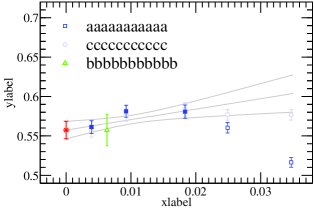
Figure 1: Extrapolation to the continuum limit of the decay constant ${F_{\rm D_{s}}}$. We also show the results of the recent simulation with non-perturbatively improved Wilson fermions in [2]. Only the data represented by filled squares entered the fit.

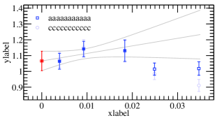
Figure 2: Extrapolation to the continuum limit of the ratio ${F_{\rm D_{s}^{\ast}}}/F_{\rm D_{s}}$. Only the data represented by filled squares entered the fit. Note that this quantity was extracted from data set A only, as the vector channel correlators are available only in this case.

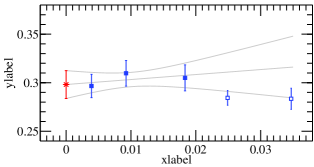
Figure 3: Extrapolation to the continuum limit of the mass splitting. Only the data represented by filled squares entered the fit. As in figure 2, this quantity was extracted from data set A only.

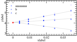
Figure 4: Extrapolation to the continuum limit of the RGI mass of the charm quark. Only the data represented by filled symbols entered the fit. For the red star and squares, the $c_{\rm A}$ of [20] (ALPHA) was used, while it is the one of [21] (LANL) for the grey data points.

4 Discussion

The approach of the data to the continuum limit for $r_{0}F_{\rm D_{s}}$, $F_{\rm D_{s}^{\ast}}/F_{\rm D_{s}}$, $r_{0}(m_{\rm D_{s}^{\ast}}-m_{\rm D_{s}})$ and the three definitions of the RGI charm quark mass is depicted in figures 1 – 4 for all five lattice spacings. As far as they enter, both sets of non-perturbative values for the improvement coefficient $c_{\rm A}(g_{0})$ of the axial-vector current, i.e. from ref. [20] (ALPHA) and from ref. [21] (LANL) and differing in the particular improvement conditions imposed for their determination, have been considered.

In ref. [35] a breakdown of ${\rm O}(a)$ improvement for improved Wilson quarks with heavy quark masses about $aM_{\rm h}\gtrsim 0.64$ was found in perturbation theory. Since the charm quark mass in lattice units is heavier than this bound for the two coarsest lattices with $a=0.093\,$fm and $a=0.079\,$fm, we exclude the results on these lattices from the continuum extrapolations. In fact, significant deviations from the linear dependence on $a^{2}$ of the data on the coarser lattices is observed for $r_{0}F_{\rm D_{s}}$ and $F_{\rm D_{s}^{\ast}}/F_{\rm D_{s}}$, and also for the charm quark mass definitions $r_{0}M_{\rm c}^{(\rm cs)}$ and $r_{0}M_{\rm c}^{(\rm cc)}$; in the latter case, however, only when using $c_{\rm A}$ by LANL. In general, on the coarsest two lattices we see significant discrepancies between the results of our non-perturbative computation obtained with the ALPHA-$c_{\rm A}$ and the LANL-$c_{\rm A}$, respectively, which is in line with perturbative criterion on $aM_{\rm h}$ consulted above.

For the final results in the continuum limit of quenched QCD we quote the linear extrapolation of the data at the three finest lattice spacings, where we employ the $c_{\rm A}$ of [20] for the improvement of the axial current. In this way we are well within the range of quark masses $aM_{\rm h}$, for which ${\rm O}(a)$ improvement and thus the validity of the $a^{2}$-expansion and the associated scaling behaviour are expected to hold. In addition, the ambiguity owing to the choice of $c_{\rm A}$ we observe has no significant effect at these lattice spacings. These data points are fully compatible with $(a\Lambda_{\rm QCD})^{2}$ corrections to the continuum limit when using $\Lambda_{\rm QCD}\approx 500$ MeV which also indicates that there are no large $(aM_{c})^{2}$-corrections.

The fact that the continuum limit of the three definitions of the RGI charm quark mass (12) – (14) yield compatible continuum extrapolated results demonstrates nicely the universality of the continuum limit and thereby provides strong evidence for the correctness of the extrapolation procedure. Our final results in units of the hadronic scale $r_{0}$ are collected in the bottom row of table 4. The quoted errors include all errors, i.e. the statistical ones, those stemming from the fits at intermediate stages of the analysis as well as the uncertainties of $r_{0}/a$ and the various $Z$-factors. Using $r_{0}=0.5\,$fm, we also convert our numbers to physical units: $F_{\rm D_{s}}=220(4)(?)\,$MeV, $m_{\rm D_{s}^{\ast}}-m_{\rm D_{s}}=118(6)(?)\,$MeV, $M_{\rm c}^{({\rm cs})}=1.59(2)(?)\,$GeV, $M_{\rm c}^{({\rm cc})}=1.60(2)(?)\,$GeV and $M_{\rm c}^{({\rm c})}=1.61(2)(?)\,$GeV. With the second error we indicate the unknown systematic contribution due to the quenched approximation, by which also the result for the dimensionless ratio $F_{\rm D_{s}^{\ast}}/F_{\rm D_{s}}$ is affected. Note that thanks to the additional, finer lattice spacing and the substantially increased total statistics in the pseudo-scalar channel, we have gained a factor of about two in accuracy for $r_{0}M_{\rm c}$ and $r_{0}F_{\rm D_{s}}$ compared to the earlier investigations of [14, 1].

Whereas in the case of the RGI charm quark mass we observe agreement within errors with the result of ref. [14], the continuum limit of $r_{0}F_{\rm D_{s}}$ quoted in [1], which is based on data set A for the range of lattice spacings $a\approx 0.08-0.05\,$fm, now proves to overestimate our result in table 4 for the leptonic decay constant of the ${\rm{D}_{s}}$-meson by about three standard deviations. We have identified two reasons for this: Firstly, after increasing the statistics for $r_{0}F_{\rm D_{s}}$ by generating data set B, the central value at $a=0.048\,$fm ($\beta=6.45$) moved down by about $1.5\sigma$. Secondly, in addition to [1] we now have results for a finer lattice spacing with $a=0.031\,$fm ($\beta=6.7859$). Thus, increasing the statistics by combining data set A and B, discarding the data point at $a=0.079\,$fm ($\beta=6.2$) from the continuum extrapolation and including the results at $a=0.031\,$fm instead causes a shift in the central value for $F_{\rm D_{s}}$ by about three standard deviations compared to the result in [1]. Statistical fluctuations in conjunction with leading plus possibly higher-order lattice artefacts can misguide the true continuum extrapolation.

This clearly reveals that it is indispensable to incorporate as small lattice spacings as possible into computations in the charm sector of ${\rm O}(a)$ improved lattice QCD, in order to get a controlled handle on the continuum limit.

5 Conclusion

Full QCD simulations with improved Wilson fermions in large volumes and at small lattice resolutions very close to the physical point are now feasible [36, 37]. Since their formulation is free of conceptual problems and since they are comparably cheap to simulate, they are now being applied on a large scale in the computation of Standard Model parameters at very high precision. The results of this work, although referring to the quenched approximation, emphasize the importance of performing a scaling study down to very small lattice spacings when calculating observables for hadrons containing a charm quark. Without the data at the finest lattice spacing and its satisfactory statistical accuracy obtained here, the continuum extrapolation would have yielded too large a value for $F_{\rm D_{s}}$ and also for $F_{\rm D_{s}^{\ast}}/F_{\rm D_{s}}$.

It is expected that these findings for the quenched theory carry over to the theory with dynamical sea quarks. We stress that only a scaling study of charmed observables down to extremely fine lattice spacings will allow for a reliable assessment of the cutoff effects. These findings, however, do not directly apply to other fermion discretizations and therefore, similar studies are crucial in each individual case.

- [1] ALPHA Collaboration, A. Jüttner and J. Rolf, A precise determination of the decay constant of the -meson in quenched QCD, Phys. Lett. B560 (2003) 59–63, [hep-lat/0302016].
- [2] A. Ali Khan et al., Decay constants of charm and beauty pseudoscalar heavy- light mesons on fine lattices, Phys. Lett. B652 (2007) 150–157, [hep-lat/0701015].
- [3] C. Aubin et al., Charmed meson decay constants in three-flavor lattice QCD, Phys. Rev. Lett. 95 (2005) 122002, [hep-lat/0506030].
- [4] HPQCD Collaboration, E. Follana, C. T. H. Davies, G. P. Lepage, and J. Shigemitsu, High Precision determination of the , , and decay constants from lattice QCD, Phys. Rev. Lett. 100 (2008) 062002, [arXiv:0706.1726].
- [5] B. Blossier, V. Lubicz, S. Simula, and C. Tarantino, Pseudoscalar meson decay constants , and from twisted mass Lattice QCD, arXiv:0810.3145.
- [6] ALPHA Collaboration, G. von Hippel, R. Sommer, J. Heitger, S. Schaefer, and N. Tantalo, physics from fine lattices, PoS LATTICE2008 (2008) 227, [arXiv:0810.0214].
- [7] J. L. Rosner and S. Stone, Decay Constants of Charged Pseudoscalar Mesons, 0802.1043.
- [8] CLEO Collaboration, M. Chadha et al., Improved measurement of the pseudoscalar decay constant , Phys. Rev. D58 (1998) 032002, [hep-ex/9712014].
- [9] CLEO Collaboration, K. M. Ecklund et al., Measurement of the absolute branching fraction of decay, Phys. Rev. Lett. 100 (2008) 161801, [arXiv:0712.1175].
- [10] CLEO Collaboration, M. Artuso et al., Measurement of the decay constant using , Phys. Rev. Lett. 99 (2007) 071802, [arXiv:0704.0629].
- [11] B. A. Dobrescu and A. S. Kronfeld, Accumulating evidence for nonstandard leptonic decays of mesons, Phys. Rev. Lett. 100 (2008) 241802, [arXiv:0803.0512].
- [12] M. Della Morte, Standard Model parameters and heavy quarks on the lattice, PoS LAT2007 (2007) 008, [arXiv:0711.3160].
- [13] A. Jüttner, Precision lattice computations in the heavy quark sector, Ph.D. thesis (2004) [hep-lat/0503040].
- [14] ALPHA Collaboration, J. Rolf and S. Sint, A precise determination of the charm quark’s mass in quenched QCD, JHEP 12 (2002) 007, [hep-ph/0209255].
- [15] M. Lüscher, R. Narayanan, P. Weisz, and U. Wolff, The Schrödinger Functional: A renormalizable probe for nonabelian gauge theories, Nucl. Phys. B384 (1992) 168–228, [hep-lat/9207009].
- [16] S. Sint, On the Schrödinger Functional in QCD, Nucl. Phys. B421 (1994) 135–158, [hep-lat/9312079].
- [17] M. Lüscher, S. Sint, R. Sommer, and P. Weisz, Chiral symmetry and improvement in lattice QCD, Nucl. Phys. B478 (1996) 365–400, [hep-lat/9605038].
- [18] ALPHA Collaboration, M. Guagnelli, J. Heitger, R. Sommer, and H. Wittig, Hadron masses and matrix elements from the QCD Schrödinger Functional, Nucl. Phys. B560 (1999) 465–481, [hep-lat/9903040].
- [19] M. Guagnelli and R. Sommer, Non-perturbative improvement of the vector current, Nucl. Phys. Proc. Suppl. 63 (1998) 886–888, [hep-lat/9709088].
- [20] M. Lüscher, S. Sint, R. Sommer, P. Weisz, and U. Wolff, Non-perturbative improvement of lattice QCD, Nucl. Phys. B491 (1997) 323–343, [hep-lat/9609035].
- [21] T. Bhattacharya, R. Gupta, W. Lee, and S. Sharpe, Scaling behavior of improvement and renormalization constants, Nucl. Phys. Proc. Suppl. 106 (2002) 789–791, [hep-lat/0111001].
- [22] J. Harada, S. Hashimoto, A. S. Kronfeld, and T. Onogi, Perturbative calculation of improvement coefficients, Phys. Rev. D67 (2003) 014503, [hep-lat/0208004].
- [23] M. Lüscher, S. Sint, R. Sommer, and H. Wittig, Non-perturbative determination of the axial current normalization constant in improved lattice QCD, Nucl. Phys. B491 (1997) 344–364, [hep-lat/9611015].
- [24] ALPHA Collaboration, M. Guagnelli et al., Non-perturbative results for the coefficients and in improved lattice QCD, Nucl. Phys. B595 (2001) 44–62, [hep-lat/0009021].
- [25] ALPHA Collaboration, S. Capitani, M. Lüscher, R. Sommer, and H. Wittig, Non-perturbative quark mass renormalization in quenched lattice QCD, Nucl. Phys. B544 (1999) 669–698, [hep-lat/9810063].
- [26] ALPHA Collaboration, M. Guagnelli, J. Heitger, F. Palombi, C. Pena, and A. Vladikas, The continuum limit of the quark mass step scaling function in quenched lattice QCD, JHEP 05 (2004) 001, [hep-lat/0402022].
- [27] S. Necco and R. Sommer, The heavy quark potential from short to intermediate distances, Nucl. Phys. B622 (2002) 328–346, [hep-lat/0108008].
- [28] Norddeutscher Verbund für Hoch- und Höchstleistungsrechnen, http://www.hlrn.de/.
- [29] The MILC code, http://www.physics.indiana.edu/~sg/milc.html.
- [30] ALPHA Collaboration, J. Garden, J. Heitger, R. Sommer, and H. Wittig, Precision computation of the strange quark’s mass in quenched QCD, Nucl. Phys. B571 (2000) 237–256, [hep-lat/9906013].
- [31] H. Leutwyler, The ratios of the light quark masses, Phys. Lett. B378 (1996) 313–318, [hep-ph/9602366].
- [32] ALPHA Collaboration, U. Wolff, Monte Carlo errors with less errors, Comput. Phys. Commun. 156 (2004) 143–153, [hep-lat/0306017].
- [33] Particle Data Group Collaboration, C. Amsler et al., Review of particle physics, Phys. Lett. B667 (2008) 1.
- [34] UKQCD Collaboration, K. C. Bowler et al., Decay constants of B and D mesons from non-perturbatively improved lattice QCD, Nucl. Phys. B619 (2001) 507–537, [hep-lat/0007020].
- [35] ALPHA Collaboration, M. Kurth and R. Sommer, Heavy quark effective theory at one-loop order: An explicit example, Nucl. Phys. B623 (2002) 271–286, [hep-lat/0108018].
- [36] L. Del Debbio, L. Giusti, M. Lüscher, R. Petronzio, and N. Tantalo, QCD with light Wilson quarks on fine lattices. I: First experiences and physics results, JHEP 02 (2007) 056, [hep-lat/0610059].
- [37] L. Del Debbio, L. Giusti, M. Lüscher, R. Petronzio, and N. Tantalo, QCD with light Wilson quarks on fine lattices. II: DD-HMC simulations and data analysis, JHEP 02 (2007) 082, [hep-lat/0701009].