Supersymmetry and other beyond the Standard Model physics: Prospects for determining mass, spin and CP properties

Abstract

The prospects of measuring masses, spin and CP properties within Supersymmetry and other beyond the Standard Model extensions at the LHC are reviewed. Emphasis is put on models with missing transverse energy due to undetected particles, as in Supersymmetry or Universal Extra Dimensions.

1 Introduction

It is widely expected that the Large Hadron Collider (LHC), which started very successfully on the 10th September 2008 with single beam injection, will uncover physics beyond the present Standard Model (SM) of particle physics. Supersymmetry (SUSY) is one of the most promising candidates for new physics. Among its virtues are the potential to overcome the hierarchy problem, to provide a dark matter candidate and make a unification of gauge coupling constants at a high energy scale possible. If the SUSY mass scale is in the sub-TeV range, already first LHC data will likely be sufficient to claim a discovery of new physics although new physics do not strictly mean SUSY as other new physics scenarios can have similar features and properties. In order to distinguish different scenarios of new physics and to determine the full set of model parameters within one scenario as many measurements of the new observed phenomena as possible are needed. This includes the precise measurement of masses, spins and CP properties of the newly observed particles.

Both multi-purpose experiments at the LHC, ATLAS [1] and CMS[2], are designed for these measurements. They will be able to pin down the exact model of new physics, e. g. to distinguish SUSY from Universal Extra Dimensions (UED).

2 Supersymmetry

In the following we assume R-parity conservation. As a consequence sparticles can only be produced in pairs and the lightest SUSY particle (LSP) is stable, which usually escapes detection in high-energy physics detectors. At LHC energies mostly pairs of squarks or gluinos are produced in proton-proton collisions, which then subsequently decay via long cascades into the LSP. Typical event topologies at the LHC are multi jet events with zero or more leptons and missing transverse energy due to the two LSPs. In the case of ATLAS these events will be triggered using a combined jet and missing $E_{T}$ trigger. The selection is mainly based on four jets ($p_{T}^{j_{1}}>100\,\mathrm{GeV}$, $p_{T}^{j_{2},j_{3},j_{4}}>50\,\mathrm{GeV}$) and missing $E_{T}$ ($E_{T}^{\mathrm{mis}}>100\,\mathrm{GeV},0.2m_{\mathrm{eff}}$). The effective mass, $m_{\mathrm{eff}}$, is the scalar sum of missing $E_{T}$ and the transverse momentum of the four leading jets. For further details see [3]. With this kind of selection minimal Supergravity (mSUGRA) models up to $m_{1/2}\sim 0.7\,\mathrm{TeV}$ or $m_{0}\sim 3\,\mathrm{TeV}$ can be discovered with a luminosity of 1 fb^-1.

2.1 Mass Measurements

Figure 1: Prime example of a SUSY decay chain for SUSY mass reconstruction. The first lepton in the decay chain is called the near lepton while the other is called the far lepton.

After the discovery of new physics beyond the SM as many measurements of the production process and particle properties are needed to pin-down the exact model of new physics. For example the masses of the new particles can be used to distinguish between different SUSY models. Due to the two escaping LSPs in every SUSY event, no mass peaks can be reconstructed and masses must be measured by other means. In mSUGRA models the main source of mass information is provided by ${{{\mathrm{{{}{}{{\widetilde{\chi}}_{{\mspace{1.0mu}{2}}}^{\mspace{1.0mu}{0}}}\mspace{-0.6mu}}}}}}$ decays, such as ${}{}{{}{{}{{{{{\mathrm{{{}{}{{\widetilde{\chi}}_{{\mspace{1.0mu}{2}}}^{\mspace{1.0mu}{0}}}\mspace{-0.6mu}}}}}}}}}}\to{}{}{{}{{}{{{{{{{}{}{{\widetilde{\ell}}_{\mspace{-2.0mu}{\mspace{0.0mu}}}^{\mspace{1.0mu}{{\raisebox{-0.06029pt}{{${{{\scriptstyle{{{{{{}}}}}}}}}$}}}}}}\mspace{-0.6mu}}}}}}}}}^{\pm}{}{{}{{{{{{{}{}{{\ell}_{\mspace{-2.0mu}{}}}\mspace{-0.6mu}}}}}}}}^{\mp}\to{}{}{{}{{}{{{{{\mathrm{{{}{}{{\widetilde{\chi}}_{{\mspace{1.0mu}{1}}}^{\mspace{1.0mu}{0}}}\mspace{-0.6mu}}}}}}}}}}{}{{}{{{{{{{}{}{{\ell}_{\mspace{-2.0mu}{}}}\mspace{-0.6mu}}}}}}}}^{+}{}{{}{{{{{{{}{}{{\ell}_{\mspace{-2.0mu}{}}}\mspace{-0.6mu}}}}}}}}^{-}$ (see Fig. 1). First we consider the invariant mass spectrum of the two leptons $m_{{}{{}{{{{{{{}{}{{\ell}_{\mspace{-2.0mu}{}}}\mspace{-0.6mu}}}}}}}}{}{{}{{{{{{{}{}{{\ell}_{\mspace{-2.0mu}{}}}\mspace{-0.6mu}}}}}}}}}$ from the decay chain in Fig. 1. Due to the scalar nature of the slepton, the invariant mass exhibits a triangular shape with a sharp drop-off at a maximal value $m_{{}{{}{{{{{{{}{}{{\ell}_{\mspace{-2.0mu}{}}}\mspace{-0.6mu}}}}}}}}{}{{}{{{{{{{}{}{{\ell}_{\mspace{-2.0mu}{}}}\mspace{-0.6mu}}}}}}}}}^{\mathrm{max}}$. The position of this endpoint depends on the masses of the involved sparticles:

$$m_{{}{{}{{{{{{{}{}{{\ell}_{\mspace{-2.0mu}{}}}\mspace{-0.6mu}}}}}}}}{}{{}{{{{{{{}{}{{\ell}_{\mspace{-2.0mu}{}}}\mspace{-0.6mu}}}}}}}}}^{\mathrm{max}}=m_{{}{}{{}{{}{{{{{\mathrm{{{}{}{{\widetilde{\chi}}_{{\mspace{1.0mu}{2}}}^{\mspace{1.0mu}{0}}}\mspace{-0.6mu}}}}}}}}}}}\sqrt{1-\left(\frac{m_{{}{}{{}{{}{{{{{{{}{}{{\widetilde{\ell}}_{\mspace{-2.0mu}{\mspace{0.0mu}}}^{\mspace{1.0mu}{{\raisebox{-0.04306pt}{{${{{\scriptstyle{{{{{{}}}}}}}}}$}}}}}}\mspace{-0.6mu}}}}}}}}}_{R}}}{m_{{}{}{{}{{}{{{{{\mathrm{{{}{}{{\widetilde{\chi}}_{{\mspace{1.0mu}{2}}}^{\mspace{1.0mu}{0}}}\mspace{-0.6mu}}}}}}}}}}}}\right)^{2}}\sqrt{1-\left(\frac{m_{{}{}{{}{{}{{{{{\mathrm{{{}{}{{\widetilde{\chi}}_{{\mspace{1.0mu}{1}}}^{\mspace{1.0mu}{0}}}\mspace{-0.6mu}}}}}}}}}}}}{m_{{}{}{{}{{}{{{{{{{}{}{{\widetilde{\ell}}_{\mspace{-2.0mu}{\mspace{0.0mu}}}^{\mspace{1.0mu}{{\raisebox{-0.04306pt}{{${{{\scriptstyle{{{{{{}}}}}}}}}$}}}}}}\mspace{-0.6mu}}}}}}}}}_{R}}}\right)^{2}}.$$ (1)

Combinatorial background from SM and other SUSY processes is subtracted using the flavor-subtraction method. The endpoint is measured from the di-lepton (electron and muon) mass distribution $N({}{{}{{{{{\mathrm{{{}{}{{e}^{-}}\mspace{-0.6mu}}}}}}}}}{}{{}{{{{{\mathrm{{{}{}{{e}^{+}}\mspace{-0.6mu}}}}}}}}})/\beta+\beta N({}{{}{{{{{\mathrm{{{}{}{{\mu}^{-}}\mspace{-0.6mu}}}}}}}}}{}{{}{{{{{\mathrm{{{}{}{{\mu}^{+}}\mspace{-0.6mu}}}}}}}}})-N({}{{}{{{{{\mathrm{{{}{}{{e}^{\pm}}\mspace{-0.6mu}}}}}}}}}{}{{}{{{{{\mathrm{{{}{}{{\mu}^{\mp}}\mspace{-0.6mu}}}}}}}}})$, where $N$ is the number of selected events and $\beta$ is the ratio of the electron and muon reconstruction efficiency ($\beta\simeq 0.86$) [3]. Figure 2 shows the mass distribution for different mSUGRA benchmark points. The SU3 point is an example of a simple two-body decay (Fig. 2(b)), SU4 illustrates a more complex three-body decay (Fig. 2(c)) and SU1 two two-body decays (Fig. 2(a)). In all cases the $m_{{}{{}{{{{{{{}{}{{\ell}_{\mspace{-2.0mu}{}}}\mspace{-0.6mu}}}}}}}}{}{{}{{{{{{{}{}{{\ell}_{\mspace{-2.0mu}{}}}\mspace{-0.6mu}}}}}}}}}$ endpoint can be measured without a bias although the needed luminosity is quite different. Further, the fit function to extract the endpoint(s) needs to be adjusted to the underlying mass spectrum. The expected sensitivity is summarized in Tab. 1 including the assumed luminosity.

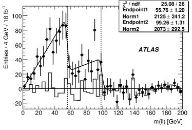
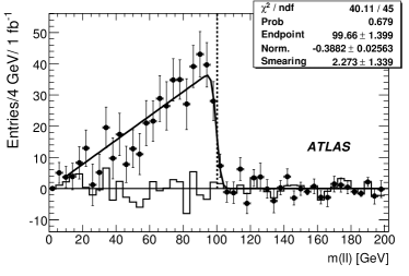
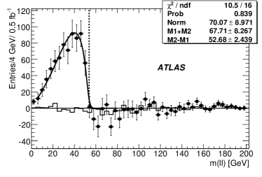
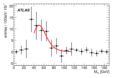
Figure 2: Flavour subtracted di-lepton mass spectrum for different mSUGRA benchmark points: (a) SU1(${}{{}{{{{{{{}{}{{\ell}_{\mspace{-2.0mu}{}}}\mspace{-0.6mu}}}}}}}}=e,{}{{}{{{{{\mathrm{{{}{}{{\mu}}\mspace{-0.6mu}}}}}}}}}$), (b) SU3(${}{{}{{{{{{{}{}{{\ell}_{\mspace{-2.0mu}{}}}\mspace{-0.6mu}}}}}}}}=e,{}{{}{{{{{\mathrm{{{}{}{{\mu}}\mspace{-0.6mu}}}}}}}}}$), (c) SU4(${}{{}{{{{{{{}{}{{\ell}_{\mspace{-2.0mu}{}}}\mspace{-0.6mu}}}}}}}}=e,{}{{}{{{{{\mathrm{{{}{}{{\mu}}\mspace{-0.6mu}}}}}}}}}$), (d) SU3(${}{{}{{{{{{{}{}{{\ell}_{\mspace{-2.0mu}{}}}\mspace{-0.6mu}}}}}}}}={}{{}{{{{{\mathrm{{{}{}{{\tau}}\mspace{-0.6mu}}}}}}}}}$).

observable	benchmark point	true mass [GeV]	expected mass [GeV]	luminosity [fb-1]
$m_{{}{{}{{{{{{{}{}{{\ell}_{\mspace{-2.0mu}{}}}\mspace{-0.6mu}}}}}}}}{}{{}{{{{{{{}{}{{\ell}_{\mspace{-2.0mu}{}}}\mspace{-0.6mu}}}}}}}}}$	SU1	56.1	$55.8\pm 1.2\pm 0.2$	18
$m_{{}{{}{{{{{{{}{}{{\ell}_{\mspace{-2.0mu}{}}}\mspace{-0.6mu}}}}}}}}{}{{}{{{{{{{}{}{{\ell}_{\mspace{-2.0mu}{}}}\mspace{-0.6mu}}}}}}}}}$	SU1	97.9	$99.3\pm 1.3\pm 0.3$	18
$m_{{}{{}{{{{{{{}{}{{\ell}_{\mspace{-2.0mu}{}}}\mspace{-0.6mu}}}}}}}}{}{{}{{{{{{{}{}{{\ell}_{\mspace{-2.0mu}{}}}\mspace{-0.6mu}}}}}}}}}$	SU3	100.2	$99.7\pm 1.4\pm 0.3$	1.0
$m_{{}{{}{{{{{\mathrm{{{}{}{{\tau}}\mspace{-0.6mu}}}}}}}}}{}{{}{{{{{\mathrm{{{}{}{{\tau}}\mspace{-0.6mu}}}}}}}}}}$	SU3	98	$102\pm 17\pm 5.5\pm 7$	1.0
$m_{{}{{}{{{{{{{}{}{{\ell}_{\mspace{-2.0mu}{}}}\mspace{-0.6mu}}}}}}}}{}{{}{{{{{{{}{}{{\ell}_{\mspace{-2.0mu}{}}}\mspace{-0.6mu}}}}}}}}}$	SU4	53.6	$52.7\pm 2.4\pm 0.2$	0.5
$m_{{}{{}{{{{{{{}{}{{q}_{\mspace{-2.0mu}{}}}\mspace{-0.6mu}}}}}}}}{}{{}{{{{{{{}{}{{\ell}_{\mspace{-2.0mu}{}}}\mspace{-0.6mu}}}}}}}}\mathrm{(low)}}^{\mathrm{max}}$	SU3	325	$333\pm 6\pm 6\pm 8$	1.0
$m_{{}{{}{{{{{{{}{}{{q}_{\mspace{-2.0mu}{}}}\mspace{-0.6mu}}}}}}}}{}{{}{{{{{{{}{}{{\ell}_{\mspace{-2.0mu}{}}}\mspace{-0.6mu}}}}}}}}\mathrm{(high)}}^{\mathrm{max}}$	SU3	418	$445\pm 11\pm 11\pm 11$	1.0
$m_{{}{{}{{{{{{{}{}{{q}_{\mspace{-2.0mu}{}}}\mspace{-0.6mu}}}}}}}}{}{{}{{{{{{{}{}{{\ell}_{\mspace{-2.0mu}{}}}\mspace{-0.6mu}}}}}}}}{}{{}{{{{{{{}{}{{\ell}_{\mspace{-2.0mu}{}}}\mspace{-0.6mu}}}}}}}}}^{\mathrm{min}}$	SU3	249	$265\pm 17\pm 15\pm 7$	1.0
$m_{{}{{}{{{{{{{}{}{{q}_{\mspace{-2.0mu}{}}}\mspace{-0.6mu}}}}}}}}{}{{}{{{{{{{}{}{{\ell}_{\mspace{-2.0mu}{}}}\mspace{-0.6mu}}}}}}}}{}{{}{{{{{{{}{}{{\ell}_{\mspace{-2.0mu}{}}}\mspace{-0.6mu}}}}}}}}}^{\mathrm{max}}$	SU3	501	$501\pm 30\pm 10\pm 13$	1.0

Table 1: Reconstructed endpoint positions. The first error of the expected value is the statistical error and the second is due to systematic from the lepton energy scale and $\beta$. In case of $m_{{}{{}{{{{{\mathrm{{{}{}{{\tau}}\mspace{-0.6mu}}}}}}}}}{}{{}{{{{{\mathrm{{{}{}{{\tau}}\mspace{-0.6mu}}}}}}}}}}$ the third error is due to the uncertainty in the tau polarization.

A similar analysis can be performed if we replaced electrons and muons by taus. Due to the additional neutrinos from the tau decay, the visible di-tau mass distribution is not triangular any more (see Fig. 2(d)). This complicates measuring the endpoint of the spectrum. A solution to this problem is to fit a suitable function to the trailing edge of the visible di-tau mass spectrum and use the inflection point as an endpoint sensitive observable, which can be related to the true endpoint using a simple MC based calibration procedure. Figure 2(d) shows the charge subtracted visible di-tau mass distribution $N({}{{}{{{{{\mathrm{{{}{}{{\tau}^{-}}\mspace{-0.6mu}}}}}}}}}{}{{}{{{{{\mathrm{{{}{}{{\tau}^{+}}\mspace{-0.6mu}}}}}}}}})-N({}{{}{{{{{\mathrm{{{}{}{{\tau}^{\pm}}\mspace{-0.6mu}}}}}}}}}{}{{}{{{{{\mathrm{{{}{}{{\tau}^{\pm}}\mspace{-0.6mu}}}}}}}}})$ which is used to suppress background from fake taus and combinatorial background. The expected sensitivity is listed in Tab. 1. Please note, that the third error is due to the SUSY-model dependent polarization of the two taus. On the other hand this influence of the tau polarization on the di-tau mass distribution can be used to measure the tau polarization from the mass distribution and distinguish different SUSY models from each other.

By including the jet produced in association with the ${{{\mathrm{{{}{}{{\widetilde{\chi}}_{{\mspace{1.0mu}{2}}}^{\mspace{1.0mu}{0}}}\mspace{-0.6mu}}}}}}$ in the ${}{}{{}{{}{{{{{{{}{}{{\widetilde{q}}_{\mspace{-2.0mu}{\mspace{0.0mu}}}^{\mspace{1.0mu}{{\raisebox{-0.06029pt}{{${{{\scriptstyle{{{{{{}}}}}}}}}$}}}}}}\mspace{-0.6mu}}}}}}}}}_{L}$ decay (see Fig. 1), several other endpoints of measurable mass combinations are possible: $m_{{}{{}{{{{{{{}{}{{q}_{\mspace{-2.0mu}{}}}\mspace{-0.6mu}}}}}}}}{}{{}{{{{{{{}{}{{\ell}_{\mspace{-2.0mu}{}}}\mspace{-0.6mu}}}}}}}}\mathrm{(low)}}^{\mathrm{max}}$, $m_{{}{{}{{{{{{{}{}{{q}_{\mspace{-2.0mu}{}}}\mspace{-0.6mu}}}}}}}}{}{{}{{{{{{{}{}{{\ell}_{\mspace{-2.0mu}{}}}\mspace{-0.6mu}}}}}}}}\mathrm{(high)}}^{\mathrm{max}}$, $m_{{}{{}{{{{{{{}{}{{q}_{\mspace{-2.0mu}{}}}\mspace{-0.6mu}}}}}}}}{}{{}{{{{{{{}{}{{\ell}_{\mspace{-2.0mu}{}}}\mspace{-0.6mu}}}}}}}}{}{{}{{{{{{{}{}{{\ell}_{\mspace{-2.0mu}{}}}\mspace{-0.6mu}}}}}}}}}^{\mathrm{min}}$, $m_{{}{{}{{{{{{{}{}{{q}_{\mspace{-2.0mu}{}}}\mspace{-0.6mu}}}}}}}}{}{{}{{{{{{{}{}{{\ell}_{\mspace{-2.0mu}{}}}\mspace{-0.6mu}}}}}}}}{}{{}{{{{{{{}{}{{\ell}_{\mspace{-2.0mu}{}}}\mspace{-0.6mu}}}}}}}}}^{\mathrm{max}}$. The label min/max denotes the upper/lower endpoint of the spectrum. In the case of $m_{{}{{}{{{{{{{}{}{{q}_{\mspace{-2.0mu}{}}}\mspace{-0.6mu}}}}}}}}{}{{}{{{{{{{}{}{{\ell}_{\mspace{-2.0mu}{}}}\mspace{-0.6mu}}}}}}}}\mathrm{}}^{\mathrm{max}}$ the near and the far lepton can not be distinguished in most of the SUSY models and instead the minimum/maximum of the mass $m_{{}{{}{{{{{{{}{}{{q}_{\mspace{-2.0mu}{}}}\mspace{-0.6mu}}}}}}}}{}{{}{{{{{{{}{}{{\ell}_{\mspace{-2.0mu}{}}^{\pm}}\mspace{-0.6mu}}}}}}}}}$ is used. As in the di-lepton case a suitable fit function for each observable is needed. The expected sensitivity to the different mass combinations for the SU3 model are summarized in Tab. 1.

These five mass combinations can be used to extract the underlying high mass model parameters using fitting programs like Fittino[4] or SFitter[5].

2.2 Spin Measurements

Measuring the number of new particles and their masses will give us enough information to extract model parameters for a certain extension of the SM. However, the mass information will not always be enough to distinguish different scenarios of new physics. For example, UED with Kaluza-Klein (KK) parity can be tuned in such a way that it reproduces the mass spectrum of certain SUSY models. However, the spin of the new particles is different and can be used to discriminate between these models.

The standard SUSY decay chain (see Fig. 1) can also be used to measure the spin of ${{{\mathrm{{{}{}{{\widetilde{\chi}}_{{\mspace{1.0mu}{2}}}^{\mspace{1.0mu}{0}}}\mspace{-0.6mu}}}}}}$ [6]. A charge asymmetry $A$ is expected in the invariant masses $m_{{}{{}{{{{{{{}{}{{q}_{\mspace{-2.0mu}{}}}\mspace{-0.6mu}}}}}}}}{}{{}{{{{{{{}{}{{\ell}_{\mspace{-2.0mu}{}}}\mspace{-0.6mu}}}}}}}}^{\mathrm{near(\pm)}}}$ formed by the quark and the near lepton. It is defined as $A=(s^{+}-s^{-})/(s^{+}+s^{-})$, where $s^{\pm}=d\sigma/dm_{{}{{}{{{{{{{}{}{{q}_{\mspace{-2.0mu}{}}}\mspace{-0.6mu}}}}}}}}{}{{}{{{{{{{}{}{{\ell}_{\mspace{-2.0mu}{}}}\mspace{-0.6mu}}}}}}}}^{\mathrm{near(\pm)}}}$. In most of the cases it is experimentally not possible to distinguish between near and far lepton and hence only $m_{{}{{}{{{{{{{}{}{{q}_{\mspace{-2.0mu}{}}}\mspace{-0.6mu}}}}}}}}{}{{}{{{{{{{}{}{{\ell}_{\mspace{-2.0mu}{}}}\mspace{-0.6mu}}}}}}}}^{\mathrm{\pm}}}$ can be measured, diluting $A$. Further, the asymmetry from the corresponding $m_{{}{}{{}{{}{{{{{{{}{}{{\overline{q}}_{\mspace{-2.0mu}{\mspace{1.0mu}{}}}^{\mspace{1.0mu}{{\raisebox{-1.18402pt}{{${{{\scriptstyle{{{{{{}}}}}}}}}$}}}}}}\mspace{-0.6mu}}}}}}}}}{}{{}{{{{{{{}{}{{\ell}_{\mspace{-2.0mu}{}}^{\mp}}\mspace{-0.6mu}}}}}}}}}$ charge distribution is the same as the asymmetry for $m_{{}{{}{{{{{{{}{}{{q}_{\mspace{-2.0mu}{}}}\mspace{-0.6mu}}}}}}}}{}{{}{{{{{{{}{}{{\ell}_{\mspace{-2.0mu}{}}}\mspace{-0.6mu}}}}}}}}^{\mathrm{\pm}}}$, but with opposite sign. Usually it is not possible to distinguish ${{{{}{}{{q}_{\mspace{-2.0mu}{}}}\mspace{-0.6mu}}}}$ jets from ${{{{}{}{{\overline{q}}_{\mspace{-2.0mu}{\mspace{1.0mu}{}}}^{\mspace{1.0mu}{{\raisebox{-1.65764pt}{{${{{\scriptstyle{{{{{{}}}}}}}}}$}}}}}}\mspace{-0.6mu}}}}$ jets at the LHC. On the other side more squarks than anti-squarks will be produced. The expected asymmetry $A$ for SU3 is shown in Fig. 4 for a luminosity of 30 fb^-1, where already 10 fb^-1 are sufficient to exclude the zero spin hypothesis at 99% CL[7]. In the case of SU1 far and near leptons are distinguishable on kinematic grounds. On the other hand, cross section times branching ratio of this decay chain is much lower than the SU3 case, so that 100 fb^-1 are needed to exclude the zero spin hypothesis at 99% CL.

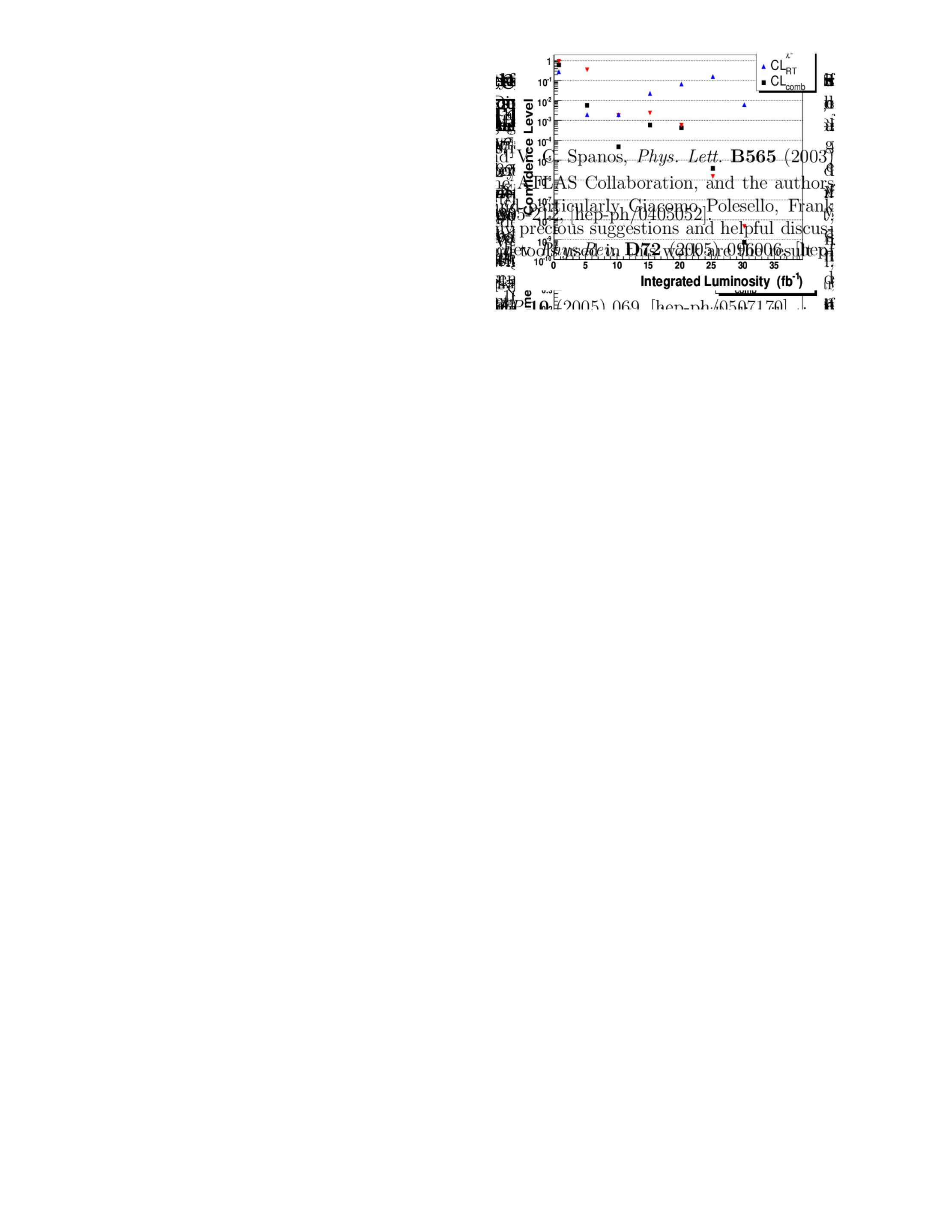
Figure 3: Expected charge asymmetry $A$ for SU3 and 30 fb^-1.

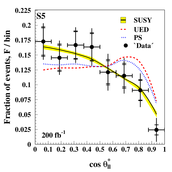
Figure 4: Expected $\theta^{*}_{ll}$ distribution for the S5 bench mark point and 200 fb^-1.

The slepton spin can be measured in direct di-slepton production ${}{{}{{{{{{{}{}{{q}_{\mspace{-2.0mu}{}}}\mspace{-0.6mu}}}}}}}}{}{}{{}{{}{{{{{{{}{}{{\overline{q}}_{\mspace{-2.0mu}{\mspace{1.0mu}{}}}^{\mspace{1.0mu}{{\raisebox{-1.65764pt}{{${{{\scriptstyle{{{{{{}}}}}}}}}$}}}}}}\mspace{-0.6mu}}}}}}}}}\to{}{{}{{{{{\mathrm{{{}{}{{Z}}\mspace{-0.6mu}}}}}}}}}{}{{}{{{{{\mathrm{{{}{}{{\gamma}}\mspace{-0.6mu}}}}}}}}}\to{}{}{{}{{}{{{{{{{}{}{{\widetilde{\ell}}_{\mspace{-2.0mu}{\mspace{0.0mu}}}^{\mspace{1.0mu}{{\raisebox{-0.06029pt}{{${{{\scriptstyle{{{{{{}}}}}}}}}$}}}}}}\mspace{-0.6mu}}}}}}}}}{}{}{{}{{}{{{{{{{}{}{{\widetilde{\ell}}_{\mspace{-2.0mu}{\mspace{0.0mu}}}^{\mspace{1.0mu}{{\raisebox{-0.06029pt}{{${{{\scriptstyle{{{{{{}}}}}}}}}$}}}}}}\mspace{-0.6mu}}}}}}}}}\to{}{}{{}{{}{{{{{\mathrm{{{}{}{{\widetilde{\chi}}_{{\mspace{1.0mu}{}}}^{\mspace{1.0mu}{0}}}\mspace{-0.6mu}}}}}}}}}}{}{{}{{{{{{{}{}{{\ell}_{\mspace{-2.0mu}{}}}\mspace{-0.6mu}}}}}}}}{}{}{{}{{}{{{{{\mathrm{{{}{}{{\widetilde{\chi}}_{{\mspace{1.0mu}{}}}^{\mspace{1.0mu}{0}}}\mspace{-0.6mu}}}}}}}}}}{}{{}{{{{{{{}{}{{\ell}_{\mspace{-2.0mu}{}}}\mspace{-0.6mu}}}}}}}}$. In UED the corresponding process is ${}{{}{{{{{{{}{}{{q}_{\mspace{-2.0mu}{}}}\mspace{-0.6mu}}}}}}}}{}{}{{}{{}{{{{{{{}{}{{\overline{q}}_{\mspace{-2.0mu}{\mspace{1.0mu}{}}}^{\mspace{1.0mu}{{\raisebox{-1.65764pt}{{${{{\scriptstyle{{{{{{}}}}}}}}}$}}}}}}\mspace{-0.6mu}}}}}}}}}\to{}{{}{{{{{\mathrm{{{}{}{{Z}}\mspace{-0.6mu}}}}}}}}}{}{{}{{{{{\mathrm{{{}{}{{\gamma}}\mspace{-0.6mu}}}}}}}}}\to{}{{}{{{{{{{}{}{{\ell}_{\mspace{-2.0mu}{}}}\mspace{-0.6mu}}}}}}}}_{1}{}{{}{{{{{{{}{}{{\ell}_{\mspace{-2.0mu}{}}}\mspace{-0.6mu}}}}}}}}_{1}\to{}{{}{{{{{\mathrm{{{}{}{{\gamma}}\mspace{-0.6mu}}}}}}}}}_{1}{}{{}{{{{{{{}{}{{\ell}_{\mspace{-2.0mu}{}}}\mspace{-0.6mu}}}}}}}}{}{{}{{{{{\mathrm{{{}{}{{\gamma}}\mspace{-0.6mu}}}}}}}}}_{1}{}{{}{{{{{{{}{}{{\ell}_{\mspace{-2.0mu}{}}}\mspace{-0.6mu}}}}}}}}$, where ${}{{}{{{{{{{}{}{{\ell}_{\mspace{-2.0mu}{}}}\mspace{-0.6mu}}}}}}}}_{1}$ and ${}{{}{{{{{\mathrm{{{}{}{{\gamma}}\mspace{-0.6mu}}}}}}}}}_{1}$ are the KK-lepton and -photon, respectively. Both have spin $1/2$, the same as their SM partners. In both decay chains a SM lepton-pair is produced, all other particles escape undetected. Although the involved new particle masses can be the same, the slepton spin ($0$) and KK-lepton spin ($1/2$) are different. The angle $\theta^{*}$, as defined between the incoming quark and the slepton/KK-lepton, can be used to discriminate between both model. The pure phase space (PS) distribution would be flat. In SUSY and UED models it is proportional to $1+A\cos^{2}\theta^{*}$, where $A=-1$ for SUSY and $A=(E^{2}_{{}{{}{{{{{{{}{}{{\ell}_{\mspace{-2.0mu}{}}}\mspace{-0.6mu}}}}}}}}_{1}}-m^{2}_{{}{{}{{{{{{{}{}{{\ell}_{\mspace{-2.0mu}{}}}\mspace{-0.6mu}}}}}}}}_{1}})/(E^{2}_{{}{{}{{{{{{{}{}{{\ell}_{\mspace{-2.0mu}{}}}\mspace{-0.6mu}}}}}}}}_{1}}+m^{2}_{{}{{}{{{{{{{}{}{{\ell}_{\mspace{-2.0mu}{}}}\mspace{-0.6mu}}}}}}}}_{1}})$ for UED. However, $\theta^{*}$ is not directly accessible. Experimentally only $\theta^{*}_{ll}\equiv\cos\left(2\tan^{-1}\exp\left(\Delta\eta_{{}{{}{{{{{{{}{}{{\ell}_{\mspace{-2.0mu}{}}^{+}}\mspace{-0.6mu}}}}}}}}{}{{}{{{{{{{}{}{{\ell}_{\mspace{-2.0mu}{}}^{-}}\mspace{-0.6mu}}}}}}}}}/2\right)\right)=\tanh\left(\Delta\eta_{{}{{}{{{{{{{}{}{{\ell}_{\mspace{-2.0mu}{}}^{+}}\mspace{-0.6mu}}}}}}}}{}{{}{{{{{{{}{}{{\ell}_{\mspace{-2.0mu}{}}^{-}}\mspace{-0.6mu}}}}}}}}}/2\right)$, the angle between the two leptons, can be measured. Note, that $\theta^{*}_{ll}$ is invariant under boosts along the beam axis. Still, $\theta^{*}_{ll}$ has some correlation with $\theta^{*}$. Events with two good leptons ($p_{T}^{l_{1},l_{2}}>40,30\,\mathrm{GeV}$) and missing $E_{T}>100\,\mathrm{GeV}$ are selected. Further, events with b-jets and high $p_{T}$ jets ($p_{T}>100\,\mathrm{GeV}$) are rejected[8]. The expected $\theta^{*}_{ll}$ distribution for a luminosity of 200 fb^-1 is shown in Fig. 4 including the predictions for the SUSY, UED and PS case. Clearly, the difference between all three cases can be see. For a five sigma significance 200 fb^-1 are needed to distinguish between SUSY and UED and 350 fb^-1 to distinguish between SUSY and PS.

3 Other Beyond the Standard Model Physics

The previous section was devoted to the measurement of masses and spins in the case of missing energy due to non detectable new particles within cascade decays. Without this complication the measurement of masses and spins of new particles is straight forward. As an example we will discuss the graviton case[9]. The graviton, which should be a spin 2 particle, can be produced directly in proton-proton collisions at the LHC. The decay channel $G\to{}{{}{{{{{\mathrm{{{}{}{{e}^{-}}\mspace{-0.6mu}}}}}}}}}{}{{}{{{{{\mathrm{{{}{}{{e}^{+}}\mspace{-0.6mu}}}}}}}}}$ can be cleanly selected. The mass of the graviton resonance can be directly measured from the di-electron invariant mass distribution. For a given luminosity of 100 fb^-1 the graviton with $m_{G}$ up to 2080 GeV can be discovered. $\theta^{*}$, the angle between the electron and the beam axis, can be used to measure the spin of the observed resonance. The general form of the $\cos\theta^{*}$ distribution is $1+A\cos^{2}\theta^{*}+B\cos^{4}\theta^{*}$. For graviton production via gluons or quarks the factors are $A=0,B=-1$ and $A=-3,B=4$, respectively. Further, the SM background is only flat ($A=0,B=0$) for electron-pair production via a scalar resonance. In the case of a vector resonance $A=\alpha,B=0$, where $\alpha=1$ in the SM. For a given luminosity of 100 fb^-1 the spin 2 nature of the graviton can be determined at 90% CL up to graviton masses of 1720 GeV, which also means that the spin 1 case is ruled out.

4 Summary

Provided new particles are in the sub-TeV regime, already first LHC data will allow to perform a rough spectroscopy of these. In the case of no missing energy due to invisible particles at the end of a decay chain, the experimental methods for mass and spin measurements are very well established and can be applied at the LHC. In the case of missing energy the experimental methods to measure mass and spin of the new particles are quite advanced and will be needed to distinguish for example SUSY from UED. Clearly, some of the more difficult measurements need high luminosity.

1

References

• [1] ATLAS Collaboration, G. Aad et al., JINST 3, S08003 (2008)
• [2] CMS Collaboration, R. Adolphi et al., JINST 3, S08004 (2008)
• [3] ATLAS Collaboration, Expected Performance of the ATLAS Experiment, Detector, Trigger and Physics. CERN-OPEN-2008-020, Geneva, 2008, to appear
• [4] P. Bechtle, K. Desch, and P. Wienemann, Comput. Phys. Commun. 174, 47 (2006). hep-ph/0412012
• [5] R. Lafaye, T. Plehn, M. Rauch, and D. Zerwas, Eur. Phys. J. C54, 617 (2008). 0709.3985
• [6] A. J. Barr, Phys. Lett. B596, 205 (2004). hep-ph/0405052
• [7] M. Biglietti et al. ATL-PHYS-PUB-2007-004
• [8] A. J. Barr, JHEP 02, 042 (2006). hep-ph/0511115
• [9] B. C. Allanach, K. Odagiri, M. A. Parker, and B. R. Webber, JHEP 09, 019 (2000). hep-ph/0006114