Oscillations of the Inner Regions of Viscous Accretion Disks

Abstract

Although quasi-periodic oscillations (QPOs) have been discovered in different X-ray sources, their origin is still a matter of debate. Analytical studies of hydrodynamic accretion disks have shown three types of trapped global modes with properties that appear to agree with the observations. However, these studies take only linear effects into account and do not address the issues of mode excitation and decay. Moreover, observations suggest that resonances between modes play a crucial role. A systematic, numerical study of this problem is therefore needed. In this paper, we use a pseudo-spectral algorithm to perform a parameter study of the inner regions of hydrodynamic disks. By assuming $\alpha$-viscosity, we show that steady state solutions rarely exist. The inner edges of the disks oscillate and excite axisymmetric waves. In addition, the flows inside the inner edges are sometimes unstable to non-axisymmetric perturbations. One-armed, or even two-armed, spirals are developed, which provides a plausible explanation for the high-frequency QPOs observed from accreting black holes. When the Reynolds numbers are above certain critical values, the inner disks go through some transient turbulent states characterized by strong trailing spirals; while large-scale leading spirals developed in the outer disks. We compared our numerical results with standard thin disk oscillation models. Although the non-axisymmetric features have their analytical counterparts, more careful study is needed to explain the axisymmetric oscillations.

1. Introduction

Quasi-periodic oscillations (QPOs) are strong coherent features in the power density spectra (PDS) that are found in different low mass X-ray binaries (LMXBs, see the review article by van der Klis 2006 and Remillard & McClintock 2006). Their frequencies range from $\sim 300$ to $\sim 1200$ Hz, suggesting that they correspond to accretion flows very close to the central objects (van der Klis, 2000, 2006). Understanding the origin of QPOs will, therefore, lead to precise measurements of black hole spins as well as direct tests of Einstein’s equivalent principle (Psaltis 2004, but also see Psaltis et al. 2008). Although several models have been proposed in the last decade to explain some aspects of the observations, the origin of QPOs is still a matter of debate.

Local analytical studies of hydrodynamic accretion disks have shown three types of trapped global modes (see the review article by Kato 2001, hereafter K01, and references therein, or more recently Wagoner 2008). The coupling between inertial oscillations and pressure variations lead to two different frequencies. The higher frequencies correspond to inertial acoustic $p$-modes and the lower ones correspond to gravity $g$-modes (Perez et al., 1997; Ortega-Rodríguez et al., 2002). Oscillations in the vertical direction are called corrugation $c$-modes (Silbergleit et al., 2001). Although these oscillations have properties that appear to agree with the observations, analytical studies can take only the linear effects into account and they do not address issues of mode excitation, propagation, and decay. Moreover, observations of QPOs in black holes strongly suggest that resonances between modes play a crucial role (Abramowicz & Kluźniak, 2001; Kluzniak & Abramowicz, 2001). This fact has led to the development of non-linear models (for example, Kato, 2004, 2008a, 2008b).

In principle, numerical simulations can be used to test these models, including both linear and non-linear ones. One would like to carry out simulations for many dynamical time scales to obtain accurate PDS and study their temporal variability. However, even with the Shakura & Syunyaev (1973) $\alpha$-viscosity (which greatly simplifies the problem) the effective/turbulent Reynolds numbers in thin accretion disks are still beyond the value that one could perform direct numerical simulations with standard numerical methods.

We have developed earlier a two-dimensional, pseudo-spectral algorithm in order to model thin accretion flows around black holes (Chan et al., 2005). Spectral methods are high-order numerical methods that have a very small numerical dissipation. For two-dimensional flows, they are at least an order of magnitude more efficient then (low order) finite difference methods. Our algorithm solves the hydrodynamic equations in the disk plane (i.e., with $r$ and $\phi$) by using the thin disk approximation. In addition to the $\alpha$-viscosity, high-order artificial viscosity is implemented by using a spectral filter, which affects only the large wavenumber modes and preserves correct shock properties (see Ma, 1998a, b, for details). We use a buffer zone to absorb outgoing waves at the outer boundary. For the inner boundary, because the flow is always super-sonic (toward the central object), no explicit boundary condition is needed. We apply this algorithm to study the very inner regions of two-dimensional, viscous, polytropic accretion disks around a black hole with zero spin.

We find that steady state solutions do not exist for most combinations of the parameters. The inner edges of the disk often oscillate and excite axisymmetric waves with propagates all the way to the outer boundary. Other than that, non-axisymmetric spirals are sometimes developed in the simulations and provide a plausible explanation of the QPOs. Depending on the values of the parameters, these spirals can be classified as inner one-armed spirals or inner two-armed spirals; in the cases with extreme Reynolds numbers, the results are steady global one-armed spirals. Although detailed study of all these features is beyond the scope of this paper, we will make connections between the observed numerical phenomena and the standard analytical models.

This paper is organized as following. The assumptions and the governing equations of the problem are presented in the next section. In §3, we derive an approximate steady state solution, which is used to initialize our simulations. We summarize the results from our simulations in §4 and describe our temporal analysis method in §5. Detailed discussions of different important features are presented in the subsequent sections, namely, the axisymmetric rings in §6, non-axisymmetric spirals in §7, and the steady global spirals in §8. We describe the limitations of our study in §9. Finally, we conclude with a discussion and suggest future research direction in §10.

2. Assumptions and Equations

We are interested in the dynamics of thin accretion disks. For simplicity, we neglect the motion in the vertical direction. By assuming a polytropic equation of state, the hydrodynamics is fully described by only three quantities, namely, the column density $\Sigma$ and the two velocity components in the disk plane $v_{r}$, $v_{\phi}$. The governing equations are thus given by the continuity equation

$$\frac{\partial\Sigma}{\partial t}+\nabla\cdot(\Sigma\mathbf{v})=0$$ (1)

and the (two-dimensional) Navier-Stokes equation

$$\Sigma\frac{\partial\mathbf{v}}{\partial t}+\Sigma(\mathbf{v}\cdot\nabla)\mathbf{v}=-\nabla P+\nabla\mathbf{\tau}+\Sigma\;\mathbf{g}.$$ (2)

In the above equations, $P=K\Sigma^{\Gamma}$ is the height-integrated thermal pressure with $K$ and $\Gamma$ being the polytropic constant and polytropic index. We denote by $\tau$ the viscosity tensor, which (in Cartesian coordinates) is given by

$$\tau_{i\!j}=\nu_{\mathrm{SS}}\Sigma\left[\left(\frac{\partial v_{i}}{\partial x_{j}}+\frac{\partial v_{j}}{\partial x_{i}}\right)-\frac{2}{3}(\nabla\cdot\mathbf{v})\;\delta_{ij}\right].$$ (3)

We also define the sound speed $c_{\mathrm{s}}\equiv(\Gamma P/\Sigma)^{1/2}$ and the scale height $H\equiv c_{\mathrm{s}}/\Omega_{\mathrm{K}}$, where $\Omega_{\mathrm{K}}$ is the “Keplerian” frequency defined below.

We employ the Shakura & Syunyaev $\alpha$-prescription so that the effective kinematic viscosity is parametrized by the dimensionless number $\alpha\lesssim 1$ in the form $\nu_{\mathrm{SS}}\equiv\alpha c_{\mathrm{s}}H$. The effects of general relativity is taken into account within the framework of the pseudo-Newtonian approximation, for which

$$\mathbf{g}\equiv-\frac{GM}{(r-r_{\mathrm{S}})^{2}}\mathbf{\hat{r}},$$ (4)

where $r_{\mathrm{S}}=2GM/c^{2}$ is the Schwarzschild radius and $\mathbf{\hat{r}}$ is the unit vector in the positive r-direction. Therefore, the “Keplerian” frequency is given by

$$\Omega_{\mathrm{K}}\equiv\frac{\sqrt{GM/r}}{r-r_{\mathrm{S}}}.$$ (5)

We define our variables in terms of the natural length and time scales $GM/c^{2}$ and $GM/c^{3}$. The radial domain is chosen to be $4\leq r\leq 64$ so it contains the innermost stable circular orbit (ISCO) at $r_{\mathrm{ISCO}}=6$. We run the simulations up to $t=20,000$, which is about 325 orbital time scale at $r_{\mathrm{ISCO}}$. All three dynamic variables are output at every time unit, resulting into $20,001$ snapshots (including the initial condition at $t=0$).

There are three (physical) parameters in our equations, namely, the polytropic constant $K$, the polytropic index $\Gamma$, and the Shakura & Syunyaev $\alpha$ parameter. The accretion rate $\dot{M}$, instead of being an input parameter as in Milsom & Taam (1996) or Mao et al. (2008), is computed from our simulations. We choose three values for each of the parameters. Based on the thin disk assumption, we use $K=10^{-4}$, $10^{-3.5}$, and $10^{-3}$ with $\Gamma=1$, $4/3$, $5/3$. We also take $\alpha=0.1$, $10^{-0.5}$, $1$, which provide Reynolds numbers $Re\lesssim 10^{5}$. The parameter study, therefore, contains 27 different simulations (see Table 1).

3. Initial Conditions

To avoid numerical instabilities at the inner boundary, we start the simulations at a state in which the flow close to the inner boundary is falling toward the central object. Because the numerical value of $K$ we choose is small, we neglect the pressure and viscosity term. and solve an approximated solution of equations (1) and (2). Using the superscript ⁽⁰⁾ to denote the zeroth order quantities, the zeroth order hydrodynamic equations reduce to the very simple form

$$\frac{1}{r}\frac{\partial}{\partial r}(rv_{r}^{(0)}\Sigma^{(0)}) = 0,$$ (6)

$$v_{r}^{(0)}\frac{\partial v_{r}^{(0)}}{\partial r} = \frac{v_{\phi}^{(0)\;2}}{r}-\frac{GM}{(r-r_{\mathrm{S}})^{2}},$$ (7)

$$v_{r}^{(0)}\frac{\partial v_{\phi}^{(0)}}{\partial r} = -\frac{v_{r}^{(0)}v_{\phi}^{(0)}}{r}.$$ (8)

Integrating equation (6), we obtain

$$2\pi rv_{r}^{(0)}\Sigma^{(0)}=-\dot{M}.$$ (9)

The accretion $\dot{M}$ here is nothing but a constant of integration.

For the Navier-Stokes equation, there are two different classes of solutions. The first class is the Keplerian solution (KS):

$$v_{r}^{(0)} = 0,$$ (10)

$$v_{\phi}^{(0)} = r\;\Omega_{\mathrm{K}},$$ (11)

which is obtained by solving two algebraic equations; there is no constant of integration. The column density $\Sigma^{(0)}$ in this solution is completely arbitrary (as long as it is non-negative) and $\dot{M}=0$.

The second class of solutions is the free-falling solution (FS):

$$e = \frac{v_{r}^{(0)\;2}}{2}+\frac{l^{2}}{2r^{2}}-\frac{GM}{r-r_{\mathrm{S}}},$$ (12)

$$l = v_{\phi}^{(0)}r,$$ (13)

which are simply the conservation laws of energy and angular momentum. The constant of integration $e$ has the meaning of specific energy and $l$ has the meaning of specific angular momentum, respectively. The column density is obtained by combining equation (9) and (12).

For the region inside the ISCO, the rotational profile should follow FS. On the other hand, the disk is (almost) Keplerian far away from the central object. Hence, by requiring that the two classes of solutions match each other at some critical radius $r_{\mathrm{c}}$ outside ISCO, the zeroth-order rotation profile is

$$\Omega^{(0)}=\left\{\begin{array}[]{lll}(r_{\mathrm{c}}/r)^{2}\Omega_{\mathrm{K}}(r_{\mathrm{c}})&,&r<r_{\mathrm{c}}\\ \ \ \ \ \ \ \ \ \ \ \ \Omega_{\mathrm{K}}(r)&,&r\geq r_{\mathrm{c}}.\end{array}\right.$$ (14)

It is convenient to define

$$q^{(0)}\equiv-\frac{d\ln\Omega^{(0)}}{d\ln r}=\left\{\begin{array}[]{lll}2&,&r<r_{\mathrm{c}}\\ (3r-r_{\mathrm{S}})/2(r-r_{\mathrm{S}})&,&r\geq r_{\mathrm{c}}\end{array}\right.$$ (15)

as the background “shear”. The value of $r_{\mathrm{c}}$ is a free parameter in the zeroth-order solution, although it should not be too big compared to $r_{\mathrm{ISCO}}=6GM/c^{2}$.

Because of the thin disk assumption, the first order azimuthal velocity is small $v_{\phi}^{(1)}$ compared to $v_{\phi}^{(0)}$. Instead of using the radial velocity equation, we can easily obtain the first order radial velocity $v_{r}^{(1)}$ by integrating the angular moment equation, which gives

$$-\nu_{\mathrm{SS}}\Sigma^{(0)}\frac{d\Omega^{(0)}}{dr}=-v_{r}^{(1)}\Sigma^{(0)}\Omega^{(0)}-\frac{\dot{L}}{2\pi r^{3}}.$$ (16)

The constant of integration, $\dot{L}$, describes the rate of angular momentum transport. Substituting for $\nu_{\mathrm{SS}}$ and recalling the definitions of $q$ and $\dot{M}$, we obtain

$$2\pi q\alpha\Gamma K\frac{\Sigma^{(0)\;\Gamma}}{\Omega_{\mathrm{K}}}=\dot{M}-\frac{\dot{L}}{r^{2}\Omega^{(0)}}.$$ (17)

Note that we differentiate $\Omega_{\mathrm{K}}$, which originates from the disk scale height (and hence vertical gravity), from the zeroth order angular velocity $\Omega^{(0)}$. Taking the limit $r\rightarrow\infty$ and assuming that $\Sigma$ decays slower than $r^{-2}$ (the Shakura & Syunyaev solution gives $\Sigma\sim r^{-3/4}$ for large $r$), the above equation reduces to

$$\dot{M}=3\pi\alpha\Gamma K\lim_{r\rightarrow\infty}\frac{[\Sigma^{(0)}]^{\Gamma}}{\Omega_{\mathrm{K}}}.$$ (18)

We define the quantity $\mathcal{L}\equiv\lim_{r\rightarrow\infty}\Sigma^{(0)\;\Gamma}/\Omega_{\mathrm{K}}$. In order to have a non-zero accretion rate, $\mathcal{L}$ should converge to some positive value. If the fluid is isothermal, this value simply sets the normalization of the density and does not affect the dynamics. When $\Gamma\neq 1$, $\mathcal{L}$ defines the sound speed and changes the behavior of the accretion disk.

In standard accretion disk models, the value of $\dot{L}$ is usually solved by assuming $q=0$ at some boundary layer (see Frank et al., 2002). However, for accreting black holes, it is more natural to assume that the density drop close to zero around the ISCO. Let $\epsilon$ be a small parameter. Equation (17) can be rewritten as

$$\dot{L}=(1-\epsilon)\dot{M}\frac{r_{\mathrm{ISCO}}^{2}}{r_{\mathrm{ISCO}}-r_{\mathrm{S}}}\sqrt{\frac{GM}{r_{\mathrm{ISCO}}}}.$$ (19)

The density outside the critical radius is then given by

$$q\frac{\Sigma^{(0)\;\Gamma}}{\Omega_{\mathrm{K}}}=\frac{3}{2}\left[1-(1-\epsilon)\left(\frac{r_{\mathrm{ISCO}}}{r}\right)^{3/2}\frac{r-r_{\mathrm{S}}}{r_{\mathrm{ISCO}}-r_{\mathrm{S}}}\right]\mathcal{L}.$$ (20)

The radial velocity can then be solved by the continuity equation

$$v_{r}^{(1)}=-\frac{\dot{M}}{2\pi r\Sigma^{(0)}}.$$ (21)

Inside the ISCO, gravity is the dominant effect. We solve the radial velocity by conservation of energy

$$v_{r}^{(1)} = -\left[v_{r\mathrm{ISCO}}^{2}+l_{\mathrm{ISCO}}^{2}\left(\frac{1}{r_{\mathrm{ISCO}}^{2}}-\frac{1}{r^{2}}\right)\right.$$ (22)

$$\ \ \ \ \ \ \left.-2GM\left(\frac{1}{r_{\mathrm{ISCO}}-r_{\mathrm{S}}}-\frac{1}{r-r_{\mathrm{S}}}\right)\right]^{-1/2}.$$

Here we denote by $v_{r\mathrm{ISCO}}$ and $l_{\mathrm{ISCO}}$ the radial velocity and specific angular momentum at the ISCO, respectively. The parameter $\epsilon$ affects the above equation through $v_{r\mathrm{ISCO}}$. It should be chosen small enough so that the constraint $v_{r\mathrm{ISCO}}\ll l_{\mathrm{ISCO}}/r_{\mathrm{ISCO}}$ is always satisfied.

The approximation described here introduces two extra parameters. The first one is $\epsilon$, which controls the initial transport of angular moment. In our simulation, it is always taken $\epsilon=1\%$. The exact value of $\epsilon$ is not important because the initial conditions evolve to the correct steady state solution in a few dynamical time scales. The second one is the limiting term $\mathcal{L}\equiv\lim_{r\rightarrow\infty}\Sigma^{(0)\;\Gamma}/\Omega_{\mathrm{K}}$. It is chosen so $\Sigma^{(0)}(r_{\max})=1$ and $\epsilon=0$ in equation (20), where $r_{\max}=64$ is the outer radius of our computational domain. This makes $\Sigma=\mathcal{O}(1)$ so the numerical values of $K$ roughly represent $c_{\mathrm{s}}^{2}$.

4. Overview of Results

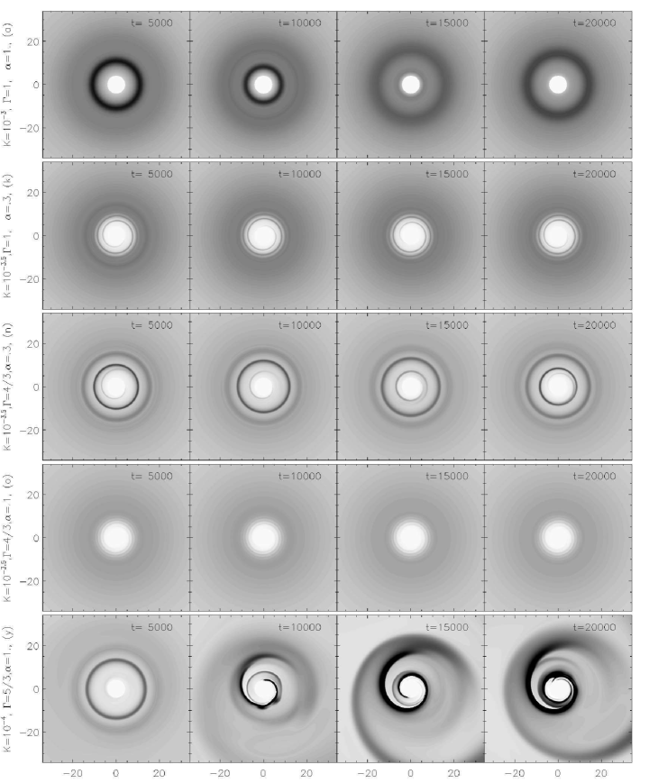
Figure 1.— Density contours for a representative set of parameters $(K,\Gamma,\alpha)$ at different times. The gray scale is linear, with white representing $\Sigma=0$ and black representing $\Sigma=6$. From top to bottom, we have (i) pure axisymmetric waves, (ii) axisymmetric waves interacting with an one-armed spiral, (iii) an one-armed spiral in the inner disk, (iv) two-armed spirals in the inner disk, and finally (v) a turbulent state in the inner disk, and one-armed spiral in the outer disk. See §4 for an overview of these features.

Figure 1 shows a representative set of snapshots from our parameter study. Each row contains four density contours of a particular simulation. The gray scale is linear, with white representing $\Sigma=0$ and black representing $\Sigma=6$. From top to bottom, we can see the five most significant features: (i) A pure axisymmetric mode is excited near the ISCO and propagates outward. (ii) An one-armed spiral develops only at the inner edge, while the other part of the computational domain is stable. (iii) Axisymmetric rings appear and interact with the one-armed spiral at the inner edge. (iv) Two-armed spirals develop at the inner edge when the rest of the disk is stable. Finally, (v) the axisymmetric waves clean up the inner part of the disk. Inner spirals develop in this low density region and perturb the rings. The rings then break apart in late time and go through a turbulent transition state. After that, strong steady trailing spirals develop in the inner disks while global leading spirals develop in the outer disks.

We will discuss these features in more detail in later sections. Nevertheless, to provide a general picture, we review the standard models of thin disk oscillation. Following K01, we consider the small quantity $h_{mn}(r)\sim P^{(1)}/\Sigma^{(0)}$. The subscript $m$ and $n$ indicate different azimuthal and vertical modes, respectively. And $P^{(1)}$ denotes the first order fluctuation in pressure. For simplicity, we will drop the subscripts $m$ and $n$ hereafter. The small quantity $h$ is governed by the equation

$$c_{\mathrm{s}}^{2}\frac{d}{dr}\left(\frac{1}{\tilde{\omega}^{2}-\kappa^{2}}\frac{dh}{dr}\right)+\left(1-\frac{nc_{\mathrm{s}}^{2}}{\tilde{\omega}^{2}H^{2}}\right)h=0,$$ (23)

where $\tilde{\omega}\equiv\omega-m\Omega_{\mathrm{K}}$ and $\kappa$ is the epicyclic frequency (Nowak & Wagoner, 1992).

Assuming the perturbation $h$ is local and has radial wavenumber $k$, the previous equation reduces to a dispersion relation

$$(\tilde{\omega}^{2}-\kappa^{2})(\tilde{\omega}^{2}-n\Omega_{\perp}^{2})=\tilde{\omega}^{2}c_{\mathrm{s}}^{2}k^{2},$$ (24)

where $\Omega_{\perp}=c_{\mathrm{s}}/H=\Omega_{\mathrm{K}}$ is the vertical oscillation frequency. Setting $n=0$ for a two-dimensional disk, the $p$-mode is described by

$$\tilde{\omega}^{2}\equiv(\omega-m\Omega_{\mathrm{K}})^{2}=\kappa^{2}+c_{\mathrm{s}}^{2}k^{2};$$ (25)

while the $g$-mode reduces to a trivial mode

$$\tilde{\omega}\equiv\omega-m\Omega_{\mathrm{K}}=0,$$ (26)

which describes pure rotations. We will argue in §6 that the axisymmetric rings seen in cases (i) and (iii) cannot be described by setting $m=0$ in equation (25). On the other hand, the non-axisymmetric spirals in (ii), (iii), and (iv) can be described by equation (26), while the global spirals are the $m=1$ $p$-modes.

Table 1Summary of results from the parameter study

$K$	$\Gamma$	$\alpha$	Label	Resolutions	$\dot{M}_{\mathrm{ana}}$	$\dot{M}_{\mathrm{num}}$	Init. $\omega_{\mathrm{ring}}$	$\omega_{\mathrm{ring}}$	Init. $\omega_{\mathrm{spiral}}$	$\omega_{\mathrm{spiral}}$	Global Spiral
$10^{-3}$	$1$	$1$	(a)	$129\times 32$	8.603	8.390	$\approx$ 0.02	0.015
$10^{-3}$	$1$	$1^{-0.5}$	(b)	$129\times 32$	2.720	2.525	$\approx$ 0.03	0.028
$10^{-3}$	$1$	$0.1$	(c)	$129\times 32$	0.860	0.767	decay
$10^{-3}$	$4/3$	$1$	(d)	$129\times 32$	11.470	11.223	$\approx$ 0.01	0.012
$10^{-3}$	$4/3$	$1^{-0.5}$	(e)	$129\times 32$	3.627	3.411	$\approx$ 0.03	0.025
$10^{-3}$	$4/3$	$0.1$	(f)	$129\times 32$	1.147	1.032	decay
$10^{-3}$	$5/3$	$1$	(g)	$129\times 32$	14.338	14.049	$\approx$ 0.01	0.009
$10^{-3}$	$5/3$	$1^{-0.5}$	(h)	$129\times 32$	4.534	4.306	$\approx$ 0.02	0.025
$10^{-3}$	$5/3$	$0.1$	(i)	$129\times 32$	1.434	1.297	decay
$10^{-3.5}$	$1$	$1$	(j)	$257\times 64$	2.720	2.635	$\approx$ 0.02	0.021
$10^{-3.5}$	$1$	$1^{-0.5}$	(k)	$257\times 64$	0.860	0.810	$\approx$ 0.03	0.031	$\approx$ 0.10–0.11	0.098
$10^{-3.5}$	$1$	$0.1$	(l)	$257\times 64$	0.272	0.250	decay			0.212
$10^{-3.5}$	$4/3$	$1$	(m)	$257\times 64$	3.627	3.529	$\approx$ 0.02	0.018
$10^{-3.5}$	$4/3$	$1^{-0.5}$	(n)	$257\times 64$	1.147	1.089	$\approx$ 0.03	0.031	$\approx$ 0.09–0.12	$\approx$ 0.01
$10^{-3.5}$	$4/3$	$0.1$	(o)	$257\times 64$	0.363	0.338	decay		$\approx$ 0.21	0.206
$10^{-3.5}$	$5/3$	$1$	(p)	$257\times 64$	4.534	4.425	$\approx$ 0.02	0.018
$10^{-3.5}$	$5/3$	$1^{-0.5}$	(q)	$257\times 64$	1.434	1.367	$\approx$ 0.03	0.028	$\approx$ 0.06–0.15	$\approx$ 0.01
$10^{-3.5}$	$5/3$	$0.1$	(r)	$257\times 64$	0.453	0.425	decay		$\approx$ 0.20	0.202
$10^{-4}$	$1$	$1$	(s)	$513\times 128$	0.860	0.842	$\approx$ 0.02	0.025	decay	weak
$10^{-4}$	$1$	$1^{-0.5}$	(t)	$513\times 128$	0.272	0.264	$\approx$ 0.03	0.031	decay	weak
$10^{-4}$	$1$	$0.1$	(u)	$513\times 128$	0.086	0.082	decay			0.117
$10^{-4}$	$4/3$	$1$	(v)	$513\times 128$	1.147	1.049	$\approx$ 0.02	—	decay	—	steady
$10^{-4}$	$4/3$	$1^{-0.5}$	(w)	$513\times 128$	0.363	0.349	$\approx$ 0.03	—	decay	—	steady
$10^{-4}$	$4/3$	$0.1$	(x)	$513\times 128$	0.115	0.110	decay			0.114
$10^{-4}$	$5/3$	$1$	(y)	$513\times 128$	1.434	0.999	$\approx$ 0.02	—	decay	—	steady
$10^{-4}$	$5/3$	$1^{-0.5}$	(z)	$513\times 128$	0.453	0.229	$\approx$ 0.03	—	decay	—	steady
$10^{-4}$	$5/3$	$0.1$	(@)	$513\times 128$	0.143	0.138	decay		$\approx$ 0.10	0.110

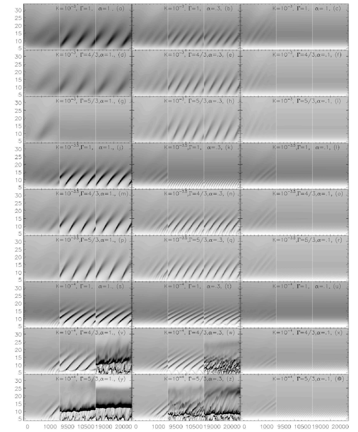
Figure 2.— Column density at $\phi=0$ as contours of $t$ (horizontal axis) and $r$ (vertical axis). The gray scale is linear, with white representing 0 and black representing 6. The horizontal axis is chopped into three segments, namely, the early time $[0,1000]$, middle time $[9500,10500]$, and late time $[19000,20000]$. The high density (dark) features that appear around $r\gtrsim 6$ correspond to the axisymmetric rings. The weaker features that appear around $r\lesssim 12$, with fast temporal variability, are non-axisymmetric spirals.

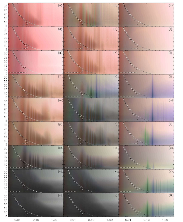
Figure 3.— The power spectra multiplied by $\omega$, i.e., $\omega P(\omega)$, of the density as contours of frequency (horizontal axis) and radius (vertical axis). They are roughly the Fourier transforms of the panels in Figure 2 along the horizontal axis. The order of each panel is the same as in Figure 2. Because the first three azimuthal modes are the most important ones, we can use red, green, and blue to present $m=0$, 1, 2 modes, respectively. Deeper color represents higher power in the logarithmic scale. See §4 and footnote 3 for the details of the coloring scheme. The dotted lines and dashed lines are the Keplerian and epicyclic frequencies, respectively.

In order to give a more quantitative description of the various simulations, we list some important numbers in Table 1. The first three columns are the parameters we explored. The fourth column gives a single letter label to each simulation. The fifth column lists the resolutions. Note that, as we decrease $K$, the kinematic viscosity $\nu_{\mathrm{SS}}$ decreases as well. Higher resolutions are then used to resolve the high Reynolds number flows. The sixth column lists the analytical accretion rate $\dot{M}_{\mathrm{ana}}$ calculated by equation (18); while the seventh column lists the numerical accretion rate $\dot{M}_{\mathrm{num}}$ computed from the simulations,

$$\dot{M}_{\mathrm{num}}=-\frac{1}{T}\int\!\!\!\!\int\Sigma v_{r}r\;dt\;d\phi.$$ (27)

The time integrations are taken between $t=10000$ and 20000 so that $T=10000$. The resulting $\dot{M}_{\mathrm{num}}$ are almost independent of the radius. The values listed in Table 1 are computed at $r=34$, the mid-point of our radial domain, to minimize the boundary effects. The differences between $\dot{M}_{\mathrm{ana}}$ and $\dot{M}_{\mathrm{num}}$ are always less than 10% except for simulations (y) and (z). This agreement, together with the fact that the mean density profiles are well described by our analytical approximations (see next section and Figure 4), imply that our initial conditions are reasonably close to the steady states.

The eighth and ninth columns are the oscillation frequencies of the axisymmetric rings $\omega_{\mathrm{ring}}$. The values in the table are computed at the ISCO although the frequencies are inpendent of the radius in all of our simulations. The eighth column lists rough descriptions of the axisymmetric rings in the early time of the simulations. If the axisymmetric rings decay away before $t=2,000$, we identify them as relaxation effects of the initial conditions and mark “decay” in the table. If the oscillations remain strong at $t=2,000$, we measure the time difference between the density peaks and estimate the frequency by the equation $\omega_{\mathrm{ring}}=2\pi/$period. The values listed in the ninth column are more robust measurements of the frequencies. They are calculated based on (temporal) spectral analysis of the simulations between $t=7,712$ and 20,000. The details can be found in the next section. The symbol “—” indicates the power is distributed across a wide dynamic range, i.e., no specific frequency can be identified. Empty cell indicates the solution is stable so no significant frequency is found.

The tenth and eleventh columns are the oscillation frequencies of non-axisymmetric inner spirals $\omega_{\mathrm{spiral}}$. Note that, due to the interaction between inner spirals and the axisymmetric rings, the spirals do not have a unique frequency in simulations (k), (n), and (q). The differences between the peaks are uneven. We therefore write a frequency range for the estimated frequencies in the tenth column. The eleventh column lists the peak locations for the power spectra. Finally, the last column lists if a steady global spiral appears at late times in the simulations.

5. Temporal Analysis

In order to make the analysis more intuitive, we first plot the column density for each simulation at $\phi=0$ as a contour of radius and time in Figure 2. The time axis is broken into three segments, namely, the early time $[0,1000]$, middle time $[9500,10500]$, and late time $[19000,20000]$. The gray scale is linear, with white representing $\Sigma=0$ and black representing $\Sigma=6$. This is identical to the gray scale used in Figure 1.

For all panels except (v), (w), (y), and (z), the high density (dark) features around $r\gtrsim 6$ correspond to the axisymmetric rings. The slopes of these features, $\delta r/\delta t$, are their (radial) pattern speeds. The weaker features appearing around $r\lesssim 12$ correspond to the non-axisymmetric spirals. Because the angular velocities are almost Keplerian in all simulations, it is easy to identify panels (k), (u), (x), and (@) with one-armed spirals, and panels (l), (o), and (r) with two-armed spirals, simply base on their temporal variability.

Panels (v), (w), (y), and (z) are more complicated. The three time segments show that the properties of the flow are time-dependent. For simulations (v) and (w), the flows are laminar in the first two segments. The extra features that appear around $r\sim 7$ in the middle segment indicate that the axisymmetric rings interact with the very weak inner spirals. These extra features break apart and transit to a turbulent state. The same kind of transition happens in simulations (y) and (z). The almost time independent dark feature at $r\sim 27$ in panel (y) and $r\sim 32$ in panel (z) are the steady global one-armed spirals (see the lowest row of Figure 1).

We follow Kato’s convention and write

$$\Sigma(t,r,\phi)=\sum_{m}\int_{-\infty}^{\infty}\hat{\Sigma}_{m}(\omega,r)\;e^{i(\omega t-m\phi)}\;d\omega,$$ (28)

where $\hat{\Sigma}_{m}(\omega,r)$ is the Fourier transform/coefficient. The power spectrum, defined by

$$P_{m}(\omega,r)\equiv|\hat{\Sigma}_{m}(\omega,r)|^{2},$$ (29)

measures the contribution of different frequencies for a particular azimuthal mode as function of radius. Because the dynamic variables are smooth and periodic along the azimuthal direction, the azimuthal modes are trivial to obtain by applying discrete Fourier transform. However, the variables are not necessary periodic in time, or, at least the exact period is not known before doing the temporal analysis. The PDS obtained by squaring the discrete Fourier transform in a finite time domain (i.e., periodogram) is not a good estimator of the actual power spectrum $P_{m}(\omega,r)$.

In order to improve the statistics, we use the standard “overlap method” (see Press et al., 1992) to average over 11 periodograms. Each periodogram is computed over a section of 2048 snapshots, with two subsequent sections overlapped by 1024 frames. This requires $12\times 1024=12288$ snapshots in total. We drop the first 7712 snapshots in our data to avoid analysing the initial relaxation. The Hann window function is applied to each segment before calculating the periodogram. The resulting variance in the PDS is approximately 11%.

We plot the estimated $\omega P_{m}(\omega,r)$ in Figure 3. The order of the panels are the same as Figure 2. Because only the first few azimuthal modes are important, we can use the red, green, and blue color channels to represent each of them. These three color channels are overlapped in a way that darker color represents a higher power in a logarithmic scale. For example, the red tone for panel (a), (d), and (g) indicates they are purely $m=0$ axisymmetric modes. The brownish color for panel (j), (m), and (p) indicates they are dominated by $m=0$ modes, but have minor contributions from the $m=1$ modes. The dark gray in panel (s), (v), and (y) indicates all $m=0$, 1, and 2 modes contribute. The sharp green and blue lines in panel (l), (o), (r), (u), (x), and (@) correspond to the fundamental modes and overtones of the one-armed and two-armed spirals, respectively.

In addition, the dashed lines in Figure 3 are the epicyclic frequency $\kappa(r)$ and the dotted lines are the Keplerian frequency $\Omega_{\mathrm{K}}$ in pseudo-Newtonian gravity. In contrast to the standard assumption, the oscillations in our simulations are not locally sub-Keplerian. Instead, the angular frequencies of both the axisymmetric rings and the non-axisymmetric spirals are independent of the radius (see Mao et al., 2008). Their values are listed in the ninth and eleventh columns in Table 1.

6. Axisymmetric Rings

If the axisymmetric rings were only seen in our spectral algorithm, one would worry that they may be due to numerical artifacts of our code. The fact that these oscillations were seen in previous studies of viscous spreading rings (Papaloizou & Stanley, 1986; Okuda & Mineshige, 1991; Okuda et al., 1992; Godon, 1995) as well as viscous disk models (Okuda et al., 1992; Chen & Taam, 1992, 1995; Milsom & Taam, 1996; Mao et al., 2008; Reynolds & Miller, 2008) suggest they are likely to be physical, at least under the thin disk assumption. Recently, Reynolds & Miller (2008) performed a detailed temporal analysis of both hydrodynamic and magnetohydrodynamic simulations. For their inviscid hydrodynamic simulations, similar axisymmetric oscillations are seen in the mid-plane, although the authors associate them with the $g$-modes. We are also aware of the current study of oscillations in tilted magnetohydrodynamic disks by Henisey & Blaes (private communication).

Analytical studies of radial oscillations of axisymmetric modes in accretion disks have a long history. Blumenthal et al. (1984) studied the overstability of axisymmetric oscillations and Lubow & Pringle (1993) studied axisymmetric wave propagation in accretion disks. A detailed analytical study of the generation and propagation of these waves is beyond the scope of this paper. However, a simple comparison suggests that more physics is needed in the standard model, i.e., Kato (2001), hereafter K01, in order to describe wave propagation in thin disks.

Note that, when $\omega_{\mathrm{ring}}$ is well defined, it is always smaller than the maximum epicyclic frequency $\kappa_{\mathrm{max}}\equiv\kappa(r_{\mathrm{peak}})\approx 0.0347$, where $r_{\mathrm{peak}}=2(2+\sqrt{3})$. This suggests the axisymmetric rings are generated as inertial waves and then propagate outward. Recalling the dispersion relation for axisymmetric inertial acoustic wave is $\omega^{2}=\kappa^{2}+c_{\mathrm{s}}^{2}k^{2}$, because $k^{2}>0$ and the disk is thin, $c_{\mathrm{s}}^{2}k^{2}\ll\Omega_{\perp}^{2}\sim\kappa^{2}$, it leads to a constraint on the local oscillation frequency $\omega\gtrsim\kappa$. Therefore, K01 argue that a wave with frequency $\omega_{\mathrm{ring}}<\kappa_{\mathrm{max}}$ cannot propagate in the region $[r_{1},r_{2}]$, where $r_{1}$ and $r_{2}$ are the Lindblad resonance points satisfying $\omega_{\mathrm{ring}}=\kappa(r)$. If the wave is excited far out and propagates inward, its wavelength becomes infinite at $r_{2}$ and is reflected back out. On the other hand, if the wave is excited near the inner edge of the disk, it will be reflected back and forth between the inner edge and $r_{1}$. This phenomenon is called wave trapping.

Taking simulation (j) as an example, $\omega_{\mathrm{ring}}=0.021$. The standard picture predicts no wave can propagate within the region $[r_{1},r_{2}]=[6.203,12.587]$; waves should be trapped between the inner edge (near the ISCO) and $r_{1}$. Panel (j) in Figure 3 clearly contradicts this prediction and violates the constraint $\omega\gtrsim\kappa$. Indeed, the power at the dominant mode increases in the forbidden region $[r_{1},r_{2}]$, and extends far to the outer region. K01 commented that the physical reasons for the difference between analytical models and numerical simulations are not clear.

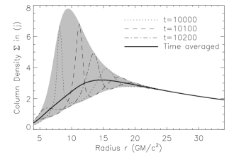
Figure 4.— Typical density profiles at $\phi=0$. The dotted line, dashed line, and dashed-dotted lines are profiles taken at $t=10000$, $10100$, and $10200$, respectively. The thick solid line is the time average between $t=10000$ and $20000$. The gray area marks the maximums and minimums of the waves.

In Figure 4, we plot the density profile of simulation (j) at $\phi=0$. The different dashed and dotted lines are profiles taken at $t=10000$, $10100$, and $10200$. The thick solid line is the time average between $t=10000$ and $20000$. The gray area marks the maximums and minimums of the waves. The amplitudes of the oscillations (for this particular simulation) are not small compared to the background. The peak is located around $r=9.5$, with peak densities about four times the mean density. Also, the wavelengths are comparable to the radius, i.e, $k\sim 1/r$.

To compare how the amplitudes vary with the parameters, we plot the quantity $|{\max}(\Sigma)/\langle\Sigma\rangle-1|^{2}\sim|{h}|^{2}$ in Figure 5. The solid, dotted, and dashed lines correspond to simulations (a), (j), and (s), respectively. The fluctuations in simulation (a) decays exponentially as a function of $r$. As the pressure decrease, like in cases (j) and (s), the fluctuations become nonlinear and the decay rates increase.

There are two kinds of difficulties in applying the standard thin disk oscillation modes. First, as shown in Figure 4, the local linear approximation breaks down due to the non-linearity and large wavelength of the axisymmetric waves. Second, even in the cases where local linear approximation is valid [say simulation (a)], Figure 5 shows the fluctuations are damped in large radii, hence the wavenumber $k$ is complex. The standard approach, i.e., equation (23), does not take this into account. More physics perhaps related to viscosity should be included in the linear mode analysis in order to understand the wave generation and propagation.

Figure 5.— The function $|{\max}(\Sigma)/\langle\Sigma\rangle-1|^{2}\sim|h|^{2}$ plotted in log scale taken from the period $t=10000$ to 20000. The solid line is for simulation (a), the dotted line for (j), and the dashed line for (s). When the amplitude is small, i.e., for simulation (a), the fluctuation decays exponentially for $r\gtrsim 10$.

7. Non-Axisymmetric Inner Spirals

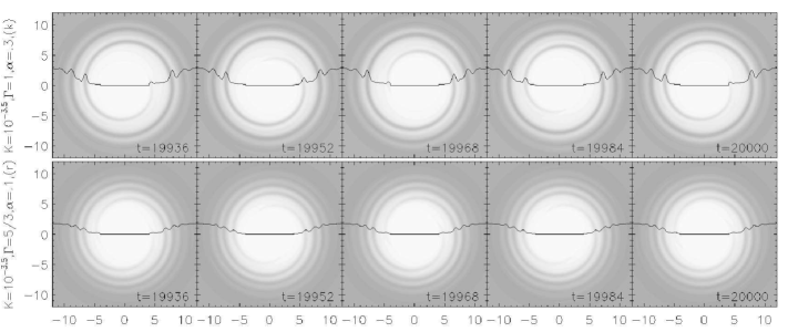
Figure 6.— Close up view of the central one-armed (top) and weak two-armed (bottom) spirals. The gray scale is linear in both rows with white representing $\Sigma=0$. Black represents $\Sigma=9$ for the top row and $\Sigma=6$ for the bottom row. The time difference between each frame is 16, which is about a quarter of a period at the ISCO. Hence, the contours at $t=19936$ is pretty much the same as $t=20000$ because the flows rotate a full period. The solid lines show the column density along the horizontal axis, with the vertical axis matching the numerical values. The solid lines for the bottom row are symmetric because of the $m=2$ modes.

Linear stability analysis of hydrodynamic disks was an active area of study in the 1980’s. Papaloizou & Pringle (1984, 1985), Goldreich & Narayan (1985) and Papaloizou & Pringle (1987) showed that inviscous tori are unstable to non-axisymmetric perturbations. The global analysis was extended by Blaes (1985), Goldreich et al. (1986), and Goodman et al. (1987); while Narayan et al. (1987) performed a local analysis based on the shearing sheet approximation. Self-gravity was included in Goodman & Narayan (1988), and Papaloizou & Lin (1988) showed that, if the effective viscous stress is a rapidly increasing function of the column density, non-axisymmetric perturbations grow because of viscous overstability.

Table 1 shows that for one-armed spirals, $\omega_{\mathrm{spiral}}$ is always very close to the Keplerian frequency at the ISCO, $\Omega_{\mathrm{K}}(r_{\mathrm{ISCO}})\approx 0.102$; while for two-armed spirals $\omega_{\mathrm{spiral}}\approx 2\Omega_{\mathrm{K}}(r_{\mathrm{ISCO}})$. This observation strongly suggests that inner spirals are generated by corotating density fluctuations, which can be described by the trivial mode at the ISCO. The density fluctuations spiral inward as the SPBF suggests and create the rotating patterns in the inner disks.

In Figure 6, we plot the contours of the very central region of two simulations that have inner spirals but no significant axisymmetric rings. The gray scale is again linear, with white representing $\Sigma=0$. Black represents $\Sigma=9$ for the top row [simulation (k) with an one-armed spiral] and $\Sigma=6$ for the bottom row [simulation (r) with two-armed spirals]. The time difference between each snapshot is 16, which is about a quarter of a period at the ISCO. Therefore, the contours at $t=19936$ look almost identical to the contours at $t=20000$.

The solid lines in Figure 6 show the amplitudes of the column density $\Sigma$ along the horizontal axis with the values matching the vertical axis. The amplitudes are parameter dependent. For example, the spirals have non-linear amplitudes for simulation (k); while for simulation (r), the amplitude is small, so perturbation methods are applicable. This result is consistent with the analytical study of Papaloizou & Lin (1988), in the sense that the amplitude of the spirals is an increasing function of $\Gamma$. Also note that the solid lines are symmetric (because of the $m=2$ mode) for the bottom row.

8. Transient and Steady Global Spirals

Kato (1983) showed that one-armed inertial-acoustic waves (with $n=0$), which are just an eccentric deformation of the disk plane, have frequencies much lower than $\Omega_{\mathrm{K}}$. Ogilvie unified a number of efforts (see reference in Ogilvie, 2001) and derived a comprehensive set of evolutionary equations for eccentric disks. Later, Speith & Kley (2003) performed a careful perturbation analysis and showed that the perturbations are independent of the dynamical time scales. These types of (almost) steady global spiral patterns are believed to be the cause of the V/R variations of Be stars (see K01 and reference therein).

Following Kato (1983), we consider the $p$-mode dispersion relation (25) with $m=1$,

$$\omega=\Omega_{\mathrm{K}}\pm\sqrt{\kappa^{2}+c_{\mathrm{s}}^{2}k^{2}}.$$ (30)

For nearly Keplerian disks, $\kappa\approx\Omega_{\mathrm{K}}$. If the disk is thin and the oscillation is global, i.e., $c_{\mathrm{s}}k\ll\Omega_{\mathrm{K}}$, the lower frequency can be approximated by

$$\omega\approx\Omega_{\mathrm{K}}-\sqrt{\Omega_{\mathrm{K}}^{2}+c_{\mathrm{s}}^{2}k^{2}}\approx\frac{1}{2}\Omega_{\mathrm{K}}\left(\frac{c_{\mathrm{s}}k}{\Omega_{\mathrm{K}}}\right)^{2}\ll\Omega_{\mathrm{K}}.$$ (31)

Hence, for a simulation with a small enough sound speed, we expect our numerical solution to evolve to a state that agrees with the above analytical result.

Form the bottom panels of Figure 1, we can briefly see the different stage of such an evolution. When $t\lesssim 5000$, axisymmetric waves are excited and clean up the inner part of the disk. Spiral structures can form in this very low density region. The inner spirals interact with the axisymmetric rings. At $t\sim 10000$, if the Reynolds numbers are high enough [simulation (v), (w), (y), and (z)], both the axisymmetric rings and the inner spirals are able to break apart. The inner disks then go through a turbulent transition state. Although the turbulent transient states are potentially very important, we cannot draw strong conclusions from them. This is because these high Reynolds number flows are barely resolved even with $513\times 128$ grids. Other concerns include the inner boundary effects (see McKinney & Gammie, 2002) and some numerical issues are discussed in the next section. Nevertheless, the strong trailing spirals that develop in the inner disks and the global leading spirals develop in the outer disks later on are very robust features.

To focus on the trailing spirals, we plot the contours of the central region of simulation (x) and (z) in Figure 7. The contours are plotted using the same time scale as Figure 6 for easy comparison. The gray scale is again linear, with white representing $\Sigma=0$ and black representing $\Sigma=18$ for both rows. The solid lines show the column density along the horizontal axis, which show the spirals are very non-linear. Note that the spirals patterns are almost independent of time, as suggested in Kato (1983) and summarized in equation (31).

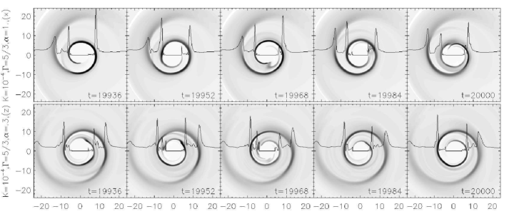
Figure 7.— Close up view of the central strong one-armed spirals found in both simulation (x) [top row] and (z) [bottom row]. The contours are plotted at the same time as in Figure 6 for easy comparison. Note that the spirals patterns are almost independent of time, as suggested in Kato (1983). The gray scale is again linear, with white representing $\Sigma=0$ and black representing $\Sigma=18$ for both rows. The solid lines show the column density along the horizontal axis, which show the spirals are very non-linear.

9. Limitations

Accretion disks involve different physics at different scales are very complicated systems. Although we have presented results based on careful numerical studies, one needs to be aware of the limitations in the simulations. In this section, we provide a list of some important concerns we have, and suggest several possible improvements for future studies.

There are several numerical limitations that we need to be aware of. First, for the high Reynolds number cases, although $513\times 128$ grid points are used, we can barely resolve the accretion flows. Our artificial viscosity may then have important effects on the flows, even though they are high order. Second, in some of our simulations, the axisymmetric rings (together with the inflow, of course) clean up the inner region of the accretion disks. The density is so low that a density floor is often used to prevent negative values. Because this only happen in the inner region, it is likely that the artificially introduced mass would fall towards the central object very quickly. However, it is not clear to us how important this effect is on the properties of our numerical solutions. Third, because we used an explicit Eulerian algorithm, the time steps are extremely small due to the fast flow and small grid at the inner boundary. Our high resolution simulations use more than a million time steps. The culmination of both truncation and round off errors may start polluting our numerical solutions.

The above concerns suggest that, although the turbulent transient states found in our high Reynolds number simulations [i.e., (v), (w), (y), and (z)] are potentially important, one should not draw strong conclusions from them. Better numerical algorithms with higher resolutions are needed to study them.

In addition to the numerical issues, there are problems associated with non-general relativistic hydrodynamics. McKinney & Gammie (2002) performed a careful study of two-dimensional (in $r$-$z$ plane) viscous hydrodynamic disks. They pointed out that numerical solutions in pseudo-Newtonian gravity depend on the location of the inner boundary. In our simulations, because the chosen sound speeds are small, the flows at the inner boundary are super-sonic. The boundary effect is therefore not important. Nevertheless, a general relativity version of our code will improve the numerical solutions and lead to more confident results. However, there is no unique way to formulate relativistic hydrodynamics with viscosity. Methods like using flux-limited diffusion (Wilson & Mathews, 2003), or including an explicitly defined “finite time propagator” (Koide et al., 2007), are proposed.

Finally, we have completely neglected the effect of magnetic fields and adopted the $\alpha$-viscosity prescription. It is well known that MHD turbulence in thick disk simulations tend to destroy coherent structures and wash away periodic signatures. Moreover, Pessah et al. (2008) pointed out that magnetorotational instability (MRI) driven turbulence does not behave like $\alpha$-viscosity. It is not clear whether equation (1) and (2) can capture the correct dynamics of accretion flows, even within a thin disk approximation. A study of oscillations from MHD simulations of tilded disks [Henisey & Blaes (private communication)] and thin MHD disks (Shafee et al., 2008) will therefore be very interesting.

10. Discussions

In this paper, we have performed a parameter study of two-dimensional viscous accretion disks. We have found three types of robust features: the axisymmetric rings, the non-axisymmetric inner spirals, and the steady global one-armed spirals. When applying a temporal analysis of the column density, a large amount of power is contained in a few modes with frequencies that are independent of the radius.

Although the properties of the axisymmetric rings do not completely agree with theoretical predictions, the frequencies $\omega_{\mathrm{ring}}$ are always smaller than the maximum epicyclic frequency $\kappa_{\mathrm{max}}$. This strongly suggests that they are axisymmetric $p$-modes. By taking a closer look at the simulations, we find out that the local, linear assumption breaks down in the inner disk. Moreover, based on the results of the simulations, we argue that the standard linear mode analysis is not enough to understand these rings. The fact that these inertial acoustic modes can propagate to large radii with constant frequencies have important implications — a frequency found in an observed oscillation can correspond to a large range of radii in the accretion disks. Therefore, one cannot use it to estimate the size of the emission region (see Mao et al., 2008, for related discussions).

The two types of non-axisymmetric modes have very different properties. For the inner spirals, their frequencies are always very close to a small multiple of the Keplerian frequency at the ISCO, $m\Omega_{\mathrm{K}}(r_{\mathrm{ISCO}})$. Hence, they simply are rotating patterns originating at the ISCO and corresponding to the trivial $g$-mode $\tilde{\omega}=0$. The formation of the $m=1$ and $m=2$ modes is probably due to viscous overstability.

Although there are some situations in which both the axisymmetric rings and the non-axisymmetric spirals co-exist, the connection between these two features is not entirely clear. The excitation of rings usually cleans up the inner disks and prevents the inner spirals to develop. However, there are cases in which that the inner spirals perturb the axisymmetric rings. Steady global spirals are then excited. These steady patterns have properties that agree with the low frequency global $m=1$ $p$-modes. They are predicted as general features when the disks weakly deviated from Keplerian and have slow sound speed (K01). The same feature can also be understood as eccentric deformation.

Modeling if QPOs can roughly be classified into two major schools. One conjectures that the observed oscillations correspond to the eigenfrequencies in the accretion disks. The other proposes that an inspiral stream of matter is responsible for the modulation. Our simulations show, depending on the parameter, both features can be excited in viscous disks. Although the two frequencies are associated with axisymmetric rings and inner spirals are in ratio 1:3 instead of the observed 2:3, our results provide new insights to understand and model QPOs.

References

- Abramowicz & Kluźniak (2001) Abramowicz, M. A., & Kluźniak, W. 2001, A&A, 374, L19
- Blaes (1985) Blaes, O. M. 1985, MNRAS, 216, 553
- Blumenthal et al. (1984) Blumenthal, G. R., Lin, D. N. C., & Yang, L. T. 1984, ApJ, 287, 774
- Chan et al. (2005) Chan, C.-K., Psaltis, D., & Özel, F. 2005, ApJ, 628, 353
- Chen & Taam (1992) Chen, X., & Taam, R. E. 1992, MNRAS, 255, 51
- Chen & Taam (1995) —. 1995, ApJ, 441, 354
- Frank et al. (2002) Frank, J., King, A., & Raine, D. J. 2002, Accretion Power in Astrophysics: Third Edition (Accretion Power in Astrophysics, by Juhan Frank and Andrew King and Derek Raine, pp. 398. ISBN 0521620538. Cambridge, UK: Cambridge University Press, February 2002.)
- Godon (1995) Godon, P. 1995, MNRAS, 274, 61
- Goldreich et al. (1986) Goldreich, P., Goodman, J., & Narayan, R. 1986, MNRAS, 221, 339
- Goldreich & Narayan (1985) Goldreich, P., & Narayan, R. 1985, MNRAS, 213, 7P
- Goodman & Narayan (1988) Goodman, J., & Narayan, R. 1988, MNRAS, 231, 97
- Goodman et al. (1987) Goodman, J., Narayan, R., & Goldreich, P. 1987, MNRAS, 225, 695
- Kato (1983) Kato, S. 1983, PASJ, 35, 249
- Kato (2001) —. 2001, PASJ, 53, 1
- Kato (2004) —. 2004, PASJ, 56, 905
- Kato (2008a) —. 2008a, PASJ, 60, 111
- Kato (2008b) —. 2008b, ArXiv e-prints, 808
- Kluzniak & Abramowicz (2001) Kluzniak, W., & Abramowicz, M. A. 2001, Acta Physica Polonica B, 32, 3605
- Koide et al. (2007) Koide, T., Denicol, G. S., Kodama, T., & Mota, P. 2007, Brazilian Journal of Physics, 37, 1047
- Lubow & Pringle (1993) Lubow, S. H., & Pringle, J. E. 1993, ApJ, 409, 360
- Ma (1998a) Ma, H. 1998a, SIAM J. Numer. Anal., 35, 869
- Ma (1998b) —. 1998b, SIAM J. Numer. Anal., 35, 893
- Mao et al. (2008) Mao, S. A., Psaltis, D., & Milsom, J. A. 2008, ArXiv e-prints, 805
- McKinney & Gammie (2002) McKinney, J. C., & Gammie, C. F. 2002, ApJ, 573, 728
- Milsom & Taam (1996) Milsom, J. A., & Taam, R. E. 1996, MNRAS, 283, 919
- Narayan et al. (1987) Narayan, R., Goldreich, P., & Goodman, J. 1987, MNRAS, 228, 1
- Nowak & Wagoner (1992) Nowak, M. A., & Wagoner, R. V. 1992, ApJ, 393, 697
- Ogilvie (2001) Ogilvie, G. I. 2001, MNRAS, 325, 231
- Okuda & Mineshige (1991) Okuda, T., & Mineshige, S. 1991, MNRAS, 249, 684
- Okuda et al. (1992) Okuda, T., Ono, K., Tabata, M., & Mineshige, S. 1992, MNRAS, 254, 427
- Ortega-Rodríguez et al. (2002) Ortega-Rodríguez, M., Silbergleit, A. S., & Wagoner, R. V. 2002, ApJ, 567, 1043
- Papaloizou & Lin (1988) Papaloizou, J. C. B., & Lin, D. N. C. 1988, ApJ, 331, 838
- Papaloizou & Pringle (1984) Papaloizou, J. C. B., & Pringle, J. E. 1984, MNRAS, 208, 721
- Papaloizou & Pringle (1985) —. 1985, MNRAS, 213, 799
- Papaloizou & Pringle (1987) —. 1987, MNRAS, 225, 267
- Papaloizou & Stanley (1986) Papaloizou, J. C. B., & Stanley, G. Q. G. 1986, MNRAS, 220, 593
- Perez et al. (1997) Perez, C. A., Silbergleit, A. S., Wagoner, R. V., & Lehr, D. E. 1997, ApJ, 476, 589
- Pessah et al. (2008) Pessah, M. E., Chan, C.-K., & Psaltis, D. 2008, MNRAS, 383, 683
- Press et al. (1992) Press, W. H., Teukolsky, S. A., Vetterling, W. T., & Flannery, B. P. 1992, Numerical recipes in C. The art of scientific computing (Cambridge: University Press, —c1992, 2nd ed.)
- Psaltis (2004) Psaltis, D. 2004, in American Institute of Physics Conference Series, Vol. 714, X-ray Timing 2003: Rossi and Beyond, ed. P. Kaaret, F. K. Lamb, & J. H. Swank, 29–35
- Psaltis et al. (2008) Psaltis, D., Perrodin, D., Dienes, K. R., & Mocioiu, I. 2008, Physical Review Letters, 100, 091101
- Remillard & McClintock (2006) Remillard, R. A., & McClintock, J. E. 2006, ARA&A, 44, 49
- Reynolds & Miller (2008) Reynolds, C. S., & Miller, M. C. 2008, ArXiv e-prints
- Shafee et al. (2008) Shafee, R., McKinney, J. C., Narayan, R., Tchekhovskoy, A., Gammie, C. F., & McClintock, J. E. 2008, ArXiv e-prints
- Shakura & Syunyaev (1973) Shakura, N. I., & Syunyaev, R. A. 1973, A&A, 24, 337
- Silbergleit et al. (2001) Silbergleit, A. S., Wagoner, R. V., & Ortega-Rodríguez, M. 2001, ApJ, 548, 335
- Speith & Kley (2003) Speith, R., & Kley, W. 2003, A&A, 399, 395
- van der Klis (2000) van der Klis, M. 2000, ARA&A, 38, 717
- van der Klis (2006) —. 2006, Rapid X-ray Variability (Compact stellar X-ray sources), 39–112
- Wagoner (2008) Wagoner, R. V. 2008, New Astronomy Review, 51, 828
- Wilson & Mathews (2003) Wilson, J. R., & Mathews, G. J. 2003, Relativistic Numerical Hydrodynamics (Relativistic Numerical Hydrodynamics, by James R. Wilson and Grant J. Mathews, pp. 232. ISBN 0521631556. Cambridge, UK: Cambridge University Press, December 2003.)