Exploring the Star Formation History of Elliptical Galaxies: Beyond Simple Stellar Populations with a New Line Strength Estimator

Abstract

We study the stellar populations of a sample of 14 elliptical galaxies in the Virgo cluster. Using spectra with high signal-to-noise ratio (S/N$\lower 2.15277pt\hbox{$\;\buildrel>\over{\sim}\;$}100$Å ^-1) we propose an alternative approach to the standard side-band method to measure equivalent widths (EWs). Our Boosted Median Continuum is shown to map the EWs more robustly than the side-band method, minimising the effect from neighbouring absorption lines and reducing the uncertainty at a given signal to noise ratio. Our newly defined line strengths are more sucessful at disentangling the age-metallicity degeneracy. We concentrate on Balmer lines (H$\beta$,H$\gamma$,H$\delta$), the G band and the combination [MgFe] as the main age and metallicity indicators. We go beyond the standard comparison of the observations with simple stellar populations (SSP) and consider four different models to describe the star formation histories, either with a continuous star formation rate or with a mixture of two different SSPs. These models improve the estimates of the more physically meaningful mass-weighted ages. Composite models are found to give more consistent fits among individual line strengths and agree with an independent estimate using the spectral energy distribution. A combination of age and metallicity-sensitive spectral features allows us to constrain the average age and metallicity. For a Virgo sample of elliptical galaxies our age and metallicity estimates correlate well with stellar mass or velocity dispersion, with a significant threshold around $5\times 10^{10}M_{\odot}$ above which galaxies are uniformly old and metal rich. This threshold is reminiscent of the one found by Kauffmann et al. in the general population of SDSS galaxies at a stellar mass $3\times 10^{10}M_{\odot}$. In a more speculative way, our models suggest that it is formation epoch and not formation timescale what drives the Mass-Age relationship of elliptical galaxies.

1 Introduction

Unveiling the star formation histories of elliptical galaxies is key to our understanding of galaxy formation. Being able to resolve their seemingly homogenous distribution is hampered by the fact that their light is dominated by old, i.e. low-mass stars, which do not evolve significantly even over cosmological times. Furthermore, the presence of small amounts of young stars as recently discovered in NUV studies (Ferreras & Silk, 2000; Yi et al., 2005; Kaviraj et al., 2007) reveals a complex history of star formation that requires proper estimates of mass-weighted ages, in contrast with the luminosity-weighted ages that simple stellar populations (SSPs) can only achieve. The majority of papers dealing with age estimates of the stellar populations of elliptical galaxies rely on such SSPs (see e.g. Kuntschner & Davies, 1998; Trager et al., 2000; Thomas et al., 2005), and it is only recently that special emphasis has been made on the need to go beyond simple populations (Ferreras & Yi, 2004; Serra & Trager, 2007; Idiart et al., 2007)

Dating the (old) stellar populations of elliptical galaxies has been fraught with difficulties, the most prominent being the age-metallicity degeneracy, whereby the photo-spectroscopic properties of a galaxy of a given age and metallicity can be replicated by a younger or older galaxy at a suitably higher or lower metallicity, respectively. To some extent, this problem has been overcome by the measurement of pairs of absorption line indices (Worthey, 1994), one whose change in equivalent width (EW) is dominated by the average metallicity of the population and the other dominated by the average age of the population. Typical metal-sensitive line strengths are the Mg feature at 5170Å , the iron lines around 5300Å, or a combination such as [MgFe] (González, 1993). Balmer lines are more age-sensitive and are often combined with metal-sensitive lines to break the degeneracy. However, measurements of EWs of Balmer lines can be affected by the age-metallicity degeneracy because of the presence of nearby absorption lines. Such is the case of H$\gamma$, with the prominent G band at 4300Å or the CN bands in the vicinity of the H$\delta$ line. This paper is partly motivated by the need to define a method to estimate EWs that minimise the sensitivity of metallicity on Balmer lines by a proper estimate of the continuum.

Even at relatively younger ages (a few Gyr) where such uncertainties are reduced, considerable degeneracies still remain. The confirmation of recent star formation (RSF) occuring in early type galaxies (Yi et al., 2005; Kaviraj et al., 2007) has raised the problem that the existence of a young population can considerably affect the parameters derived through SSP analysis. Trager et al. (2000) and later Serra & Trager (2007) showed that even relatively small mass fractions ($\sim$1%) of young stars can distort age and metallicity estimates and in moderate cases ($\sim$10%) completely overshadow the older population. In addition, the age and mass fraction of any younger sub-population will also be degenerate, with larger mass fraction of relatively older sub populations having the same effect as smaller fractions of younger ones.

Schiavon et al. (2004) noticed that using different Balmer lines (H$\beta$, H$\gamma$ and H$\delta$) to estimate the age gives slightly different results, which was suggested to show that the galaxy had undergone recent star formation. Contrary to this, Thomas et al. (2004) find that H$\gamma$ and H$\delta$ equivalent widths are more affected by a non-solar $\alpha$/Fe ratio on higher order Balmer lines. This effect is due to the increase of metal lines at bluer wavelengths, thereby distorting the continuum as measured by a side-band method. This was expanded by Serra & Trager (2007) who remodelled synthetic 2-burst models using H$\beta$ and H$\gamma_{A}$ and achieved a result consistent with both papers, concluding that a mistmatch between the three Balmer line estimates could possibly reveal underlying younger populations.

Moving forward with such analysis – beyond simple populations and luminosity-weighted parameters – requires improvements on both the H$\gamma$ and H$\delta$ measurements. Balmer line equivalent widths suffer from the effects of the metallicity due to the presence of such lines in the spectral region used to determine the continuum (Worthey & Ottaviani, 1997; Thomas et al., 2004; Prochaska et al., 2007). Although considerable work has already been done in this area (see e.g. Rose et al., 1994; Jones & Worthey, 1995; Vazdekis & Arimoto, 1999; Yamada et al., 2006), we test a completely different approach.

In this paper we present a comprehensive analysis of the stellar populations of 14 Virgo cluster ellipticals using several models to describe the star formation history, exploring the discrepancies found between simple and composite stellar populations. In an attempt to combat the problems discussed above, we introduce a new method for the measurement of equivalent widths using a high percentile running “median” to describe the continuum. The properties of this new method are exploited by using various age- and metallicity-sensitive spectral features.

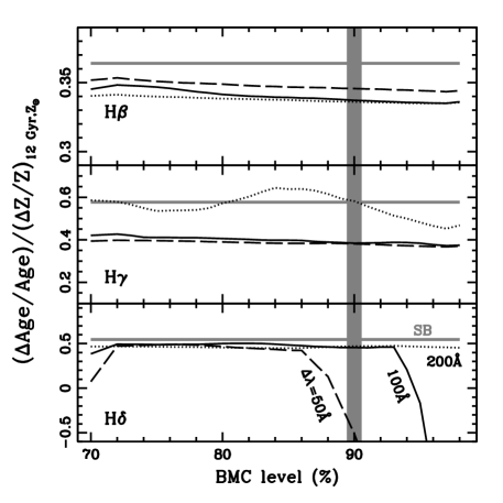
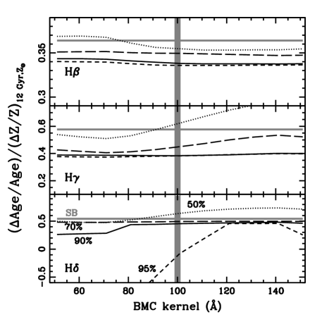
Figure 1: Dependence of the age-metallicity gradient – ($\Delta$ Age/Age)(/$\Delta$ Z/Z) – on the choice of BMC parameters, namely the level at which the ’boosted median’ is taken (left) or the size of the kernel (right). On the left panel a number of kernel sizes is shown as labelled: $\Delta\lambda$=50Å (dashed); 100Å (solid) and 200Å (dotted). On the right panel a number of confidence levels are considered: 50% (dotted); 70% (long dashed); 90% (solid) and 95% (short dashed). The grey horizontal line in both panels is the estimate from the standard side-band method (SB), and the grey vertical shaded area marks our choice of ’boosted median’ parameters.

2 The sample

We use a sample of 14 elliptical galaxies in the Virgo cluster, for which moderate resolution spectroscopy is available at high signal-to-noise ratio (S/N$\;\buildrel>\over{\sim}\;$100 Å^-1, Yamada et al., 2006, 2008). Eight galaxies were observed with FOCAS at the 8m Subaru telescope; the other six were observed with ISIS at the 4.2m William Herschel Telescope (WHT). Observations from Subaru span the spectral range $\lambda\simeq 3800-5800$Å , whereas the spectra taken at the WHT span a narrower window, namely $\lambda\simeq 4000-5500$Å . The resolution (FWHM) of both data sets is similar: 2Å (Subaru) and 2.4Å(WHT). We refer the interested reader to Yamada et al. (2006) for details about the data reduction process. We compare those spectra with composites of the R$\sim 2000$ synthetic models of Bruzual & Charlot (2003), updated to the 2007 version (Bruzual, 2007). We resampled the observed spectra from the original 0.3Å to 1Å per pixel, performing an average of the spectra over a 1.5Å window, in order to have a sampling more consistent with the actual resolution.

In this paper we use two alternative sets of information, either the full spectral energy distribution or targeted absorption lines. For the former, we consider a spectral window around the 4000Å break, which is a strong age indicator (albeit with a significant degeneracy in metallicity, especially for evolved stellar populations). In order to minimise the effect of an error in the flux calibration, we do not choose the full spectral range of the spectra, restricting the analysis to 3800–4500Å  for the Subaru spectra, and 4000–4500Å for the WHT spectra.

The second method focuses on a reduced number of spectral lines. Following the traditional approach (see e.g. Kuntschner & Davies, 1998; Trager et al., 2000; Thomas et al., 2005; Sánchez-Blázquez et al., 2006), we use a set of age-sensitive and metallicity-sensitive lines. In the next section we describe in detail the indices targeted by our analysis and describe a new algorithm that improves on the “standard” method to determine the continuum in galaxy spectra.

3 Measuring Equivalent Widths

We focus on a reduced set of absorption lines originally defined in the Lick/IDS system (Worthey et al., 1994) and extensions thereof (Worthey & Ottaviani, 1997). As age-sensitive lines we use the Balmer lines H$\beta$, H$\gamma$, H$\delta$, the G-band (G4300) and the 4000Å break (D4000). We use the standard definition of [MgFe] (González, 1993), as a metal-sensitive tracer, which is a reliable proxy of overall metallicity, with a very mild dependence on [$\alpha$/Fe] abundance ratio (Thomas et al., 2003).

The standard method to determine the equivalent widths of galaxy spectra relies on the definition of a blue and a red side-band to determine the continuum. A linear fit to the average flux in the blue and red side-bands is used to track the continuum in the line (see e.g. Trager et al., 2000). This method, although easy to implement, has an important drawback as neighbouring lines can make a significant contribution to the flux in the blue and red passbands, introducing unwanted age/metallicity effects. For instance, the H$\gamma$ index (Worthey & Ottaviani, 1997) is defined with the blue side-band located close to the prominent G-band, around 4300Å. This definition causes non-physical negative values of the H$\gamma$ line in absorption, as the depression caused by the G-band makes the flux in the $H\gamma$ line (wrongly) appear in emission. This has not prevented the community from using this line as a sensitive age tracer, as long as models and data are treated in the same way. Vazdekis & Arimoto (1999) defined new measurements of this line in order to reduce the metallicity degeneracy mainly introduced by the choice of the side bands. They avoid this by selecting specific regions less affected by the metal absorption lines.

H$\delta$ is another Balmer line which has been recently considered to be affected by neighbouring metal lines – most notably the CN molecular bands – which reduce the age sensitivity of the index (Prochaska et al., 2007).

In this paper we present an alternative method to determine the equivalent widths. Our method does not rely on the definition of blue and red side-bands and minimizes the contamination from neighbouring lines. This method is simple to apply and we propose it for future studies of stellar populations in galaxies.

3.1 The Boosted Median Continuum (BMC)

Our measure of equivalent width follows the standard procedure comparing observed flux in the line and the corresponding “interpolated” continuum in the same wavelength range. For an equivalent width measured in Å:

$$EW=\int_{\lambda_{1}}^{\lambda_{2}}\Big{[}1-\frac{\Phi(\lambda)}{\Phi_{C}(\lambda)}\Big{]}d\lambda,$$ (1)

where $\lambda_{1}$ and $\lambda_{2}$ define the wavelength range of the line, $\Phi(\lambda)$ is the observed flux, and $\Phi_{C}(\lambda)$ is the flux from the continuum. Rather than defining the continuum as a linear fit between a blue and a red side-band, we propose the “boosted median” of the flux, defined at each wavelength as the 90th percentile of the flux values within a 100Å window.

This method is defined by two parameters, namely the choice of percentile (90% in our case) and the size of the kernel ($\Delta\lambda=$100Å). The kernel size needs to be large enough to avoid the small scale variations of the spectra, but small enough to avoid distortions from large scale structure of the spectra such as the breaks at 4000Å and 4300Å, or flux calibration errors . The choice of percentile also suffers a similar balancing act, since it should be high enough to select the true continuum but at a value that would avoid it becoming dominated by noise. In order to determine the optimal choice, a range of values for these two parameters was studied on a number of simple stellar populations taken from the models of Bruzual & Charlot (2003) including the effect of velocity dispersion and noise. Out of the simulations, we adopted the 90th percentile of the flux within a 100Å window. However, this choice is not critical, given the robustness of the method in which the continuum is selected (i.e. a median). The advantage of averaging over a large enough wavelength range is that the effect of strong metallic lines in the vicinity of the index is limited. Furthermore, this pseudo-continuum is found to be less susceptible to noise (see below).

Table 1: Equivalent Widths of Virgo Elliptical galaxies using a 90% Boosted Median Continuum (see text for details). All values given in Å and measured at the observed $\sigma$, with the 1$\sigma$ uncertanities in brackets below each measurement.

Galaxy	$\sigma^{1}$	H$\beta_{20}$	H$\gamma_{20}$	H$\delta_{20}$	Mgb20	Fe527020	Fe533520	G430020	D4000	[MgFe]20
NGC 4239	82	2.993	2.097	2.356	2.972	2.864	1.673	6.130	1.441	2.596
		(0.051)	(0.064)	(0.056)	(0.044)	(0.046)	(0.060)	(0.046)	(0.006)	(0.032)
NGC 4339	142	2.666	1.488	1.442	3.807	3.163	1.772	6.642	1.560	3.065
		(0.047)	(0.054)	(0.082)	(0.045)	(0.037)	(0.050)	(0.042)	(0.005)	(0.024)
NGC 4365	245	2.191	0.732	1.195	3.819	2.971	1.615	6.289	—	2.959
		(0.026)	(0.042)	(0.070)	(0.023)	(0.028)	(0.031)	(0.021)	(—)	(0.015)
NGC 4387	105	2.431	1.698	1.974	3.614	3.237	1.703	7.317	—	2.988
		(0.044)	(0.066)	(0.068)	(0.039)	(0.057)	(0.061)	(0.050)	(—)	(0.024)
NGC 4458	104	2.464	1.622	1.676	3.520	2.719	1.670	6.570	1.504	2.779
		(0.039)	(0.053)	(0.055)	(0.037)	(0.042)	(0.047)	(0.041)	(0.006)	(0.025)
NGC 4464	135	2.302	1.547	1.523	3.648	2.913	1.521	6.813	—	2.844
		(0.038)	(0.053)	(0.070)	(0.035)	(0.034)	(0.036)	(0.037)	(—)	(0.023)
NGC 4467	75	2.605	1.797	1.875	3.839	3.209	1.747	6.760	1.458	3.085
		(0.050)	(0.063)	(0.065)	(0.044)	(0.052)	(0.056)	(0.049)	(0.005)	(0.026)
NGC 4472	306	2.225	0.793	1.149	3.650	2.719	1.535	5.742	1.525	2.787
		(0.031)	(0.069)	(0.081)	(0.039)	(0.039)	(0.042)	(0.027)	(0.005)	(0.021)
NGC 4473	180	2.410	1.233	1.592	3.990	3.212	1.808	6.918	—	3.164
		(0.028)	(0.044)	(0.060)	(0.026)	(0.023)	(0.041)	(0.020)	(—)	(0.021)
NGC 4478	132	2.627	1.653	1.855	3.719	3.378	1.838	6.764	—	3.114
		(0.042)	(0.051)	(0.069)	(0.036)	(0.039)	(0.040)	(0.039)	(—)	(0.023)
NGC 4489	73	3.204	2.084	2.328	3.217	3.248	1.903	6.455	1.520	2.878
		(0.047)	(0.054)	(0.075)	(0.046)	(0.048)	(0.045)	(0.050)	(0.005)	(0.028)
NGC 4551	105	2.663	1.717	1.736	3.907	3.416	2.027	6.828	1.531	3.261
		(0.046)	(0.058)	(0.056)	(0.034)	(0.038)	(0.044)	(0.036)	(0.005)	(0.024)
NGC 4621	230	2.284	0.964	1.312	4.072	3.014	1.678	6.250	—	3.091
		(0.016)	(0.024)	(0.040)	(0.012)	(0.017)	(0.018)	(0.011)	(—)	(0.009)
NGC 4697	168	2.397	1.289	1.661	3.806	3.198	1.832	6.603	1.524	3.094
		(0.029)	(0.037)	(0.071)	(0.027)	(0.026)	(0.033)	(0.021)	(0.004)	(0.017)

¹ Velocity dispersions given in km/s, from Yamada et al. (2006).

Figure 2: Comparison between the EWs measured by the side-band method (SB; horizontal) and our proposed ’Boosted Median Continuum’ (BMC; vertical) for H$\beta$, H$\gamma_{F}$, H$\delta_{F}$, G4300, Fe5270, Fe5335, Mgb, D4000 and [MgFe]. The error bars are shown at the 1$\sigma$ level. Notice only 8 galaxies (observed with Subaru) have a measurement of the 4000Å break. For the remaining six galaxies our data does not extend bluer than 4000Å.

Figure 1 motivates our choice of parameters. We show the age-metallicity sensitivity – ($\Delta$Age/Age)/($\Delta$Z/Z) – for simple stellar populations measured at 12 Gyr and solar metallicity. We do not follow the same definition as in Worthey (1994). Instead, we change the age from the reference value by 2 Gyr and find the change in metallicity required from the fiducial SSP that gives the same variation in the EW. The grey horizontal bar is the value determined from the standard side-band method. Smaller values of the gradient imply a better disentanglement of the age-metallicity degeneracy. In the left (right) panels the horizontal axis explores a range of confidence levels (kernel sizes). The lines correspond to various choices of kernel size (left) and confidence level (right) as labelled. H$\beta$ (top) behaves quite robustly with respect to the choice of BMC parameters. H$\gamma$ (middle) shows that the presence of large scale features such as the break found around the G band at 4300Å can affect the estimate if a large kernel size is chosen (200Å, dotted line, left). Finally, H$\delta$ (bottom) shows that too small a kernel size ($\Delta\lambda=$50Å, dashed line, left) or too high a confidence level (95%, short dashed line, right) can affect the estimate. In this case the effect is caused by nearby features that will contaminate the estimate of the pseudo-continuum. Our choice of 100Å kernel size and 90% level is thereby justified by the need to avoid both short and long-scale features in the SEDs. Furthermore, lower confidence levels should be avoided as they will give flux values closer to an average that will not reflect the true continuum given the presence of numerous absorption lines. Too high values of the level will make the measurement more prone to higher uncertainties at low signal-to-noise ratios. Monte Carlo simulations of noise show that for our choice of BMC parameters the errors for the BMC EWs are always smaller than those from the standard side-band method.

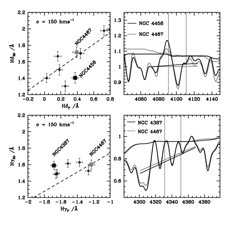
Figure 3: Comparison of the H$\gamma_{F}$ and H$\delta_{F}$ equivalent width measured with the side-band (SB) and the Boosted Median method (BMC). In order to eliminate the dependence of the EWs on velocity dispersion, we select those galaxies with $\sigma\leq 150$ km/s and smooth them to this maximum velocity dispersion. Top: We select NGC 4458 & NGC 4467, which show similar EWs in the SB method but have differing H$\delta$ EWs when using BMC. In the rightmost panels we plot the spectra from both galaxies. Overplotted are the pseudo-continuum of the side band (slanted straight line) and the BMC (running along the top of the SED). The identical EWs according to the SB method are due to the decreased flux in the red passband of NGC 4467, most likely caused by increased CN absorption, which hides the stronger intrinsic absorption in H$\delta$. The spectra are normalised to an average value of 1 across the blue passband of H$\delta_{F}$ to highlight the effect of CN absorption. Bottom: We highlight H$\gamma$ in NGC 4387 & NGC 4467, for which the SB method indicates a considerable difference in EW while the BMC identifies almost none. Looking at the spectra (right) of both galaxies we can see that the difference in EW from the SB method is caused by an increase in the depth of the G4300 feature, artificially lowering the pseudo-continuum. The spectra are normalised to 1 at 4365Å.

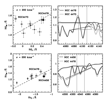
Figure 4: As in figure 3 we compare the H$\gamma_{F}$ and H$\delta_{F}$ equivalent widths measured with the side-band and the Boosted Median method. In order to eliminate the dependence of the EWs and spectra on velocity dispersion, we select – in contrast to figure 3 – those galaxies with $\sigma\leq 200$ km/s. The SEDs are smoothed to this maximum velocity dispersion. Top: The galaxies NGC 4473 & NGC 4478 are selected since they show differing H$\delta$ SB EWs but similar BMC measured EWs. The spectra (right) identifies the cause of the discrepancy. The spectra of NGC 4473 redwards of the H$\delta$ line is severely affected by CN absorption, lowering the average flux in this side band and distorting the derived pseudo-continuum. The BMC recovers a significantly more robust value. The spectra are normalised to an average value of 1 across the blue passband of H$\delta_{F}$ to highlight the effect of CN absorption. Bottom: NGC 4458 & NGC 4478 show discrepant SB EWs. This difference can be seen on the right, where the spectra of both galaxies are displayed. The BMC correctly identifies the larger value of H$\gamma$ in NGC 4478, which is hidden in the SB method due to the increased absorption of G4300 feature located in the blue pass band of H$\gamma_{F}$. The spectra are normalised to 1 at 4365Å.

Hence, the method for generating the BMC is fairly simple. At every wavelength the 90th percentile from all flux measurements within 50Å on either side is assigned as the continuum at that wavelength. With the continuum thus defined, for each line strength we only have to define the central wavelength and the spectral window over which the line is measured. Given that our method maps quite robustly the underlying continuum, we decided to fix a 20Å width for all line strengths considered in this paper – hereafter, our BMC-based equivalent widths are labelled with a $20$ subindex.

Table 2: Range of parameters explored in this paper (see text for a description of each model).

Model/Param	MIN	MAX	Comments
SSP			2 params
Age	3	13	Gyr
$\log(Z/Z_{\odot})$	-1.5	+0.3	Metallicity
EXP			3 params
$\log\tau$ (Gyr)	-1	+0.9	Exp. Timescale
$z_{F}$	0.1	5	Formation epoch
$\log(Z/Z_{\odot})$	-1.5	+0.3	Metallicity
2BST			4 params
tO	3	13	Old (Gyr)
tY	0.1	3	Young (Gyr)
fY	0.0	0.5	Mass fraction
$\log(Z/Z_{\odot})$	-1.5	+0.3	Metallicity
CXP			3 params
$\log\tau_{1}$ (Gyr)	-2	+0.5	SF Timescale
$\log\tau_{2}$ (Gyr)	-2	+0.5	Enrichment Timescale
$z_{F}$	0.1	5	Formation epoch

This is motivated by the fact that for some definitions of the line strengths, any ’contaminating’ lines falling within the central bandpass can have a stronger effect on the BMC method compared to the standard side-band method. A clear example is found in the $H\beta$ line, where the effect of FeI( 4871Å) which sits on the shoulder of the Balmer line within the standard definition of the central passband (width 28.75Å ) clearly distorts the measurement of the equivalent width. This is slightly ’compensated’ in the side-band method through the presence in the blue side-band of another significant Fe line at 4891Å. This is clearly not the case for the BMC method, in which the pseudo-continuum is effectively independent of the values of both Fe absortion lines. Hence, in the BMC method it is desirable to choose a central passband which only targets the line of interest. Nevertheless, the method is versatile enough to define wider central bandpasses.

Thus, to avoid this problem we define a central passband wavelength as narrow as possible within the usual spectral resolutions targeted in unresolved stellar populations. We follow the ’F’ type passbands as used for the Balmer indices (Worthey & Ottaviani, 1997), defining a 20Å window centered on the line of interest for all indices considered. In the case of the metal line strengths – which usually involve clusters of lines – the major feature is chosen as the center of the new 20Å  index. In the case of Mgb₂₀, this is centered between the MgI doublet at 5167/5172Å. Fe5270₂₀ is defined by the FeI line at 5270Å and Fe5335₂₀ uses the FeI line at 5328Å. The central passband of the G-band is 4300Å. Such a simple approach is nevertheless very versatile in its definition of any line strength. The new $D4000$ break feature uses the definition given by Balogh et al. (1999), with the difference that it is the ratio of the continuum flux obtained by the BMC method within those wavelengths that is used here.

Table 1 shows the (BMC-measured) equivalent widths of the Virgo elliptical galaxies targeted in this paper. The measurements are obtained directly from the observed spectra, presented in Yamada et al. (2006) and have not been corrected with respect to velocity dispersion. Analogously to the standard method, one could either correct the observed EWs for the effect of velocity dispersion, or use the observed EWs in the modelling. For the latter, one must then measure the model EWs on spectra with the same resolution and velocity dispersion as the targeted galaxy. We follow this approach in the paper. We note at this point that the effect of velocity dispersion on the EWs of Balmer lines measured with the BMC method is increased slightly since the method uses spectral information to better define the pseudo-continuum, which is destroyed by an increasing $\sigma$. This effect of course affects any other method which measures line strengths from unresolved spectra (e.g. Vazdekis & Arimoto, 1999). The numbers in brackets correspond to the 1-$\sigma$ uncertainty, obtained from a Monte Carlo simulation that generates 500 realizations of each SED, adding noise corresponding to the SNR of the observations. Notice that 6 of the galaxies do not have a measured D4000 as they were observed over a spectral range that does not include the blue passband used in the definition of D4000.

Table 3: Ages and metallicities of Virgo elliptical galaxies according to the four models used in this paper. Error bars quoted at the 90% confidence level.

Galaxy	SSP			2BST			EXP			CXP
NGC	Age(Gyr)	log(Z/Z⊙)	$\chi_{r}^{2}$	Age(Gyr)	log(Z/Z⊙)	$\chi_{r}^{2}$	Age(Gyr)	log(Z/Z⊙)	$\chi_{r}^{2}$	Age(Gyr)	log(Z/Z⊙)	$\chi_{r}^{2}$
4239	$5.0_{-0.6}^{+0.6}$	$-0.13_{-0.07}^{+0.07}$	0.29	$6.6_{-1.7}^{+2.6}$	$-0.14_{-0.08}^{+0.08}$	0.27	$5.3_{-0.8}^{+1.0}$	$-0.14_{-0.07}^{+0.07}$	0.27	$5.5_{-0.9}^{+0.6}$	$+0.06_{-0.07}^{+0.04}$	0.83
4339	$8.2_{-1.6}^{+1.6}$	$+0.18_{-0.10}^{+0.06}$	1.60	$8.5_{-1.9}^{+1.7}$	$+0.19_{-0.10}^{+0.06}$	1.58	$8.8_{-1.7}^{+1.5}$	$+0.16_{-0.09}^{+0.07}$	1.61	$9.6_{-1.7}^{+1.5}$	$+0.25_{-0.05}^{+0.03}$	1.23
4365	$11.6_{-0.6}^{+1.0}$	$+0.26_{-0.04}^{+0.03}$	2.30	$11.7_{-0.6}^{+0.9}$	$+0.26_{-0.04}^{+0.03}$	2.30	$11.4_{-0.4}^{+0.4}$	$+0.27_{-0.02}^{+0.02}$	2.76	$12.1_{-0.3}^{+0.1}$	$+0.30_{-0.02}^{-0.00}$	3.11
4387	$12.5_{-0.9}^{+0.4}$	$-0.09_{-0.05}^{+0.03}$	2.36	$12.4_{-1.1}^{+0.5}$	$-0.09_{-0.05}^{+0.03}$	2.36	$11.4_{-1.2}^{+0.5}$	$-0.06_{-0.03}^{+0.10}$	2.96	$11.4_{-0.9}^{+0.7}$	$+0.15_{-0.05}^{+0.02}$	3.15
4458	$10.7_{-0.8}^{+0.9}$	$-0.22_{-0.04}^{+0.04}$	4.34	$10.7_{-0.9}^{+1.0}$	$-0.22_{-0.04}^{+0.04}$	4.34	$10.7_{-0.7}^{+0.7}$	$-0.21_{-0.05}^{+0.04}$	5.06	$11.6_{-1.1}^{+0.8}$	$-0.01_{-0.07}^{+0.06}$	1.90
4464	$12.7_{-0.5}^{+0.2}$	$-0.14_{-0.03}^{+0.02}$	3.87	$12.7_{-0.4}^{+0.2}$	$-0.14_{-0.03}^{+0.02}$	3.87	$11.9_{-0.4}^{+0.2}$	$-0.13_{-0.02}^{+0.02}$	4.85	$12.0_{-0.6}^{+0.4}$	$+0.09_{-0.03}^{+0.01}$	3.68
4467	$6.4_{-1.1}^{+1.3}$	$+0.16_{-0.07}^{+0.06}$	2.79	$7.6_{-1.8}^{+2.6}$	$+0.19_{-0.07}^{+0.07}$	2.78	$6.8_{-1.3}^{+1.7}$	$+0.15_{-0.09}^{+0.06}$	3.33	$10.0_{-1.9}^{+1.8}$	$+0.21_{-0.06}^{+0.04}$	0.67
4472	$9.2_{-0.5}^{+0.6}$	$+0.27_{-0.02}^{+0.02}$	2.55	$9.4_{-0.5}^{+0.4}$	$+0.27_{-0.02}^{+0.02}$	2.55	$9.8_{-0.7}^{+0.8}$	$+0.27_{-0.02}^{+0.02}$	2.46	$11.3_{-0.8}^{+0.6}$	$+0.29_{-0.03}^{+0.00}$	2.19
4473	$12.5_{-0.8}^{+0.4}$	$+0.23_{-0.03}^{+0.05}$	1.65	$12.4_{-0.7}^{+0.5}$	$+0.23_{-0.03}^{+0.05}$	1.65	$11.6_{-0.5}^{+0.4}$	$+0.27_{-0.02}^{+0.02}$	2.59	$12.0_{-0.3}^{+0.1}$	$+0.30_{-0.02}^{-0.00}$	5.56
4478	$7.2_{-1.3}^{+1.3}$	$+0.22_{-0.07}^{+0.05}$	0.12	$7.6_{-1.6}^{+2.1}$	$+0.23_{-0.06}^{+0.04}$	0.12	$7.7_{-1.5}^{+1.6}$	$+0.21_{-0.07}^{+0.06}$	0.10	$8.6_{-1.3}^{+1.1}$	$+0.27_{-0.03}^{+0.02}$	0.03
4489	$4.6_{-0.8}^{+0.6}$	$+0.09_{-0.08}^{+0.08}$	2.82	$5.6_{-1.6}^{+2.3}$	$+0.10_{-0.09}^{+0.09}$	2.69	$5.0_{-0.9}^{+0.9}$	$+0.06_{-0.07}^{+0.09}$	2.84	$4.3_{-0.8}^{+0.5}$	$+0.25_{-0.05}^{+0.03}$	3.83
4551	$6.1_{-0.5}^{+1.0}$	$+0.26_{-0.04}^{+0.03}$	3.13	$10.0_{-2.0}^{+1.2}$	$+0.26_{-0.03}^{+0.02}$	2.50	$7.3_{-1.4}^{+2.1}$	$+0.26_{-0.05}^{+0.03}$	2.53	$9.8_{-2.2}^{+2.0}$	$+0.28_{-0.03}^{+0.01}$	2.29
4621	$10.5_{-0.3}^{+0.2}$	$+0.27_{-0.02}^{+0.02}$	10.73	$10.6_{-0.3}^{+0.3}$	$+0.27_{-0.02}^{+0.02}$	10.73	$10.9_{-0.2}^{+0.2}$	$+0.27_{-0.02}^{+0.02}$	10.67	$12.2_{-0.5}^{+0.2}$	$+0.30_{-0.02}^{-0.00}$	8.56
4697	$8.1_{-0.4}^{+0.6}$	$+0.27_{-0.02}^{+0.02}$	1.65	$8.1_{-0.5}^{+0.7}$	$+0.27_{-0.02}^{+0.02}$	1.65	$8.3_{-0.6}^{+1.0}$	$+0.26_{-0.04}^{+0.03}$	1.80	$11.0_{-1.3}^{+1.1}$	$+0.27_{-0.03}^{+0.01}$	0.24

3.2 Comparison with the side-band method

Figure  2 shows a comparison of the line strengths measured on the same spectra using the side-band (horizontal axes) and the BMC methods (vertical axes). Notice the departure from a simple linear relationship, mainly caused by the different way neighbouring lines affect the estimate of the pseudo-continuum. In figures 3 and 4 we illustrate in more detail the difference in the measurement of the equivalent width of H$\gamma$ and H$\delta$, looking more closely at the effect of nearby lines on the indices. In order to eliminate the dependence of the EWs on velocity dispersion we classify the sample into two subsets, according to velocity dispersion. Figure 3 considers only those galaxies with $\sigma\leq 150$ km/s and figure 4 focuses on galaxies with $\sigma\leq 200$ km/s. In both cases the galaxies are smoothed to the maximum velocity dispersion of the subsample, in order to make a consistent comparison. We note that by comparing spectra smoothed to some maximum $\sigma$ one would obtain a false sense of agreement between the methods, since the effect of smoothing removes information from the spectra.

The left panels of figures 3 and 4 compare the EWs of the galaxies in each subset (open black circles), but we focus on two galaxies in each case (solid squares). The galaxies are chosen because they have a similar value of the EW using one method, and a significantly different value using the other method. The spectral regions targeted in those galaxies is shown in the rightmost panels. The straight short line intersecting the spectra is the side-band pseudo-continuum and runs between the centres of the flanking side band regions The continuous line running along the top of the spectra is the BMC continuum. These are shown in grey and black for each galaxy, as labelled. The spectra are normalised to allow us to overplot both SEDs. In the case of H$\gamma$ we follow  Vazdekis & Arimoto (1999) and normalise at the peak of 4365Å. For H$\delta$ we normalise to an average flux value of 1 within the wavelengths of the blue side-band, to highlight the effect of CN absorption towards the red side of the line.

In figure 3 we show those galaxies with $\sigma\leq 150$ km/s. In the top panels, we focus on NGC 4458 and NGC 4467, since these galaxies give a similar side-band H$\delta$ EW but very different BMC-based measurements. Looking in detail at the SEDs on the right, the red side-band of NGC4467 is more affected by increased absorption, mainly caused by the CN features which, as reported in Yamada et al. (2006), are stronger in NGC4467 (CN₁=0.110 mag), than in NGC4458 (CN₁=0.074 mag). Notice that this does not strongly affect the BMC pseudo-continuum. In addition, the H$\delta$ absorption observed in NGC 4467 is possibly underestimated relative to NGC 4458. The iron abundance reported by Yamada et al. (2006) is higher in NGC 4467 by $\sim$0.1 dex, an effect that would be hidden by the normalisation over the iron lines around $\sim$4070Å. In the bottom panels of figure 3 we investigate the H$\gamma$ lines in NGC 4387 and NGC 4467 which have a similar EW using the BMC method, whereas they differ by $\sim$0.5 Å in the side-band method. The SEDs reveal that these two galaxies do indeed have similar Balmer absorption, but the side-band method is ’tricked’ when comparing the flux with the continuum (straight line). The increased G4300 absorption in NGC 4387 pushes the pseudo-continuum down, which reduces the EW value incorrectly. This is consistent with the measured absorption at this resolution of NGC4467 (G4300₂₀ = 6.5 Å) compared to that in NGC4387 (G4300₂₀ = 7.2 Å).

Shown in figure 4 is the subsample with higher velocity dispersion, comparing galaxies at $\sigma\leq 200$km/s. The top panel shows the considerable discrepancy between the side band and BMC methods on measuring H$\delta$. Since the over-abundance of CN and the resulting absorption tends to increase with the mass of the galaxy (see e.g. Sánchez-Blázquez et al., 2003; Toloba et al., 2009), the inclusion of the more massive NGC 4473 serves to show how significant the effect can be. The $\sim$0.6Å  difference in H$\delta$ given by the side band method can be seen to be generated by the increase in absorption in the red side-band region $\sim$4120Å, of NGC4473. We note again that the CN absorption, identified by Yamada et al. (2006) is higher in NGC 4473 (CN₁=0.138 mag), than in NGC 4478 (CN₁=0.077 mag). The bottom panels display a more subtle situation in which the effect of the surrounding metal lines is to reverse the relative values of the H$\gamma$ EWs. The increased absorption, again mainly coming from the G4300 feature, forces the pseudo-continuum to a lower value, resulting in a small EW. The effect, while small, serves to indicate how sensitive the side band method can be to the surrounding spectral features.

Therefore, figures 3 and 4 show that our proposed method is more resilient to the effects of neighbouring absorption lines. To further illustrate this point, figure 5 compares the age-metallicity degeneracy of typical Balmer (left) and metal lines (right) measured either in the standard way or using the BMC pseudo-continuum. The shaded areas indicate the difference in the EWs with respect to a reference stellar population: on the left it is the population with the same age at solar metallicity, and on the right the reference is a population with the same metallicity and 10 Gyr old, both references marked by the vertical lines. Black and grey shading correspond to the BMC and the side-band methods, respectively. The panels on the left explore the age-sensitive Balmer indices for a range of metallicities and the panels on the right show metal indices for a range of ages. Ideally, a perfect observable would result in a horizontal line (i.e. zero metallicity dependence of an age-sensitive line and vice-versa). The models span a wide range of ages and metallicities as shown in the caption. This figure shows that BMC-based measurements of EWs are less subject to the age-metallicity degeneracy than the side-band methods. This result is especially dramatic for H$\gamma$ and H$\delta$, for which the age-metallicity degeneracy drops from $\Delta$EW$/\Delta\log(Z/Z_{\odot})=-4.2$ (side-band) to $-1.9$ (BMC) in H$\gamma$ or from $-3.9$ (side-band) to $-1.7$ (BMC) in H$\delta$ (values measured at the fiducial 10 Gyr, solar metallicity SSP). Furthermore, the shaded regions of the metal-line indices on the rightmost panels are much wider for the BMC method (black), showing that at a fixed age, the BMC method spans a wider range of EW, thereby being more sensitive to metallicity (see caption for details).

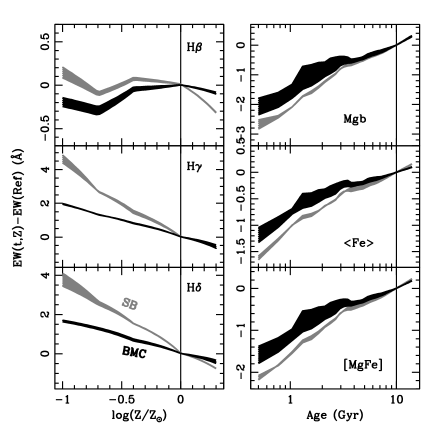
Figure 5: Dependence of Balmer lines on metallicity (left) and “metal” lines on age (right). The standard side-band method (SB; grey) and our proposed Boosted Median Continuum (BMC; black) are shown for a range of metallicities and ages as shown. On the left, the shaded areas correspond to an age range $[6,12]$ Gyr. On the right, the shaded areas span a range of metallicities: $-0.3<\log Z/Z_{\odot}<+0.3$. The vertical axis is the difference between the equivalent width of the line for a given metallicity (left) or age (right) and the value at a reference point given by the vertical line (i.e. solar metallicity on the left and 10 Gyr on the right).

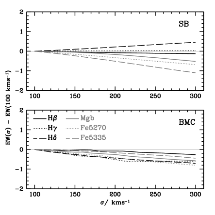
Figure 6: The uncertainties caused by an error in the estimate of velocity dispersion are illustrated by a comparison of the difference between the EW measured at a fiducial value ($\sigma=$100km/s) and a range of velocity dispersions (horizontal axis). Various line strengths are considered, as labelled, for the standard SB method (top) and our proposed BMC method (bottom).

In order to quantify the effect of an uncertainty in the velocity dispersion on the EWs, we compare in figure 6 the change in EW between a fiducial value ($\sigma=$100km/s) and a range of velocity dispersions (horizontal axis). The SB (BMC) values are shown in the top (bottom) panels for a number of absorption lines, as labelled. One can see that the effect on BMC-measured EWs can be corrected much in the same as with the standard SB method. In addition, for most cases the correction is smaller for BMC estimates.

Furthermore, we have compared the effect of noise on our proposed BMC pseudo-continuum and found that for a wide range of signal-to-noise ratios (from 10 to 100 per Å ) the uncertainty in the EW of all lines is always $\sim 0.3$ dex smaller than those obtained with the side-band method. However due to the lower dynamical range, as the BMC is forced to stay above the spectra, the S/N requirements are similar to other methods. We follow Cervantes & Vazdekis (2009) and define the S/N at which the method can distinguish $\pm$2.5 Gyr at 10 Gyr. For $H\gamma$ and $H\delta$ we get a S/N of $\sim 50$, and for $H\beta$ the required S/N is $\sim 60$.

Figure 7 shows the equivalent widths of several lines for a grid of SSPs corresponding to a velocity dispersion of 100 km/s (black) or 300 km/s (grey). The measured EWs (without any correction for velocity dispersion) are shown as black dots, along with a characteristic error bar which mostly comes from the systematics (the observed uncertainties are much smaller). We emphasize that our fitting method generates grids corresponding to the measured velocity dispersion for each galaxy. One can see that BMC EWs (left panels) appear less degenerate than the grids using a side-band method (right panels).

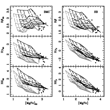
Figure 7: Comparison of grids of SSP models using the standard side-band method (SB, right) and our proposed Boosted Median Continuum (BMC, left). A systematic error bar is included in each panel (the observational error bars are much smaller). We show the grids for two different velocity dispersions 100km/s (black) and 300km/s (grey). The solid lines connect the SSPs with ages (from top to bottom) 2 to 14 Gyr in steps of 2 Gyr. The dashed lines connect the SSPs with metallicities (from left to right) [m/H]=$-$1 to $+$0.2 in steps of 0.2 dex.

4 Modelling the SFH of elliptical galaxies

The properties of the unresolved stellar populations of our sample are constrained by comparing the targeted equivalent widths with four sets of generic models that describe the star formation history in terms of a reduced number of parameters. It is our goal to assess the consistency of different sets of models in fitting independently the different spectral lines targeted as well as the full SED. The majority of studies in the literature (see e.g. Kuntschner & Davies, 1998; Trager et al., 2000; Caldwell et al., 2003; Thomas et al., 2005) have compared measurements of EWs with simple stellar populations (i.e. a single age and metallicity). While those models are probably valid for the populations found in globular clusters, it is imperative to go beyond simple stellar populations in galaxies, whose star formation histories generate complex distributions of age and metallicity. Ferreras & Yi (2004) and Pasquali et al. (2003) showed that composite models of stellar populations could result in significant differences on the average ages and metallicities of galaxies. More recently, Sánchez-Blázquez et al. (2006) and Serra & Trager (2007) have explored this issue through the comparison of two age indicators, both concluding that composite populations are needed to consistently model the populations in early-type galaxies.

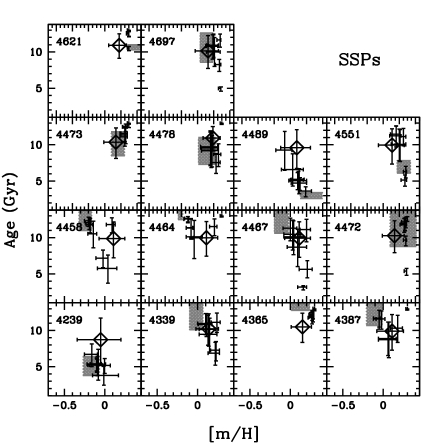
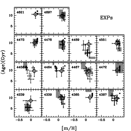
Figure 8: Best fit age and metallicity values for our sample, using SSPs (left) or EXP models (right). The error bars shown the 68% confidence levels and the shaded regions give the age and metallicity estimates of Yamada et al. (2006) using the H$\gamma_{\sigma}$ vs. [MgFe] diagram. The diamond gives the fit to the age and metallicity using only the spectral energy distribution (i.e. no line strengths are used for this data point).

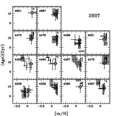
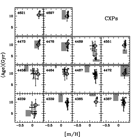
Figure 9: Best fit age and metallicity values for our sample, using 2-Burst (left) or CXP models (right). The error bars shown the 68% confidence levels and the shaded regions give the age and metallicity estimates of Yamada et al. (2006) using the H$\gamma_{\sigma}$ vs. [MgFe] diagram. The diamond gives the fit to the age and metallicity using only the spectral energy distribution (i.e. no line strengths are used for this data point).

In this paper, except for the first case (namely Simple Stellar Populations), the models generate a distribution of ages and/or metallicities that are used to combine the population synthesis models of Bruzual & Charlot (2003), assuming a Chabrier (2003) Initial Mass Function. We use the updated 2007 version (Bruzual, 2007). The resulting synthetic spectral energy distribution is smoothed to the same resolution and velocity dispersion of the galaxy. A correction for Galactic reddening is applied, assuming the Fitzpatrick (1999) law (this is mostly done for the comparison of the full SEDs, as EWs are not affected). Finally, the EWs are computed and compared with the observations using a standard maximum likelihood method. The high S/N of the observed spectra imply that our error budget is mainly dominated by the systematics of the population synthesis models. It is not obvious how to incorporate problems such as sparsely populated stellar parameter space or systematics within the models, into the analysis. As a compromise we estimate the uncertainties associated with the models by generating 500 Monte Carlo simulations of gaussian noise at the level of S/N $\sim$50, that of the stellar library at the core of the BC03/CB07 models (STELIB Le Borgne et al., 2003). These are added in quadrature with those generated for each galaxy index.

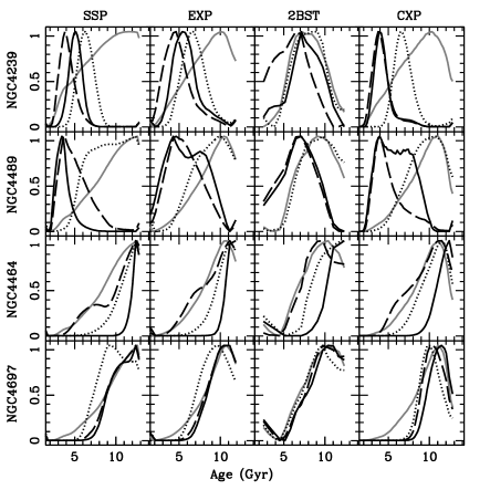
Figure 10: Likelihood distribution of the marginalised average stellar ages for some of the Virgo cluster elliptical galaxies from our sample. The distribution is shown for the four models as labelled. The grey solid line corresponds to the fit of the SED. The lines correspond to the age distribution according to [MgFe] plus either H$\beta$ (black,solid), H$\gamma$ (black,dashed) or H$\delta$ (black,dotted), respectively.

The four sets of models considered in this paper are listed below, with the range of parameters shown in table 2.

1. Simple Stellar Populations (SSP): This has been the most popular method used in the analysis of the ages and metallicities of early-type galaxies. The advantage lies in it simplicity: SSPs are the building blocks of all population synthesis models, and they are carefully calibrated against realistic SSPs (i.e. globular clusters). An SSP is primarily defined by an age and a metallicity although it is also dependent on the abundance pattern and the IMF. The drawback of this method is that the parameters obtained are inherently luminosity weighted, such that a small amount of young stars can have a significant effect on the age extracted with this method. Furthermore, SSPs are not expected to model galaxy populations, which have an extended range of ages and metallicities. By using SSPs to model early-type galaxies one makes the assumption that the stellar populations have a narrow age distribution compared to stellar evolution timescales.

2. Exponential SFH (EXP): A more physical scenario should consider an extended period of star formation. The EXP models (also called $\tau$ models in the literature) model the star formation rate as an exponentially decaying function of time with timescale $\tau$, started at an epoch given by a formation redshift $z_{F}$. The metallicity is assumed to be fixed throughout the SFH and is also left as a free parameter.

3. Two Burst Formation (2BST): Recent rest-frame NUV observations have revealed the presence of residual star formation in early-type galaxies (see e.g. Trager et al., 2000; Ferreras & Silk, 2000; Yi et al., 2005; Kaviraj et al., 2007). The presence of small amounts of young stars can significantly affect the derived SSP model parameters (Serra & Trager, 2007). This model describes this mechanism with two simple stellar populations. Four parameters are left free: the age of the old (t_O) and the young components (t_Y), the mass fraction in young stars (f_Y), and the metallicity of the populations ($Z$, assumed to be the same for the old and the young components).

4. Chemically Enriched Exponential (CXP): All the models considered above fix the metallicity throughout the SFH. More realistically, a model should incorporate in a consistent way the buildup of metallicity caused by previous generations of stars. These chemical enrichment models (see e.g. Boissier & Prantzos, 1999; Ferreras & Silk, 2003) include the stellar yields from intermediate and massive stars and result in a distribution of metallicities as well as ages. The aim of this paper is to explore simple models that can be easily implemented. Hence, instead of applying a detailed model of chemical enrichment, we define in a purely phenomenological way a model that mimics those. We keep the same SFH as in the EXP models (described by a star formation timescale $\tau_{1}$ and a formation redshift $z_{F}$). Furthermore, the metallicity is assumed to increase in step with the cumulative distribution of the star formation rate, namely:

   $$Z(t)=Z_{1}+(Z_{2}-Z_{1})\Big{[}1-\exp(-\Delta t/\tau_{2})\Big{]},$$ (2)

   where $\Delta t=t-t(z_{F})$ and $\tau_{2}$ is the timescale corresponding to the buildup of metallicity. As a first-order approach it is valid to assume that metallicity increases with the stellar mass of the system (roughly, the cumulative distribution of the star formation rate). More accurately, this timescale will depend on the star formation efficiency or on the fraction of gas ejected in outflows (see e.g. Ferreras & Silk, 2003). The upper and lower values of metallicity are fixed to $Z_{1}=Z_{\odot}/10$ and $Z_{2}=2Z_{\odot}$, although the average metallicity will be controlled by the timescale $\tau_{2}$.

Figure 11: Comparison between the ages presented here and those from previous studies. Y06, TF02 and C03 indicate (Yamada et al., 2006), (Terlevich & Forbes, 2002), and (Caldwell et al., 2003), respectively. The figure illustrates the difference in the average ages when including two types of composite populations: a 2-burst model (2BST; top) or a smooth star formation history including chemical enrichment (CXP; bottom). The slanted solid line is a 1:1 correspondence. The vertical dashed line represents the age of the Universe for our cosmology, and is used as a prior in the analysis (see text for details).

We assume a standard $\Lambda$CDM cosmology ($\Omega_{m}$=0.3; H₀= 70 km/s/Mpc) to constrain the maximum ages of the stellar populations to the age of the Universe (13.7 Gyr). One could allow the fitting algorithm to stray into older ages to explore wider volumes of parameter space, but this paper takes the cosmological constraints on the age of the Universe at face value (Spergel et al., 2007). Furthermore, population synthesis models are poorly calibrated for populations older than Galactic globular clusters. We note that previous work on the same spectra (Yamada et al., 2006) probed the population synthesis models of Vazdekis & Arimoto (1999) all the way to their oldest available ages ($\sim$20 Gyr), using the isochrones of Bertelli et al. (1994). Although in only two cases, NGC4365 at 20 Gyr and NGC4464 at 18.5 Gyr, did they find cosmologically contradictory ages, we still choose to avoid this by limiting the maximum age.

Table 4: Best fit parameters for the 2BST and CXP models

Galaxy	M${}_{\rm s}^{1}$	2BST			CXP
NGC	$\times 10^{10}$M⊙	tO(Gyr)	tY(Gyr)	fY	$\tau_{1}$(Gyr)	$\tau_{2}$(Gyr)	zF
4239	0.9(0.7)	$7.9_{-2.7}^{+2.7}$	$2.6_{-0.3}^{+0.3}$	$0.08_{-0.06}^{+0.12}$	$0.2_{-0.2}^{+0.5}$	$0.2_{-0.1}^{+0.5}$	$0.6_{-0.1}^{+0.2}$
4339	4.6(4.6)	$8.8_{-2.0}^{+1.8}$	$1.8_{-1.3}^{+1.1}$	$\lower 2.15277pt\hbox{$\;\buildrel<\over{\sim}\;$}0.01$	$0.4_{-0.2}^{+0.4}$	$0.0_{-0.0}^{+0.1}$	$1.7_{-0.5}^{+0.8}$
4365	38.0(36.3)	$11.9_{-0.9}^{+0.7}$	$1.5_{-1.1}^{+1.0}$	$\lower 2.15277pt\hbox{$\;\buildrel<\over{\sim}\;$}0.01$	$0.8_{-0.2}^{+0.2}$	$2.9_{-2.0}^{+2.0}$	$3.0_{-0.2}^{+0.2}$
4387	3.2(2.8)	$12.4_{-0.8}^{+0.5}$	$1.6_{-1.1}^{+1.0}$	$\lower 2.15277pt\hbox{$\;\buildrel<\over{\sim}\;$}0.01$	$0.7_{-0.3}^{+0.4}$	$0.3_{-0.1}^{+0.2}$	$2.6_{-0.5}^{+0.5}$
4458	3.1(2.2)	$10.9_{-1.0}^{+0.7}$	$1.6_{-1.1}^{+1.0}$	$\lower 2.15277pt\hbox{$\;\buildrel<\over{\sim}\;$}0.02$	$0.2_{-0.1}^{+0.4}$	$0.2_{-0.2}^{+0.6}$	$2.5_{-0.4}^{+0.6}$
4464	1.8(1.4)	$12.7_{-0.5}^{+0.2}$	$1.6_{-1.1}^{+1.0}$	$\lower 2.15277pt\hbox{$\;\buildrel<\over{\sim}\;$}0.01$	$0.6_{-0.2}^{+0.3}$	$0.4_{-0.2}^{+0.2}$	$2.8_{-0.4}^{+0.3}$
4467	0.4(0.4)	$8.6_{-2.6}^{+2.6}$	$2.4_{-1.1}^{+0.5}$	$0.03_{-0.03}^{+0.11}$	$0.2_{-0.1}^{+0.1}$	$0.1_{-0.1}^{+0.1}$	$1.7_{-0.6}^{+0.8}$
4472	97.7(102.3)	$9.5_{-0.8}^{+0.4}$	$1.6_{-1.1}^{+1.0}$	$\lower 2.15277pt\hbox{$\;\buildrel<\over{\sim}\;$}0.02$	$0.9_{-0.4}^{+0.6}$	$0.2_{-0.2}^{+0.2}$	$2.8_{-0.4}^{+0.3}$
4473	20.4(20.4)	$12.5_{-0.8}^{+0.4}$	$1.5_{-1.1}^{+1.0}$	$\lower 2.15277pt\hbox{$\;\buildrel<\over{\sim}\;$}0.01$	$1.0_{-0.1}^{+0.2}$	$1.6_{-1.1}^{+1.1}$	$3.0_{-0.2}^{+0.2}$
4478	4.7(5.6)	$8.3_{-2.2}^{+2.1}$	$1.9_{-1.3}^{+1.0}$	$0.02_{-0.02}^{+0.05}$	$0.6_{-0.3}^{+0.5}$	$0.1_{-0.1}^{+0.1}$	$1.4_{-0.3}^{+0.6}$
4489	1.2(1.2)	$6.9_{-2.5}^{+2.4}$	$2.6_{-0.4}^{+0.3}$	$0.13_{-0.10}^{+0.18}$	$0.3_{-0.1}^{+0.3}$	$0.1_{-0.1}^{+0.1}$	$0.4_{-0.1}^{+0.1}$
4551	4.0(2.8)	$10.7_{-2.0}^{+1.7}$	$2.7_{-0.2}^{+0.2}$	$0.04_{-0.03}^{+0.06}$	$0.3_{-0.1}^{+1.1}$	$0.2_{-0.1}^{+0.1}$	$1.7_{-0.6}^{+0.9}$
4621	33.9(33.1)	$10.7_{-0.4}^{+0.1}$	$1.5_{-1.1}^{+1.0}$	$\lower 2.15277pt\hbox{$\;\buildrel<\over{\sim}\;$}0.02$	$1.0_{-0.3}^{+0.3}$	$1.4_{-1.0}^{+1.0}$	$4.1_{-1.2}^{+0.9}$
4697	17.0(12.3)	$8.3_{-0.7}^{+0.4}$	$1.6_{-1.2}^{+1.0}$	$\lower 2.15277pt\hbox{$\;\buildrel<\over{\sim}\;$}0.03$	$0.3_{-0.1}^{+0.4}$	$0.2_{-0.1}^{+0.1}$	$2.3_{-0.4}^{+0.5}$

¹ Stellar masses are computed from the best fit CXP (2BST) models. Estimated uncertainty $\Delta\log$M${}_{s}\sim 0.3$ dex (mostly from the assumption about the IMF).

4.1 Disentangling the stellar populations

The comparison of the EWs is done by measuring the line strengths directly from the model SEDs after being resampled and smoothed to the resolution and velocity dispersion of the actual observations of each galaxy, taken from Yamada et al. (2006). Since the spectra of the models have already been smoothed in terms of velocity dispersion to that of the real galaxy, no correction for this need be applied. All galaxies are fitted using the age-sensitive indices, H$\beta_{20}$, H$\gamma_{20}$, H$\delta_{20}$ and G4300₂₀ along with the metallicity indicator [MgFe]₂₀(González, 1993). This is used instead of the newer [MgFe]^′ as defined by Thomas et al. (2003) since the original is almost independent of $\alpha/$Fe and it is not clear whether the same fractions of the two Fe lines is still appropriate for the new BMC indices. We note that we have excluded the D4000 index since it was found to be poorly modelled by BC03, a problem already identified by both Wild et al. (2007) and Sánchez-Blázquez et al. (2006c). The exclusion (or inclusion) of the D4000, does not significantly affect the final results obtained although it does significantly increase (decrease) the quality of the fit. The removal of the D4000 also limits the constraints we can put on second order parameters (e.g. age and mass fraction of young stellar population in the 2-Burst model).

As indicated by Schiavon et al. (2004) and later confirmed by Serra & Trager (2007), a discrepancy found between the parameters derived through each of the three Balmer lines could be explained by the existence of an underlying younger sub-population. Schiavon et al. (2004) explain that this may well be due to the dominance of the younger population at bluer wavelengths. However the mere fact that different indices would give different parameters, should suggest that the model being used has not captured all aspects of the true star formation history. Hence, in the analysis of EWs of our sample galaxies, we are not only looking to determine the age and metallicity but also estimating whether it is possible to rule out a single population to describe an early-type galaxy. This could be done through discrepancies between the three Balmer lines targeted here, a possibility highlighted by Schiavon et al. (2007) on a single stacked spectra of low mass ellipticals, who found that the addition of a small young population alleviated such discrepancies.

With the same aim, we focus on possible discrepancies between individual line strengths and explore a number of star formation histories to determine the age distribution of our sample of elliptical galaxies.

4.2 Spectral Fitting

As an alternative approach to targeted line strengths, we also consider the full spectral energy distribution to constrain the star formation history of our sample. In this paper we want to test the consistency between the constraints imposed by the line strengths and those from a full spectral fit.

We use a maximum likelihood method to fit the spectra, which is analysed over the spectral range between 3900Å and 4500Å (or 4000–4500Å for the six galaxies observed with WHT). The SEDs are normalised over the same range. The data span a much wider spectral range (out to 5500-5800Å). However, we have chosen a smaller range to avoid flux calibration errors, which could introduce important systematic changes in the predicted ages and metallicities. The spectral range chosen straddles the D4000 break, since this is a very sensitive indicator of the ages of the stellar populations.

4.3 Results

Figures 8 and 9 show the average age and metallicity for all four models explored in this paper. The error bars are shown at the 69% confidence level (i.e. like a 1$\sigma$ level although our analysis does not assume a Gaussian distribution). For the SSPs the average age is trivially the age of the population. For the others, the average values are weighed by the stellar mass. Each error bar corresponds to the individual fit of an age-sensitive line (H$\beta$, H$\gamma$, H$\delta$ or G4300) plus the [MgFe] as metallicity indicator (i.e. each point comes from the analysis involving 2 indices). The diamond and its error bar correspond to the fit to the SED – no additional information from the line strengths is added to this likelihood. In grey, the shaded areas correspond to the ages from Yamada et al. (2006) (using the H$\gamma_{\sigma}$ – [MgFe] diagram on SSPs). One can see that SSPs (left panel of figure 8) show the largest discrepancies between the ages and metallicities estimated using independently the different age-sensitive indices. This would imply that a joint likelihood putting all indices together would not be a consistent way of determining the ages of the populations.

Nevertheless, as a comparison we show in table 3 the best estimates of the average age and metallicity, combining all five indices (but not the fit of the SED). Table 4 shows the best fit parameters for the 2BST and CXP models. The uncertaintes in both tables are given at the 90% confidence level. It can be seen from table 3 that in a majority of cases the use of a model with an age spread offers an improvement in the $\chi^{2}$ value for the five indices. Importantly the recovered values of metallicity remain consistent (within errors) across the single metallicity models considered, indicating its robustness against the inclusion of additional populations. For some galaxies, such as NGC 4365, NGC 4387 and NGC 4473, an SSP is as good as the other models presented here and in fact the parameters recovered by complex SFHs essentially reduce to an SSP. This is to be expected since the short formation timescale expected for elliptical galaxies will in some cases be well represented by an SSP. However galaxies which have younger SSP ages give very different (mass-weighted) ages when considering a 2-Burst model. One interesting result is that the CXP models, which incorporate a spread both in metallicity and age, find solutions that are as good as – and in the case of NGC4458, and NGC4467 and NGC 4697 significantly better than – the other models.

In addition, the discrepancies among individual measurements shown in figure 8 reflects the fact that a single age and metallicity scenario is a weaker, less consistent model of the populations of a galaxy. Table 3 shows that the actual change in the age when going beyond SSPs can be quite significant, especially for younger ages. We emphasize here that the different ages do not reflect a possible inclusion of a prior caused by the choice of parameters. All the composite models presented here (CSP, EXP and 2-Burst) explore a range of parameters that includes the best-fit ages and metallicities obtained by the SSPs.

In some cases the $\chi^{2}$ values are larger than might be expected. In the case of NGC 4621, the largest contributor is the G-band. If we remove that indicator from the analysis, the reduced $\chi^{2}$ decreases to $\sim 1$. It is clear that the high S/N of the spectra poses a challenge for current stellar population synthesis models. Certainly the errors associated with the models do not take into consideration internal problems with the models themselves or the possible limitations of the stellar libraries from which they are assembled. Proctor et al. et al. (2004) also consider that limitations in the models as the cause of the high $\chi^{2}$ values.

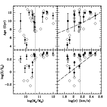
Figure 12: Ages and metallicities versus stellar mass (left) and velocity dispersion (right). The solid dots (grey diamonds) correspond to the estimates from the CXP (2-Burst) models. The dashed lines in the rightmost panels are the age and metallicity scaling relation of Thomas et al. (2005).

The mismatch discussed above can be seen in more detail in figure 10, where the marginalised distribution of average age for all four models is shown for a few galaxies from the sample, as labelled. The black solid, dashed, and dotted lines correspond to individual fits to H$\beta$, H$\gamma$, and H$\delta$, respectively, along with the G4300 (grey, dotted) and the SED (grey, solid). SSPs (leftmost panels) fail to give a consistent distribution, whereas any of the other models give a more unified distribution. Notice that the galaxies shown in the top panels (NGC 4239 and NGC 4489) have young populations, whereas the bottom two galaxies (NGC 4464 and NGC4697) have overall older populations. The top two galaxies are better fit by a 2-Burst model and the bottom two get better fits from an extended model like CXP. This would suggest that the youngest populations in early-type galaxies are best fit by the assumption of “sprinkles” of young stars, as suggested by Trager et al. (2000) and modelled by Ferreras & Silk (2000) and Kaviraj et al. (2007).

This explains why the models incorporating an age spread have greater maximum likelihood values, where $\mathcal{L}_{max}\propto\exp(-\chi^{2}_{min}/2)$. However, as was seen in table 3, the fits of the SSPs are not substantially worse than the more complex models. This is not surprising given firstly, that the SFH of many elliptical galaxies is not different from a single episode of star formation, especially when it happens at high redshift. Secondly, as identified by Serra & Trager (2007), for bursts of mass fraction, $f_{\rm Y}\geq$ 10% the disagreement in the recovered ages from different Balmer lines dissappears. This indicates that there is no differential effect across the spectrum from which to determine an age spread. Nevertheless, it remains the case that the more complex models are physically well motivated, resulting in better average age estimates and fit the data more consistently. Under such criteria we select the 2BST and CXP for further analysis.

Figure 11 shows a comparison of our age estimates using 2-Burst (top) and CXP models (bottom) with values taken from the literature, as given in the figure caption. It is important to notice that our models do not consider ages older than the age of the Universe using a concordance $\Lambda$CDM cosmology (i.e. 13.7 Gyr). Our ages are also closer to a mass weighted average due to the underlying assumptions in the modelling in both cases. We find that for the youngest galaxies, our analysis gives rather older ages than previous estimates from the literature. Also notice that the older galaxies appear younger because of the strong constraint imposed by the chosen cosmological parameters. Figure 12 shows the average age and metallicity as a function of stellar mass ( left) and velocity dispersion (right), both for the CXP (black dots) and for the 2-Burst models (grey diamonds). The stellar masses are obtained by combining the absolute magnitude of the galaxies in the $V$ band with $M/L_{V}$ corresponding to the best fit CXP models (There is no significant difference if the best fit 2-Burst models are used instead). The dashed line is the fit to age and metallicity from Thomas et al. (2005). Our age-mass relationship is compatible with recent estimates in the literature (see e.g. Trager et al., 2000; Caldwell et al., 2003; Thomas et al., 2005; Sánchez-Blázquez et al., 2006b). We should emphasize that our reduced sample of Virgo elliptical galaxies excludes massive, young S0s in high density environments (Thomas et al., 2005), removing them as a possible cause of the age scatter.

Figure 13: The predictions of the CXP models for star formation timescale ( top) and formation redshift (bottom) are shown with respect to stellar mass (left) and velocity dispersion (right). This speculative plot suggests that the age trend found in figure 12 is mainly caused by a range of formation epochs (bottom). The formation timescale (top) also correlates with mass or velocity dispersion, but it does not have values larger than $\tau_{1}\sim 1.5$ Guyr. The solid lines in the right panels are simple linear fits to the data (equations 3 & 4, see text for details).

Furthermore, notice in figure 12 the transition in the age distribution around 150 km/s in velocity dispersion or 5$\times$10${}^{10}M_{\odot}$ in stellar mass. Above this value the ages of the populations are overall old and with small scatter among galaxies, whereas lower mass galaxies have a wide range of ages and metallicities (not necessarily younger throughout). The trend is robustly independent of the modelling, as shown both by the CXP fits (black dots) and the 2-Burst models (grey diamonds). This threshold is reminiscent of the one found by Kauffmann et al. (2003) in the general population of SDSS galaxies at a stellar mass $3\times 10^{10}M_{\odot}$ or the threshold in star formation efficiency of late-type galaxies at rotation velocities v${}_{c}\sim$140 km/s based on their photometry (Ferreras et al., 2004) or on the presence of dust lanes (Dalcanton et al., 2004).

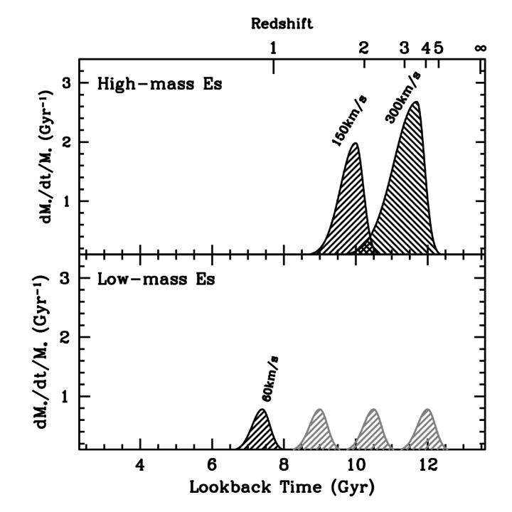
Figure 14: Our proposed model for the star formation history of Virgo cluster elliptical galaxies. The parameter estimates suggest a nearly constant star formation timescale with respect to velocity dispersion, whereas formation epoch is strongly correlated. We find a stronger correlation with velocity dispersion (compared to stellar mass), so we label the formation scenarios according to $\sigma$. The bottom panel emphasizes the issue that the observed low-mass Es are best fit by later formation epochs, an issue which does not rule out the possibility of other low-mass Es in the past – or elsewhere – to have been formed earlier (grey Gaussians).

5 Conclusions

We have revisited the superb, high signal-to-noise spectra of 14 elliptical galaxies in the Virgo cluster presented by Yamada et al. (2006, 2008). Our main goal was two-fold: a) to give an optimal but versatile definition of the equivalent width of spectral features that would minimise the contribution from nearby lines, b) to explore the possibility of discriminating between the standard treatment of galaxy spectra either as simple stellar populations or composite models with a distribution of ages and metallicities.

The former was achieved by defining a “boosted median” pseudo-continuum. This method is very easy to implement on any spectral data and it improves on the traditional side-band methods by reducing the final uncertainty of the EWs for the same spectra and reducing the age-metallicity degeneracy of age- and metal-sensitive lines by reducing the effect of unwanted, nearby spectral features. The method only requires two numbers to determine the pseudo-continuum (i.e. confidence level of the boosted median and size of the kernel over which the analysis is performed). We propose 90% and 100Å for these two parameters when dealing with stellar populations of galaxies at moderate resolution (R$\sim 1000-2000$).

The second goal – going beyond SSPs – is approached by comparing SSPs and three more sets of models which assume some distribution of ages and metallicities. We find simple populations fail to give a consistent marginalised distribution of ages when fitting independently different age-sensitive lines. We propose either a 2-Burst model or a $\tau$ star formatiom history with a phenomenological prescription for chemical enrichment (CSP models). They give similar results, with a clear trend between average age and either stellar mass or velocity dispersion, as shown in figure 12.

As suggested above when discussing figure 10, if younger (older) galaxies are better fit by 2-Burst (CXP) models, one would expect that young stars in elliptical galaxies appear in a random way, and not as a time-coherent, smooth distribution. This result supports minor merging – possibly involving metal-poor sub-systems – as the main mechanism to generate recent star formation in early-type galaxies (Kaviraj et al., 2009). This process will be readily detected in low-mass galaxies, whereas a similar amount of young stars in a massive galaxy will be harder to detect.

Doubtlessly average ages and metallicities are the observables best constrained by these models. Parameters like formation timescale and formation epoch can only be considered “next-order” observables, which will be fraught with larger uncertainties. This is largely due to the massive degeneracies which are present in such parameters as mentioned in the introduction. Its is well known that the mass and age of a subpopulation are degenerate in that additional mass fraction can compensate for an older age or vice versa (Leonardi & Rose, 1996). Another considerable degeneracy also exists between the formation redshift and the star formation timescale for both the EXP and CXP models (see e.g. Gobat et al., 2008). While our indices cover a large wavelength range we find that these degeneracies are still significant. Figure 15 shows the degeneracy between parameters for a typical case using 2-Burst models (left) and CXP models (right). We take the probability weighted values across the entire parameter space as a more robust measure of these parameters. Although the derived parameters are still subject to considerable uncertainty, as expressed by the error bars shown in figure 13, we note that our grids sample the parameter space quite finely meaning our recovered likelihood distribution should be a reasonable approximation to the complete distribution.

We proceed in a more speculative way, taking the continuous CXP models at face value and putting some trust on the predictions of their formation epochs and timescales. Figure 13 reveals an intriguing trend that suggests it is not just formation timescale but also formation epoch which drives the mass-age relationship in early-type galaxies. The solid lines in the top/bottom right panels gives a simple linear fit to the data, namely:

$$z_{F}\sim 1.8+3.9\log\sigma_{100}$$ (3)

$$\tau({\rm Gyr})\sim 0.3-1.14\log\sigma_{100}$$ (4)

with $\sigma_{100}$ given in units of 100 km/s. Figure 14 shows our proposed model for the star formation history of Virgo cluster elliptical galaxies. We model the formation histories as skewed Gaussians whose spread maps the star formation timescale, and we include a correlation between formation epoch and velocity dispersion, as labelled. Notice that the observed low-mass galaxies (black in the bottom panel) are best fit by late formation epochs, although this fact does not prevent smaller early-type galaxies in the past to have formed at earlier epochs (represented by the grey Gaussians). Our sample is too small and too local to explore this issue further.

One could argue that the lack of a correlation between formation timescale ($\tau_{1}$; top) and mass would contradict the observed relationship between mass and abundance ratios (see e.g. Thomas et al., 2005). One possibility would involve minor merging of dwarf galaxies. Those mergers will have a more prominent effect on the spectra of low-mass galaxies. Dwarf galaxies have a very extended period of star formation and eject a big fraction of their metals, resulting in metal-poor gas with solar or sub-solar abundance ratios that will reduce the observed (luminosity-weighted) [$\alpha$/Fe] in low-mass galaxies. Alternatively, notice that the formation epoch ($z_{F}$; bottom) correlates quite strongly with velocity dispersion, implying that the structures that form the bulk of the stars in low-mass galaxies are more likely to be contaminated by the ejecta from type Ia supernova, thereby reducing the abundance ratios to reproduce the observed correlation between [$\alpha$/Fe] and mass. A more detailed analysis of the abundance ratios – although beyond the scope of this paper – is under way to explore this very interesting possibility.

Figure 15: Probability distributions of NGC 4489 (left) and NGC 4467 (right) for 2-Burst and CXP models, respectively. Left: The contour plot shows the degeneracy between the age (t_Y) and mass fraction (f_Y) of the younger component. Contours are shown at the 75, 90 and 95% confidence level. The solid circle identifies the best fit and quoted error bars. The inset shows the probability distributions of the average age and metallicity, both of which are well constrained. Right Panel The degeneracy between the formation redshift (z_F) and star formation timescale ($\tau_{1}$) is shown in the contour plot (75,90 and 95% confidence levels).The probability distribution of the average age and metallicity (inset) show that their values are well constrained.

References

- Balogh et al. (1999) Balogh, M. L., Morris, S. L., Yee, H. K. C., Carlberg, R. G., Ellingson, E., 1999, ApJ, 527, 54
- Bertelli et al. (1994) Bertelli, G., Bressan, A., Chiosi, C., Fagotto, F., Nasi, E., 1994, A& AS, 106, 275
- Boissier & Prantzos (1999) Boissier, S., Prantzos, N., 1999, MNRAS, 307, 857
- Bruzual & Charlot (2003) Bruzual, G., Charlot, S., 2003, MNRAS, 344, 1000
- Bruzual (2007) Bruzual, G., 2007, in Proceedings of the IAU Symposium No. 241, Stellar populations as building blocks of galaxies, eds. A. Vazdekis and R. Peletier, Cambridge, arXiv:astro-ph/0703052
- Caldwell et al. (2003) Caldwell, N., Rose, J. A., Concannon, K. D., 2003, AJ, 125, 2891
- Cervantes & Vazdekis (2009) Cervantes, J.L., Vazdekis, A., 2009, MNRAS, 392, 691
- Chabrier (2003) Chabrier, G., 2003, PASP, 115, 763
- Dalcanton et al. (2004) Dalcanton, J. J., Yoachim, P., Bernstein, R. A., 2004, ApJ, 608, 189
- Ferreras & Silk (2000) Ferreras, I., Silk, J., 2000, ApJ, 541, L37
- Ferreras & Silk (2003) Ferreras, I., Silk, J., 2003, MNRAS, 344, 455
- Ferreras & Yi (2004) Ferreras, I., Yi, S. K., 2004, MNRAS, 350, 1322
- Ferreras et al. (2004) Ferreras, I., Silk, J., Böhm, A., Ziegler, B., 2004, MNRAS, 355, 64
- Fitzpatrick (1999) Fitzpatrick, E. L., 1999 PASP, 111, 63
- Gobat et al. (2008) Gobat, R. et al. 2008, A& A, 488, 853
- González (1993) González, J. J., 1993, Ph.D. thesis, Univ. California, Santa Cruz
- Idiart et al. (2007) Idiart, T. P., Silk, J., de Freitas Pacheco, J. A., 2007, MNRAS, 381, 1711
- Jones & Worthey (1995) Jones, L. A., Worthey, G., 1995,ApJ, 446, L31
- Kauffmann et al. (2003) Kauffmann, G., et al., 2003, MNRAS, 341, 54
- Kaviraj et al. (2007) Kaviraj, S., et al., 2007a, ApJS, 173, 619
- Kaviraj et al. (2009) Kaviraj, S., Peirani, S., Khochfar, S., Silk, J., Kay, S., 2009, MNRAS, 394, 1713
- Kuntschner & Davies (1998) Kuntschner, H., Davies, R. L., 1998, MNRAS, 295, L29
- Le Borgne et al. (2003) Le Borgne,J.-F. et al., A& A, 402, 433
- Leonardi & Rose (1996) Leonardi, A.J., Rose, J.A., 1996 AJ, 111, 182
- McElroy (1995) McElroy, D. B., 1995, ApJS, 100, 105
- Pasquali et al. (2003) Pasquali, A., Larsen, Søren, Ferreras, I., Gnedin, O. Y., Malhotra, S., Rhoads, J. E., Pirzkal, N., Walsh, J. R., 2005, AJ, 129, 148
- Prochaska et al. (2007) Prochaska, L. C. et al., 2007, AJ, 134, 321
- Proctor et al. et al. (2004) Proctor, R.N., Forbes, D.A., Beasley, M.A.,2004 MNRAS 355 1327
- Rose et al. (1994) Rose, J. A., Bower, R. G., Caldwell, N., Ellis, R. S., Sharples, R. M., Teague, P., 1994, AJ, 108, 2054
- Sánchez-Blázquez et al. (2003) Sánchez-Blázquez, P., Gorgas, J., Cardiel, N., Cenarro, J., González, J. J., 2003, ApJ, 590, 91
- Sánchez-Blázquez et al. (2006) Sánchez-Blázquez, P., Gorgas, J., Cardiel, N., González, J. J., 2006, A& A, 457, 787
- Sánchez-Blázquez et al. (2006b) Sánchez-Blázquez, P., Gorgas, J., Cardiel, N., González, J. J., 2006b, A& A, 457, 809
- Sánchez-Blázquez et al. (2006c) Sánchez-Blázquez, P., et al., 2006c, MNRAS, 371, 703
- Schiavon et al. (2004) Schiavon, R. P., Caldwell, N., Rose, J. A., 2004, AJ, 127, 1513
- Schiavon et al. (2007) Schiavon, R. P., 2007, ApJS, 171, 146
- Schlegel, Finkbeiner, Davis. (1998) Schlegel, D. J., Finkbeiner, D. P., Davis, M., 1998, ApJ, 500, 525
- Serra & Trager (2007) Serra, P., Trager, S. C., 2007, MNRAS, 374, 769
- Spergel et al. (2007) Spergel, D. N., et al., 2007, ApJS, 170, 377
- Terlevich & Forbes (2002) Terlevich, A. I., Forbes, D. A., 2002, MNRAS, 30, 547
- Thomas et al. (2003) Thomas, D., Maraston, C., Bender, R., 2003, MNRAS, 339, 897
- Thomas et al. (2004) Thomas, D., Maraston, C., Korn, A., 2004, MNRAS, 351, L19
- Thomas et al. (2005) Thomas, D., Maraston, C., Bender, R., Mendes de Oliveira, C., 2005, ApJ, 621, 673
- Toloba et al. (2009) Toloba, E., Sánchez-Blázquez, P., Gorgas, J., Gibson, B. K., 2009, ApJ, 691, 95
- Trager et al. (2000) Trager, S. C., Faber, S. M., Worthey, G. ,González, J. J, 2000, AJ, 120, 165
- Vazdekis & Arimoto (1999) Vazdekis, A. , Arimoto, N., 1999, 525, 144
- Wild et al. (2007) Wild, V., et al., MNRAS, 2007, 381, 543
- Worthey et al. (1994) Worthey, G., Faber, S. M., González, J. J., Burstein, D., 1994, ApJS, 94, 687
- Worthey (1994) Worthey, G., 1994, ApJS, 95, 107
- Worthey & Ottaviani (1997) Worthey, G., Ottaviani, D.L., 1997, ApJ, 111, 377
- Yamada et al. (2006) Yamada, Y., Arimoto, N., Vazdekis, A. , Peletier, R. F., 2006, ApJ, 637, 200
- Yamada et al. (2008) Yamada, Y., Arimoto, N., Vazdekis, A., Peletier, R. F., 2008, ApJ, 674, 612
- Yi et al. (2005) Yi, S. K., et al., 2005, ApJ, 619, 111