Numerical Studies of Weakly Stochastic Magnetic Reconnection

Abstract

We study the effects of turbulence on magnetic reconnection using three-dimensional numerical simulations. This is the first attempt to test a model of fast magnetic reconnection proposed by Lazarian & Vishniac (1999), which assumes the presence of weak, small-scale magnetic field structure near the current sheet. This affects the rate of reconnection by reducing the transverse scale for reconnection flows and by allowing many independent flux reconnection events to occur simultaneously. We performed a number of simulations to test the dependencies of the reconnection speed, defined as the ratio of the inflow velocity to the Alfvén speed, on the turbulence power, the injection scale and resistivity. Our results show that turbulence significantly affects the topology of magnetic field near the diffusion region and increases the thickness of the outflow region. We confirm the predictions of the Lazarian & Vishniac model. In particular, we report the growth of the reconnection speed proportional to $\sim V_{l}^{2}$, where $V_{l}$ is the amplitude of velocity at the injection scale. It depends on the injection scale $l_{inj}$ as $\sim(l_{inj}/L)^{2/3}$, where $L$ is the size of the system, which is somewhat faster but still roughly consistent with the theoretical expectations. We also show that for 3D reconnection the Ohmic resistivity is important in the local reconnection events only, and the global reconnection rate in the presence of turbulence does not depend on it.

galaxies: magnetic fields physical processes: MHD physical processes: turbulence methods: numerical

0.1 Introduction

Magnetic fields play a key role in the astrophysical processes such as star formation, the transport and acceleration of cosmic rays, accretion disks, solar phenomena, etc. Typical magnetic diffusion is very slow on astrophysical scales, so the sufficient approximation of the evolution of magnetic field is its advection with the flow, i.e. the magnetic field is ”frozen-in” and moves together with the medium (see Moffat, 1978).

Reconnection is a fundamental process that describes how bundles of magnetic field lines can pass through each other. Different approaches to the problem of reconnection are discussed in the companion paper by Lazarian & Vishniac (2008). In what follows we concentrate on testing the model of reconnection for a weakly stochastic field proposed by Lazarian & Vishniac (1999, LV99 henceforth). They argued that reconnection speed is equal to the upper limit imposed by large-scale field line diffusion, expressed by

$$V_{rec}=V_{A}\min\left[\left(\frac{L}{l}\right)^{1/2},\left(\frac{l}{L}\right)^{1/2}\right]\left(\frac{V_{l}}{V_{A}}\right)^{1/2},$$ (1)

where $V_{A}$ is the Alfvén speed, $L$ is the size of the system, $l$ is the injection scale, and $V_{l}$ is the velocity amplitude at the injection scale. In this relation, the reconnection speed is determined by the characteristics of turbulence, namely, its strength and injection scale. Most importantly, there is no explicit dependence on the Ohmic resistivity.

The numerical testing of reconnection models is far from trivial. While most of the reconnection work (see Priest & Forbes, 2000) is performed in 2D, the LV99 model is intrinsically 3D.

In §0.2 we describe our numerical model, in §0.3 we describe the reconnection rate we use, in §0.4 and §0.5 we describe and discuss the results we obtained, and in §0.6 we summarize the paper drawing the main conclusions.

0.2 Numerical Modeling of LV99 Reconnection

0.2.1 Governing Equations

We use a higher-order shock-capturing Godunov-type scheme based on the essentially non oscillatory (ENO) spacial reconstruction and Runge-Kutta (RK) time integration (see Del Zanna, Bucciantini & Londrillo, 2003, e.g.) to solve isothermal non-ideal MHD equations,

$$\frac{\partial\rho}{\partial t}+\nabla\cdot\left(\rho\textbf{\em v}\right) = 0,$$ (2)

$$\frac{\partial\rho\textbf{\em v}}{\partial t}+\nabla\cdot\left[\rho\textbf{\em v}\textbf{\em v}+p_{T}I-\frac{\textbf{\em B}\textbf{\em B}}{4\pi}\right] = \textbf{\em f},$$ (3)

$$\frac{\partial\textbf{\em A}}{\partial t}+\textbf{\em E} = 0,$$ (4)

where $\rho$ and v are plasma density and velocity, respectively, A is vector potential, $\textbf{\em E}=-\textbf{\em v}\times\textbf{\em B}+\eta\,\textbf{\em j}$ is electric field, $\textbf{\em B}\equiv\nabla\times\textbf{\em A}$ is magnetic field, $\textbf{\em j}=\nabla\times\textbf{\em B}$ is current density, $p_{T}=a^{2}\rho+B^{2}/8\pi$ is the total pressure, $a$ is the isothermal speed of sound, $\eta$ is resistivity coefficient, and f represents the forcing term.

We incorporated the field interpolated constrained transport (CT) scheme (see Tóth, 2000) in to the integration of the induction equation to maintain the $\nabla\cdot\textbf{\em B}=0$ constraint numerically.

Some selected simulations that we perform include anomalous resistivity modeled as

$$\eta=\eta_{u}+\eta_{a}\left(\frac{|\textbf{\em j}|}{j_{\mathrm{crit}}}-1\right)H\left(\frac{|\textbf{\em j}|}{j_{\mathrm{crit}}}\right),$$ (5)

where $\eta_{u}$ and $\eta_{a}$ describe uniform and anomalous resistivity coefficients, respectively, $j_{crit}$ is the critical level of the absolute value of current density j above which the anomalous effects start to work, and $H$ is a step function. For most of our simulations $\eta_{a}=0$, however.

0.2.2 Initial Conditions and Parameters

Our initial magnetic field is a Harris current sheet of the form $B_{x}=B_{x0}\tanh(y/\theta)$ initialized using the magnetic vector potential $A_{z}=\ln|\cosh(y/\theta)|$. In addition, we use a uniform shear component $B_{z}=B_{z0}=\mathrm{const}$. The initial setup is completed by setting the density profile from the condition of the uniform total pressure $p_{T}(t=0)=\mathrm{const}$ and setting the initial velocity to zero everywhere.

In order to initiate the magnetic reconnection we add a small initial perturbation of vector potential $\delta A_{z}=B_{x0}\cos(2\pi x)\exp[-(y/d)^{2}]$ to the initial configuration of $A_{z}(t=0)$. The parameter $d$ describes the thickness of the perturbed region.

Numerical model of the LV99 reconnection is evolved in a box with open boundary conditions which we describe in the next sub-section. The box has sizes $L_{x}=L_{z}=1$ and $L_{y}=2$ with the resolution 256x512x256. It is extended in Y-direction in order to move the inflow boundaries far from the injection region. This minimizes the influence of the injected turbulence on the inflow.

Initially, we set the strength of anti-parallel magnetic field component to 1 and we vary the shear component $B_{z}$ between 0.0 and 1.0. The speed of sound is set to 4. In order to study the resistivity dependence on the reconnection we vary the resistivity coefficient $\eta$ between values $0.5\cdot 10^{-4}$ and $2\cdot 10^{-3}$ which are expressed in dimensionless units. This means that the velocity is expressed in units of Alfvén speed and time in units of Alfvén time $t_{A}=L/V_{A}$, where $L$ is the size of the box.

0.2.3 Boundary Conditions

The boundary conditions are set for the fluid quantities and the magnetic vector potential separately. For density and velocity we solve a wave equation with the speed of propagation equal to the maximum linear speed which is the fast magnetosonic one and its sign corresponding to the outgoing wave. This assumption guarantees that all waves generated in the system are free to leave the box without significant reflections. Moreover, the waves propagate through the boundary with the maximum speed, reducing the chance for interaction with incoming waves.

For the vector potential, its perpendicular components to the boundary are obtained using the first order extrapolation, while the normal component has zero normal derivative. This guarantees that the normal derivative of the magnetic field components is zero, which reduces the influence of the magnetic field at the boundary on the plasma flow.

This type of boundary conditions represents a mixed inflow/outflow boundaries, which are adjusting during the evolution of the system. It means that we do not set fixed values of quantities and do not drive the flow at the boundaries in order to achieve a stationary reconnection.

0.2.4 Method of Driving Turbulence

In our model we drive turbulence using a method described by Alvelius (1999). The forcing is implemented in spectral space where it is concentrated with a Gaussian profile around a wave vector corresponding to the injection scale $l_{inj}$. Since we can control the scale of injection, the energy input is introduced into the flow at arbitrary scale. The randomness in the time makes the force neutral in the sense that it does not directly correlate with any of the time scales of the turbulent flow and it also makes the power input determined solely by the force-force correlation. This means that it is possible to generate different states of turbulence, such as axisymmetric turbulence, where the degree of anisotropy of the forcing can be chosen a priori through the forcing parameters. In the present paper we limit our studies to the isotropic forcing only. The total amount of power input from the forcing can be set to balance a desired dissipation at a statistically stationary state. In order to get the contribution to the input power in the discrete equations from the force-force correlation only, the force is determined so that the velocity-force correlations vanish for each Fourier mode.

On the right hand side of Equation (3), the forcing is represented by a function $\textbf{\em f}=\rho\textbf{\em a}$, where $\rho$ is the local density and a is a random acceleration calculated using the method described above.

The driving is completely solenoidal, which means that it does not produce density fluctuations. Density fluctuations results from the wave interaction generated during the evolution of the system. Nevertheless, in our models we set large values of the speed of sound approaching nearly incompressible regime of turbulence.

0.3 Reconnection Rate Measure

We measure the reconnection rate by averaging the inflow velocity $V_{in}$ divided by the Alfvén speed $V_{A}$ over the inflow boundaries. In this way our definition of the reconnection rate is

$$V_{rec}=\langle V_{in}/V_{A}\rangle_{S}=\int_{y=y_{min},y_{max}}{\frac{\vec{V}}{V_{A}}\cdot d\vec{S}},$$ (6)

where $S$ defines the XZ planes of the inflow boundaries.

0.4 Results

In this section we describe the results obtained from the three dimensional simulations of the magnetic reconnection in the presence of turbulence. First, we investigate the Sweet-Parker reconnection, a stage before we inject turbulence. A full understanding of this stage is required before we perform further analysis of reconnection in the presence of turbulence.

0.4.1 Sweet-Parker Reconnection

As we described in §0.2.2, Sweet-Parker reconnection develops in our models as a result of an initial vector potential perturbation. In order to reliably study the influence of turbulence on the evolution of such systems, we need to reach the stationary Sweet-Parker reconnection before we start injecting turbulence.

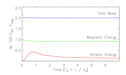
Figure 1: Evolution of total mass $M$ and kinetic and magnetic energies, $E_{kin}$ and $E_{mag}$ respectively. The kinetic energy $E_{kin}$ has been amplified by a factor of 100 to visualize its evolution more clearly. The resistivity in this model is $\eta=10^{-3}$ and the shear component of magnetic field $B_{z}=0.1$.

Figure 1 shows the evolution of total mass, kinetic and magnetic energies until the moment at which we start injecting the turbulence (i.e. $t=7$). All shown quantities, after some initial adaptation, reach steady, almost constant values. The near zero time derivatives of total mass, kinetic and magnetic energies guarantee the stationarity of the system. We remind the reader, that the system evolves in the presence of open boundary conditions, which could violate the conservation of mass and total energy. As we see, the conservation of these quantities is well satisfied during the Sweet-Parker stage in our models.

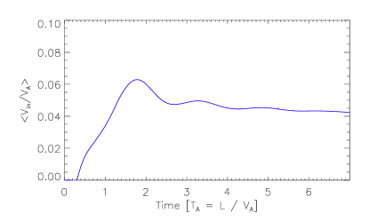
Figure 2: Evolution of the reconnection rate $\langle V_{in}/V_{A}\rangle$ for the same model as in Fig. 1. The reconnection rate grows initially until it reaches the stationary solution.

The reconnection rate, shown in Figure 2, also confirms that the evolution reaches a stationary state. Initially, the reconnection rate $\langle V_{in}/V_{A}\rangle$ grows until time $t\approx 1.8$, when it reaches the maximum value of $\approx 0.06$. Later on, it drops a bit approaching a value of $0.04$. During the last period of about 3 Alfvén time units, the change of the reconnection rate is very small. We assume that these conditions guarantee a nearly steady state evolution of the system, so at this point we are ready to introduce turbulence.

In Figure 3 we present the velocity and magnetic field configuration of the steady state. In the left panel of the figure we show the topology of velocity field as textures. The brightness of texture corresponds to the amplitude of velocity. The texture itself shows the direction of the field lines. The topology of the velocity field is mainly characterized by strong outflow regions along the mid-plane. The outflow is produced by the constant reconnection process at the diffusion region near the center and the ejection of the reconnected magnetic flux through the left and right boundaries. The system is in a steady state when the flux which reconnects is counterbalanced by the incoming fresh flux. The inflow is much slower then the outflow, but still its direction can be recognized from the texture shown in the left plot of Figure 3.

The topology of the magnetic field is presented in the middle panel of Figure 3. We recognize the anti-parallel configuration of the field lines with the uniform strength out of the mid-plane. Near the mid-plane, the horizontal magnetic lines are reconnected generating the Y-component, which is ejected by the strong outflow. In addition, we show the absolute value of current density in the right panel of Figure 3. We see very elongated diffusion region in the middle of the box, where reconnection takes place. The maximum value of $|\vec{j}|$ does not exceed a value of 25.

0.4.2 Effects of Turbulence

The essential part of our studies covers the effects of turbulence on reconnection. Our goal is to achieve a stationary state of Sweet-Parker reconnection, which is described in the previous subsection, and then introduce turbulence at a given injection scale $l_{inj}$, gradually increasing its strength to the desired amplitude corresponding to the turbulent power $P_{inj}$. We inject turbulence in the region surrounding the mid plane and extending to the distance of around one quarter of the size of the box. The transition period during which we increase the strength of turbulence, has length of one Alfvénic time and starts at $t=7$. It means that from $t=8$ we inject turbulence at maximum power $P_{inj}$.

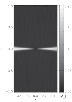
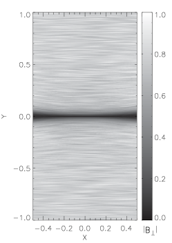
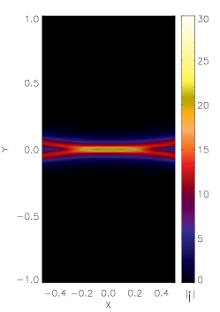
Figure 3: Topology and strength of velocity field (left panel) and magnetic field (middle panel) during the Sweet-Parker reconnection at $t=7$. In the right panel we show the absolute value of current density $\vec{j}$. The images show the XY-cut through the domain at $Z=0$.

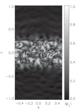
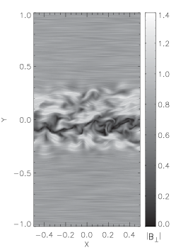
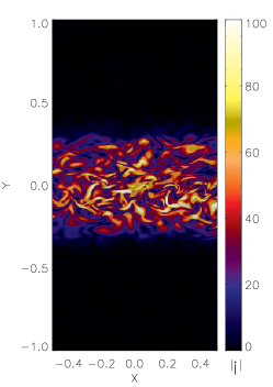
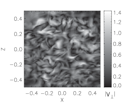
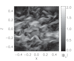
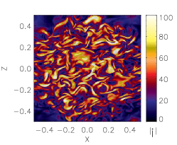
Figure 4: Topology and strength of velocity field (left panel) and magnetic field (middle panel) in the presence of fully developed turbulence at time $t=12$. In the right panel we show distribution of the absolute value of current density $|\vec{J}|$. The images show the XY-cut (upper row) and XZ-cut (lower row) of the domain at the midplane of the computational box. Turbulence is injected with the power $P_{inj}=1$ at scale $k_{inj}=8$.

In Figure 4 we show examples of XY-cuts (upper row) and XZ-cuts (lower row) through the box of the velocity (left panel) and magnetic field (middle panel) topologies with the intensities corresponding respectively to the amplitude of perpendicular components of velocity and magnetic field to the normal vector defining the plotted plane.

The first noticeable difference compared to the Sweet-Parker configuration is a significant change of the velocity and magnetic field topologies. Velocity has very complex and mixed structure near the mid plane, since we constantly inject turbulence in this region (see the left panel in Fig. 4). Although the structure is very complex here, most of the velocity fluctuations are pointed in the directions perpendicular to the mean magnetic field. This comes from the fact, that in the nearly incompressible regime of turbulence, most of the fluctuations propagate as Alfvén waves along the mean magnetic field. Slow and fast waves, whose strengths are significantly reduced, are allowed to propagate also in directions perpendicular to the mean field. As a result most of the turbulent kinetic energy leaves the box along the magnetic lines. The fluctuations, however, efficiently bend magnetic lines near the diffusion region. There, the strength of the magnetic field is reduced, since this is the place where magnetic lines change their directions (see the middle upper panel in Fig. 4). The interface between positively and negatively directed magnetic lines is much more complex then in the case of Sweet-Parker reconnection. This complexity favors creation of enhanced current density regions, where the local reconnection works faster since the current density reaches higher values (see the right panel of Fig. 4). Since we observe multiple reconnection events happening at the same time (compare the right panel of Fig. 4 to the Sweet-Parker case in Fig. 3), the total reconnection rate should be significantly enhanced.

Dependence on the Turbulent Power

We run several models with varying power of turbulence. All other parameters were kept the same. This allowed us to estimate the dependence of the reconnection rate on the power of injected turbulence.

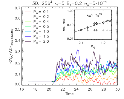
Figure 5: Time evolution of the reconnection speed $V_{rec}$ for models with different powers of turbulence $P_{inj}$ (see legend). In the subplot we show the dependence of $V_{rec}$ on $P_{inj}$.

Figure 5 shows the evolution of reconnection speed in models with the turbulent power $P_{inj}$ varying in the range of over one order of magnitude, from 0.1 to 2.0. The evolution of $V_{rec}$ reaches stationarity in a relatively short period of about one Alfvén time, estimated from the plot. In order to obtain the turbulent power dependence, we averaged $V_{rec}$ over a time interval starting from $t=21$ and ending at time $t=30$. In the subplot of Figure 5 we plot the dependence of the averaged reconnection speed on the strength of turbulence. Diamonds represent the averaged reconnection rate in the presence of turbulence. Pluses represent the reconnection rate during the Sweet-Parker process, i.e. without turbulence. The error bars correspond to the standard deviation of $V_{rec}$, which is a measure of time variation.

Fitting to the calculated points gives us a dependency of the reconnection speed $V_{rec}$ scaling with the power of turbulence as $\sim P_{inj}^{1/2}$. The power is proportional to $\sim V_{l}^{2}/t$ and $t\sim L/V_{l}\cdot V_{A}/V_{l}$, where $V_{l}$ is the amplitude of turbulence at the injection scale and $V_{A}$ is the Alfvén speed. This gives the relation $P_{inj}\sim V_{l}^{4}$, thus the dependency of the reconnection speed $V_{rec}$ on the amplitude of fluctuation at the injection scale $V_{l}$ is $V_{rec}\sim V_{l}^{2}$, which corresponds to the LV99 prediction.

Dependence on the Injection Scale

Similar studies have been done in order to derive the dependence of the reconnection speed $V_{rec}$ on the scale at which we inject turbulence, $l_{inj}$. Keeping the same power of turbulence for all models we inject turbulence at several scales, from $k_{f}=3$ to $k_{f}=12$. This limited range allows us to obtain desired dependence.

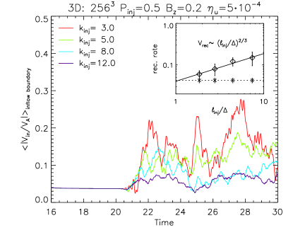
Figure 6: Time changes of the reconnection speed $V_{rec}$ for models with different injection scale $l_{inj}$. In the subplot we show the dependence of $V_{rec}$ on $l_{inj}$. $\Delta$ is the current sheet thickness, and it is assumed constant for all models.

In Figure 6 we present the results obtained in this series of models. From the plot we clearly see a strong dependence of the reconnection rate on the injection scale. The model with the injection at a smaller scale $k_{f}=12$ reaches smaller values of the reconnection rate. In the model with the injection at larger scale $k_{f}=3$, the reconnection is faster than the Sweet-Parker reconnection by a factor of almost 10 at some moments. After averaging the rates over time, we plot its dependence on the injection scale in the subplot of Figure 6.

The fitting to the relation of reconnection rate on the injection scale gives the dependency of $V_{rec}\sim l_{inj}^{2/3}$, which is stronger then predicted $\sim l_{inj}^{1/2}$ by LV99. In their paper, the authors considered Goldreich-Sridhar model of turbulence (Goldreich & Sridhar, 1995) starting at $l_{inj}$. The existence of the inverse cascade can modify the effective $l_{inj}$. In addition, reconnection can also modify the characteristics of turbulence. This aspect requires more study.

Dependence on Resistivity

In the global constraint of reconnection rate derived by LV99 there is no explicit dependency on the resistivity. In order to study this, we performed another set of models in which we changed the uniform resistivity $\eta$ only.

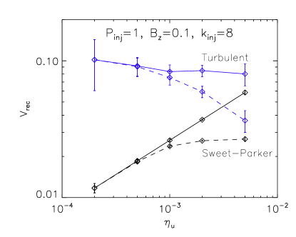
Figure 7: Dependence of the reconnection rate on the uniform resistivity. Black line shows Sweet-Parker reconnection rate, and blue line shows the reconnection rate in the presence of turbulence. Dashed lines show actual reconnection rates obtained from models. Solid lines show corrected speeds according to the procedure described in the text.

In Figure 7 we show reconnection rates obtained from this set of models. We plot $V_{rec}$ for five models with $\eta$ varying from $2\cdot 10^{-4}$ to $5\cdot 10^{-3}$. The dashed lines show relations obtained directly from simulations. Since our computational box does not change from model to model, the magnetic field has non-zero gradients at the boundaries for the higher values of resistivity. This affects the evolution by reducing the reconnection rate. We know from theory that the reconnection rate $V_{SP}$ during the Sweet-Parker stage scales as $\sim\eta^{1/2}$. Using this relation, we have calculated correction coefficients by taking the ratio of $\eta^{1/2}/V_{SP}$. Using these coefficients we correct values of reconnection rate obtained during the turbulent stage. The result is plotted with the solid blue line. The relation signifies virtually no dependence of the $V_{rec}$ on $\eta$. The correctness of this approach requires more study.

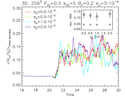
Figure 8: The evolution of the reconnection speed $V_{rec}$ for models with different anomalous resistivity $\eta_{a}$. In the subplot we show the dependence of $V_{rec}$ on $\eta_{a}$. Critical value of current density $j_{crit}$ is set to 25.0 in all models.

In addition to the uniform resistivity dependence, we have studied the dependence on the anomalous effects as well. The results of these studies are presented in Figure 8 and show four models with the same uniform resistivity $\eta_{u}=5\cdot 10^{-4}$ and the critical current density $j_{crit}=25.0$ but with the anomalous resistivity parameter $\eta_{a}$ varying between $0.0$ and $2\cdot 10^{-3}$. In the subplot of Figure 8 we plot the dependence of the reconnection rate on the anomalous resistivity parameter $\eta_{a}$. We see that the reconnection speed $V_{rec}$ is insensitive to the value of $\eta_{a}$ to within the variations of the reconnection rate in each model (see the error bars).

0.5 Discussion

In this paper we tested the model of reconnection proposed by LV99. Our results show the significant influence of the turbulence on the magnetic reconnection rate. The reconnection speed $V_{rec}$ (Eq. 1) shows dependence on the characteristics of the turbulence only, the rate of energy injection and the scale of injection. In particular, there is no explicit dependency on the resistivity.

Numerical testing of the reconnection model in LV99 is far from trivial. The model is intrinsically three dimensional. In order to develop a sufficient range of turbulent cascade before it reaches the scale of current sheet we have to use high resolution simulations. Higher resolution, in addition, minimizes the role of numerical diffusion. Another problem is the adaptation of proper boundary conditions. Our model requires open boundaries in order to allow the ejection of the reconnected flux. This type of boundary conditions should allow for free outflow of the matter and magnetic field. This property is crucial for the global reconnection constraint, since the reconnection stops when the outflow of reconnected flux is blocked.

Even though these numerical simulations allow us to study reconnection in the presence of turbulence for a limited range of magnetic Reynolds numbers (in this paper $R_{m}<10^{3}$), the results provide good testing of the relations derived by LV99. The strong dependence of $V_{rec}$ on the injection scale, when scaled to the real conditions of the interstellar medium, shows dramatic enhancement of the reconnection speed, which even in the presence of a magnetic field almost perfectly frozen in the medium, allows for fast reconnection with the characteristic time comparable to the Alfvén time. The LV99 model predicts this dependence to be as $V_{rec}\sim l_{inj}^{1/2}$. However, our numerical testings show a stronger dependence, $V_{rec}\sim l_{inj}^{2/3}$. This difference can be explained by the presence of the inverse cascade of turbulence in our numerical models.

The advantage of LV99 model is that it is robust and fast in any type of fluid, under the assumption that the fluid is turbulent. Consequences of this are dramatic. The reconnection process is not determined by Ohmic diffusion, but it is controlled by the characteristics of turbulence, like its strength and the energy injection scale. Turbulence efficiently removes the reconnected flux fulfilling the global constraint (Eq. 1). Our numerical results confirm the LV99 prediction of a strong dependence of the reconnection rate on the amplitude of turbulence, i.e. $V_{rec}\sim V_{l}^{2}$, but most importantly, they show that the reconnection in the presence of turbulence is not sensitive to the magnetic diffusivity of the medium.

0.6 Summary

In this article we investigated the influence of turbulence on the reconnection process using numerical experiments. This work is the first attempt to test numerically the model presented by Lazarian & Vishniac (1999). We analyzed the dependence of the reconnection process on the two main properties of turbulence, namely, its power and the injection scale. We also analyzed the role of Ohmic resistivity in the weakly turbulent reconnection. We found that:

• Numerical studies of stochastic reconnection are finally possible, even though reconnection in numerical simulations is always fast.

• Turbulence drastically changes the topology of magnetic field near the interface of oppositely directed magnetic field lines. These changes include the fragmentation of the current sheet which favors multiple simultaneous reconnection events.

• The reconnection rate is determined by the thickness of the outflow region. For large scale turbulence, the reconnection rate depends on the amplitude of fluctuations and injection scale as $V_{rec}\sim V_{l}^{2}$ and $V_{rec}\sim l_{inj}^{2/3}$, respectively.

• Reconnection in the presence of turbulence is not sensitive to Ohmic resistivity. The introduction of the anomalous resistivity does not change the rate of reconnection of weakly stochastic field either.