ABSOLUTE MAGNITUDE DISTRIBUTION AND LIGHT CURVES OF GAMMA-RAY BURST SUPERNOVAE

Abstract

Photometry data were collected from the literature and analyzed for supernovae that are thought to have a gamma–ray burst association. There are several gamma–ray bursts afterglow light curves that appear to have a supernova component. For these light curves, the supernova component was extracted and analyzed. A supernova light curve model was used to help determine the peak absolute magnitudes as well as estimates for the kinetic energy, ejected mass and nickel mass in the explosion. The peak absolute magnitudes are, on average, brighter than those of similar supernovae (stripped–envelope supernovae) that do not have a gamma–ray burst association, but this can easily be due to a selection effect. However, the kinetic energies and ejected masses were found to be considerably higher, on average, than those of similar supernovae without a gamma–ray burst association.

1 Introduction

A significant effort was made, over a number of years, to find the origin of gamma–ray bursts (GRBs). The discovery of optical afterglows in long–duration GRBs allowed for the determination of the GRB’s redshift (for a review, see van Paradijs, et al., 2000, and references therein). This led to the realization that long–duration GRBs are at cosmological distances (e.g., van Paradijs, et al., 1997; Metzger et al., 1997). In this paper, long–duration, cosmological GRBs will be referred to simply as GRBs.

The light curve of the optical afterglow of GRB 980326 showed a rebrightening at around two weeks after the burst (Bloom et al., 1999). This rebrightening, or bump, in the light curve was attributed to an underlying supernova (SN). This was the first observational indication of an association between GRBs and SNe.

During April of 1998, an unusual gamma–ray burst, GRB 980425, was discovered with its gamma–ray energy several orders of magnitude lower than typical GRBs (Soffitta et al., 1998; Woosley et al., 1999). Optical observations of the region led to the discovery of an unusual supernova, SN 1998bw, within the error radius of the GRB (Galama et al., 1998). Spectra of SN 1998bw showed it to be a Type Ic SN with exceptionally broad lines (Ic–BL). This SN was also unusually bright for a Type Ic SN (Richardson et al., 2006). It was thought that GRB 980425 might simply be a normal GRB, but one where the jet was viewed off axis (e.g. Nakamura, 1999; Ioka & Nakamura, 2001; Yamazaki et al., 2003). However, according to late–time radio observations (Soderberg et al., 2004), even if it was viewed off–axis it would still be an unusual GRB. There may be more dim, peculiar GRBs, like GRB 980425, than observations would indicate; due to the fact that those at large redshifts are difficult to detect.

The afterglow spectra of GRB 030329 were remarkably similar to that of SN 1998bw (Stanek et al., 2003). The SN associated with this GRB was then named SN 2003dh. From this, it was clear that at least some long–duration gamma–ray bursts are connected to supernovae. Since then, two other SNe Ic–BL have been spectroscopically confirmed to have a GRB connection: SN 2003lw/GRB 031203 (Malesani et al., 2004) and SN 2006aj/GRB 060218 (Sollerman et al., 2006; Mazzali et al., 2006b; Modjaz et al., 2006; Mirabal et al., 2006). Not all SNe Ic–BL have a convincing GRB connection; as is the case for SN 1997ef (Iwamoto et al., 2000) and SN 2002ap (Mazzali et al., 2002). However, this does not rule out the possibility of an association with a weak (possibly off–axis) GRB. It also seems that there are some long–duration gamma–ray bursts with no apparent associated supernova; such as GRBs 060505 and 060614 (Fynbo et al., 2006).

Similar to the bump found in the optical afterglow light curve of GRB 980326 (mentioned above), there have been several other GRB afterglow light curves with just such a bump (e.g., Reichart, 1999; Galama et al., 2000; Sahu et al., 2000; Castro-Tirado et al., 2001). This provides us with a number of possible GRB/SNe to consider, even without spectroscopic confirmation. These light curves are typically analyzed using a composite model (e.g. Zeh et al., 2004; Bloom, 2004; Stanek et al., 2005), discussed below in Section 5. Most of the light curves considered here are of this type. For alternative explanations for this rebrightening see Fynbo et al. (2004) and references therein. For a discussion on the possible progenitors of long–duration GRBs, see Fryer et al. (2007). The observed data are discussed in Section 2. Section 3 covers the analysis of the light curves while the results are presented in Section 4. The conclusions are discussed in Section 5.

2 Data

The photometry data were collected from the literature. R–band data were used for most of the GRBs due to their relatively high redshifts. V–band data were used for GRB 980425 ($z=0.00841$) and GRB 060218 ($z=0.0331$). The photometry references are given in Table 1.

Distances and extinctions were taken into account in order to convert the apparent magnitudes to absolute magnitudes. Luminosity distances were calculated from the redshifts using the following cosmology: H${}_{0}=60$ $km\ s^{-1}Mpc^{-1}$, $\Omega_{M}=0.3$ and $\Omega_{\Lambda}=0.7$. The distance modulus, $\mu$, for each GRB was calculated and is given in Table 1 along with the references.

Foreground Galactic extinction was taken into account according to Schlegel et al. (1998). These values were taken from NED and converted from A_B to A_V. For host galaxy extinction, the best estimates from the literature were used. In the case where the host galaxy extinction was estimated to be small or negligible (yet still unknown), a value of 0.05 mag was assigned. The extinctions are listed in Table 1, along with their references.

Spectra of SN 1998bw were used to calculate K–corrections. The spectra used were from Patat et al. (2001) and obtained from the SUSPECT database.

3 Analysis

Three of the light curves used in this study had no significant GRB afterglow component at the time of the SN: GRB 980425/SN 1998bw, GRB 031203/SN 2003lw and GRB 060218/SN 2006aj. One of the light curves (GRB 030329/SN 2003dh) had no noticeable SN bump; that is to say that the SN component was masked by a slowly declining afterglow. However, spectroscopy revealed a significant SN contribution (Stanek et al., 2003). Most of the light curves had both a SN bump and a significant GRB afterglow component at the time of the SN. In order to analyze the SN by itself, the GRB afterglow component (and sometimes the host galaxy contribution) needed to be removed. If the light curve still included light from the host galaxy, and yet there was not sufficient late–time data to determine the host galaxy contribution, then that GRB was not included in the study. This was the case for GRB 991208.

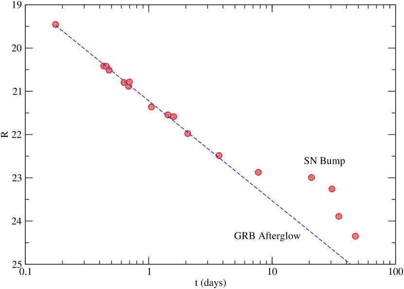
Figure 1: The observed R–band light curve of GRB 990712 after the host galaxy light had been subtracted. The diagonal dashed line represents the contribution due to the GRB afterglow. In this particular case, the afterglow light can be described by the equation: $R_{AG}=2.31log(t)+21.22$.

Once the host galaxy light had been accounted for, there were still two components. The GRB and the SN were treated independent of each other. While there is certainly some interaction between the GRB and the SN, treating them as independent is a reasonable first order approximation. The early–time data, in the resulting light curve, were used to determine the contribution of the GRB afterglow. After day one, or day two, this was usually an unbroken power law. It appears as a straight line on a graph of R vs. log(t), as shown in Figure 1. The only exception is GRB 030329, where the GRB afterglow contribution was determined solely from the spectra. For all other GRBs, there needed to be sufficient early–time data to determine the GRB afterglow contribution. If this contribution could not sufficiently be determined from the data, then that GRB was not used in this study. This was the case for GRB 010921 and GRB 000911.

There were, however, a few exceptions (GRBs 020305, 020410 and 020903). The two dimmest SNe in the study are from the light curves of GRB 020305 and GRB 020410. If the actual GRB contribution was larger than estimated for these SNe (shallower slope), then the SN contribution would be smaller making these SNe even dimmer than reported here. Even if the GRB contribution was negligible (steeper slope, including a downward break), then these two SNe would be brighter than reported here, but would still be the two dimmest SNe in the study. The light curve of GRB 020903 was not sufficient to get a good estimate of the GRB contribution. However, it was sufficient to reasonably determine that the GRB afterglow had a negligible contribution at the time of the SN’s peak brightness. These three SNe are included because their peak absolute magnitudes are still relevant, even if the other information obtained from the light curve fitting remains highly uncertain (see Table 2). In general, the uncertainty in determining the GRB afterglow contribution is difficult to quantify and has not been included in the peak absolute–magnitude uncertainties given in Table 2.

3.1 Model

A SN light–curve model was used to help obtain accurate peak absolute magnitudes from the resulting light curves. It was also used in determining estimates of the kinetic energy, ejected mass and nickel mass for each SN. The model used here is a semi–analytical model derived from two already existing models; Arnett (1982) and Jeffery (1999). At early times, the Arnett model is used; where the diffusion approximation is valid. At late times, the deposition of gamma–rays dominates the light curve, and the Jeffery model accounts for this. The basic assumptions are spherical symmetry; homologous expansion; radiation pressure dominance at early times; that ⁵⁶Ni exists and has a distribution that is somewhat peaked toward the center of the ejected matter. Also, optical opacity is assumed to be constant at early times and gamma-ray opacity is assumed to be constant at late times. The combined model is described in detail by Richardson et al. (2006).

The model uses the SN’s kinetic energy, ejected mass and nickel mass as parameters. After searching a grid of parameter values, a least–squares best fit was used to determine the most likely parameter values for each light curve. In order to improve the results, the ratio of kinetic energy to ejected mass was constrained. SN spectra were used to determine this ratio; however, spectra exist for only four of the GRB/SNe in the study. These ratios are given in foe M${}_{\odot}^{-1}$, where 1 foe $=10^{51}$ erg. The values are 5.0 for SN 1998bw (Nakamura et al., 2001), 4.8 for SN 2003dh (Mazzali et al., 2003), 4.6 for SN 2003lw (Mazzali et al., 2006a) and 1.0 for SN 2006aj (Mazzali et al., 2006b). The average of these four values, 3.8, was used for the other GRB/SNe for which spectra were not available. Possible consequences of this approximation are discussed below (Section 4.2).

4 Results

4.1 Absolute–Magnitude Distribution

The peak absolute magnitudes are listed in Table 2. The uncertainties shown were obtained by taking into account the uncertainties for each of the values in Table 1, as well as the observational uncertainties in the apparent magnitudes. Figure 2 shows a histogram of the absolute–magnitude distribution. This distribution has an average of M${}_{V,peak}=-19.2\pm 0.2$ and a standard deviation of $\sigma=0.7$. Also shown in this figure is the distribution of stripped–envelope SNe, (Richardson et al., 2006, Fig. 2). Stripped–envelope SNe (SE SNe) are a combination of SNe Ib, Ic and IIb; and those shown here, do not have a GRB association. The main difference between these two distributions is that the GRB/SNe are, on average, brighter by 0.8 magnitudes. This is likely due to a selection effect. In order for most of the GRB/SNe to be detected, they have to be relatively bright compared to their GRB afterglow. Otherwise, it must be close enough to obtain a spectrum; as was the case with GRB 030329. Therefore, any relatively distant SN connected with a GRB that has a bright, or slowly declining, afterglow will not be detected; especially if the SN is relatively dim. This is why the dim GRB/SNe are likely to be undercounted. Notice that the two dim GRB/SNe fit well within the SE SN distribution.

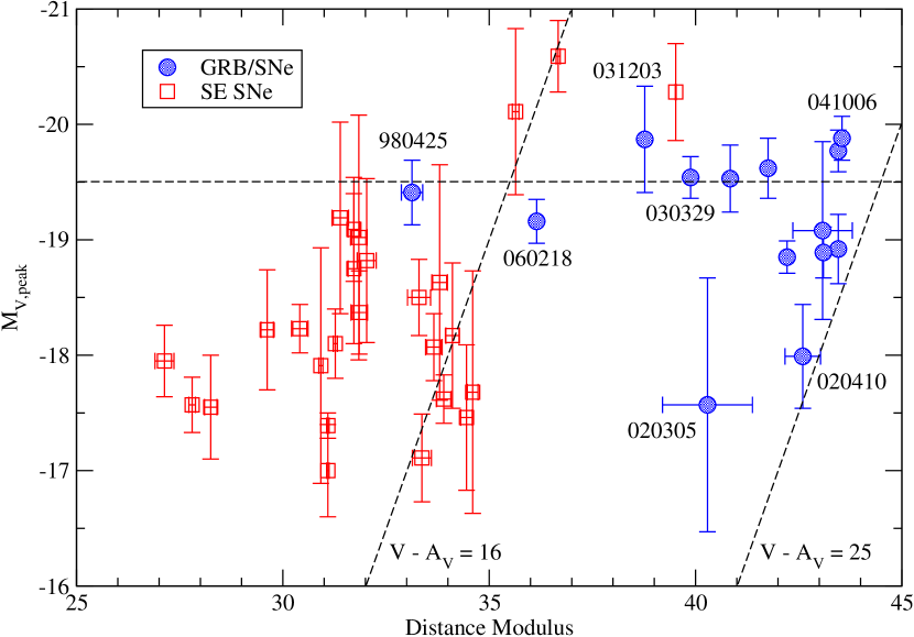
Figure 3: Peak absolute–magnitude is plotted here versus distance modulus. The diagonal dashed lines are lines of constant apparent magnitude (16 and 25 mag.). The dashed horizontal line at $M_{V}=-19.5$, representing the SN Ia ridge line, is shown for comparison. The filled circles are GRB/SNe and the open squares are SE SNe. The associated GRB names are used to label a few key GRB/SNe.

A graph of peak absolute magnitude versus distance modulus is shown in Figure 3. The two diagonal dashed lines represent the apparent magnitudes of 16 and 25. The horizontal dashed line represents the Type Ia ridge line, and is shown for comparison. The GRB/SNe can be compared to SE SNe (Richardson et al., 2006), included in this graph. Nearly all of the GRB/SNe were found to have an apparent magnitude dimmer than 16, but with a limiting magnitude of 25. This is in contrast to the SE SNe which were nearly all found to have an apparent magnitude brighter than 16. Since this is related to distance, we see that it is rare to find any nearby GRB/SNe. Distant GRB/SNe are discovered because their associated GRBs are extremely bright.

About half of the GRB/SNe in Figure 3 are near the Type Ia ridge line. The dimmest SN in the study, from GRB 020305, has a very large uncertainty. It is still worth including, however, due to the fact that it is firmly at the low end of the distribution even with the large uncertainty.

When compared to other studies, the absolute magnitudes given here are, on average, somewhat brighter (after accounting for different cosmologies). For example, see Table 5 from Soderberg et al. (2006) and Figure 6 (which is similar to Figure 3 of this paper) from Ferrero et al. (2006). This difference could possibly be due to the different methods for extracting the peak absolute magnitudes.

4.2 Light Curves

The light curves are presented in Figure 4. Most of these light curves have a good range over time, considering the difficulty in separating the SN contribution from that of the GRB afterglow (early times) and host galaxy (late times).

The best estimates for kinetic energy, ejected mass and nickel mass are given in Table 2, along with rise times. Because spectra exists for only four of these GRB/SNe, E${}_{k}/$M_ej values are only known for these four. The average value is used for the others. This is a reasonable first order estimate; however, a change in this value affects the individual E_k and M_ej values determined by the model. The trend is that increasing the E${}_{k}/$M_ej ratio leads to an increase in both the E_k and M_ej values obtained in the best model fits. This does not significantly affect the M_Ni values and therefore does not affect M_V,peak. Also notice, from Table 2, that M_V,peak and E_k are not correlated. This was the case for SE SNe as well (Richardson et al., 2006). Note that in the light–curve model, it is assumed that a substantial amount of ⁵⁶Ni is synthesized in the explosion. The decay of this isotope powers the peak of the light curve. Then, ⁵⁶Co (which is a product of the ⁵⁶Ni decay) itself decays and powers the tail of the light curve.

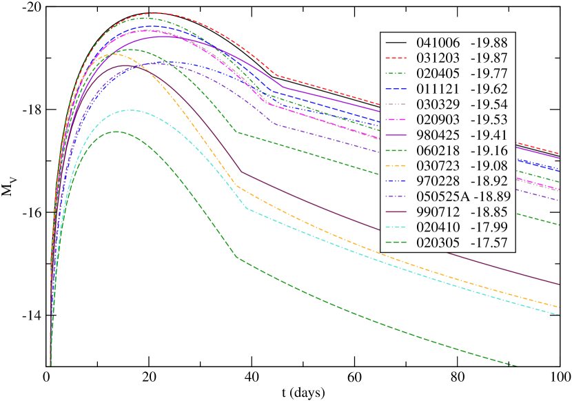
Figure 5: All of the GRB/SN model light curves in the study are plotted here. The peak absolute magnitudes are given for each.

The best fit model light curves are all shown on the same graph in Figure 5, with a common time of explosion. This shows, as expected, a general trend that the brighter SNe have broader light curves. This, however, is not always the case. GRB 030723 is very narrow compared to GRB 970228, yet they have similar peak magnitudes.

5 Conclusions

The average peak absolute magnitude was found to be higher for the GRB/SNe than for the SE SNe. However, in view of possible selection effects, the difference may not be significant. There were two GRB/SNe at the dim end of the distribution, but well within the distribution of SE SNe.

Most of the SN data analyzed here were taken from GRB afterglow light curves. The GRB light was treated as being independent of the SN light and was removed so that the resulting light curve could be analyzed as a SN light curve. These resulting light curves fit quite well with a SN light curve model (Figure 4).

GRB afterglow light curves that are suspected of having a SN component are usually analyzed by a different method. Usually the observed data are fit to a composite model, where all of the components are represented; GRB, SN and host galaxy (Zeh et al., 2004, for example). The assumptions made are similar to those made with the separation method of this paper. The main difference between the two methods is in the way the SN is treated. The composite method starts with a light curve of SN 1998bw (adjusted for the GRBs redshift). Two of the five free parameters in the composite model are then used in the overall fit to describe the SN; one for the brightness and one for the width of the SN contribution. While the separation method uses SN 1998bw for K–corrections, a general SE SN model is then fit to the resulting light curve. The two methods are similar; however, the separation method used here allows for closer analysis of the the SN. Reasonable estimates of the kinetic energy, ejected mass, nickel mass and rise times are found. However, the values of kinetic energy and ejected mass from other studies (Nomoto, 2006) tend to be larger by a factor of approximately two.

The coincidence of the GRB date and the derived date of the SN explosion is another point of interest. In all but two cases the difference between the two dates was less than a week. For GRB 050525A, the SN explosion date is estimated to have occurred about 10 days before the GRB date, but by looking at the model fit and the observed data in Figure 4, we see that the model was not able to simultaneously reproduce the narrow peak and the bright, late–time data point. It appears that a more accurate explosion date for the SN would bring it closer to the GRB date. For GRB 011121, the SN explosion date is estimated to have occurred about 9 days before the GRB date. Other studies have given similar results (Bloom et al., 2002), but the lack of pre–peak data for this SN makes the SN explosion date difficult to accurately pin down. Thus there is no clear evidence for real differences between the times of the GRBs and the SNe.

The nickel masses determined here range from 0.05 to 0.99 M_⊙. These are similar to the values found for SE SNe with no GRB association (Richardson et al., 2006). However, the kinetic energy values determined here range from about one to 31 foe and the ejected mass values range from about one to six M_⊙. These values are, on average, considerably higher than those found for SE SNe with no GRB association.

Table 1: Data Used In Determining Absolute Magnitudes

GRB/	Photometry	$\mu^{a}$	Ref.	A${}_{R}(Galactic)^{b}$	A${}_{V}(host)$	Ref.
XRF	Ref.	(mag)		(mag)	(mag)
970228	1	43.463 $\pm$ 0.003	2	0.543 $\pm$ 0.087	0.15 $\pm$ 0.15	3
980425	4,5,6	33.13 $\pm$ 0.26	7	0.194 $\pm$ 0.031c	0.05 $\pm$ 0.05	8
990712	9,10	42.224 $\pm$ 0.005	11	0.090 $\pm$ 0.014	0.15 $\pm$ 0.1	12
011121	13,14	41.764 $\pm$ 0.006	14	1.325 $\pm$ 0.212	0.05 $\pm$ 0.05	14
020305	15	40.29 $\pm$ 1.09	15	0.142 $\pm$ 0.023	0.05 $\pm$ 0.05	15
020405	16	43.463 $\pm$ 0.016	16	0.146 $\pm$ 0.023	0.15 $\pm$ 0.15	17
020410	18	42.60 $\pm$ 0.43	18	0.398 $\pm$ 0.064	0.05 $\pm$ 0.05	18
020903	19	40.844 $\pm$ 0.003	19	0.0935 $\pm$ 0.0150	0.26 $\pm$ 0.26	19
030329	20	39.88 $\pm$ 0.01	21	0.0675 $\pm$ 0.0108	0.39 $\pm$ 0.15	17
030723	22	43.08 $\pm$ 0.72	23	0.0886 $\pm$ 0.0142	0.23 $\pm$ 0.23	22
031203	24	38.775 $\pm$ 0.003	25	2.772 $\pm$ 0.444	0.05 $\pm$ 0.05	26
041006	27	43.55 $\pm$ 0.03	27	0.0607 $\pm$ 0.0097	0.11 $\pm$ 0.11	17
050525A	28	43.10 $\pm$ 0.07	29	0.2546 $\pm$ 0.0407	0.12 $\pm$ 0.06	30
060218	31	36.15 $\pm$ 0.05	31	0.471 $\pm$ 0.075c	0.13 $\pm$ 0.13	31

References. — (1) Galama et al. (2000), (2) Bloom et al. (2001), (3) Castander and Lamb (1999), (4) Galama et al. (1998), (5) McKenzie & Schaefer (1999), (6) Sollerman et al. (2000), (7) Kay et al. (1998), (8) Nakamura et al. (2001), (9) Sahu et al. (2000), (10) Fruchter et al. (2000), (11) NED, (12) Christensen et al. (2004), (13) Bloom et al. (2002), (14) Garnavich et al. (2003), (15) Gorosabel et al. (2005), (16) Masetti et al. (2003), (17) Kann et al. (2006), (18) Levan et al. (2005), (19) Bersier et al. (2006), (20) Matheson et al. (2003), (21) Greiner et al. (2003), (22) Fynbo et al. (2004), (23) Tominaga et al. (2004), (24) Malesani et al. (2004), (25) Prochaska et al. (2004), (26) Mazzali et al. (2006a), (27) Stanek et al. (2005), (28) Della Valle et al. (2006), (29) Foley et al. (2005), (30) Blustin et al. (2006), (31) Sollerman et al. (2006)

Table 2: Results

GRB/	MV,peak	Ek	Mej	MNi	trise	N
XRF	(mag)	(foe)	(M⊙)	(M⊙)	(days)
970228	$-18.9\pm 0.3$	23.2	6.11	0.54	24	4
980425	$-19.4\pm 0.3$	31.0	6.22	0.78	23	104
990712	$-18.9\pm 0.1$	5.32	1.40	0.20	15	5
011121	$-19.6\pm 0.3$	14.2	3.73	0.73	21	9
020305	$-17.6\pm 1.1$	3.61a	0.95a	0.05	14a	7
020405	$-19.8\pm 0.2$	11.1	2.92	0.72	19	5
020410	$-18.0\pm 0.4$	6.42a	1.69a	0.10	16a	3
020903	$-19.5\pm 0.3$	11.9a	3.13a	0.60	20a	11
030329	$-19.5\pm 0.2$	17.4	3.63	0.62	20	17
030723	$-19.1\pm 0.8$	3.23	0.85	0.19	13	9
031203	$-19.9\pm 0.5$	21.0	4.56	0.99	21	10
041006	$-19.9\pm 0.2$	14.5	3.81	0.94	21	5
050525A	$-18.9\pm 0.2$	15.7	4.14	0.40	21	7
060218	$-19.2\pm 0.2$	0.89	0.89	0.30	16	42

Figure 2: The peak absolute–magnitude distribution for GRB/SNe (solid bars) is shown with an average value of $M_{V,peak}=-19.2\pm 0.2$ and a standard deviation of $\sigma=0.7$. SE SNe are shown for comparison (striped bars).

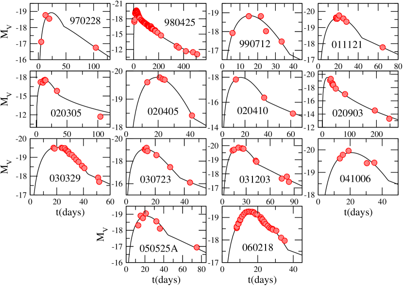
Figure 4: All of the GRB/SN light curves in the study are plotted here with the best model fits.

References

- Arnett (1982) Arnett, D. 1982, ApJ, 253, 785
- Bersier et al. (2006) Bersier, D., et al. 2006, ApJ, 643, 284
- Bloom et al. (1999) Bloom, J. S., et al. 1999, Nature, 401, 453
- Bloom et al. (2001) Bloom, J. S., Djorgovski, S. G., & Kulkarni, S. R. 2001, ApJ, 554, 678
- Bloom et al. (2002) Bloom, J. S., et al. 2002, ApJ, 572, L45
- Bloom (2004) Bloom, J. S. 2004, in ASP Conf. Ser. 312, Gamma Ray Bursts in the Afterglow Era, ed. M. Feroci et al. (San Francisco: ASP), 257
- Blustin et al. (2006) Blustin, A., et al. 2006, ApJ, 637, 901
- Castander and Lamb (1999) Castander, F., & Lamb, D. 1999, ApJ, 523, 593
- Castro-Tirado et al. (2001) Castro-Tirado, A., et al. 2001, A&A, 370, 398
- Christensen et al. (2004) Christensen, L., Hjorth, J., Gorosabel, J., Vreeswijk, P., Fruchter, A., Sahu, K., & Petro, L. 2004, A&A, 413, 121
- Della Valle et al. (2006) Della Valle, M., et al. 2006, ApJ, 642, L103
- Ferrero et al. (2006) Ferrero, P., et al. 2006, A&A, 457, 857
- Foley et al. (2005) Foley, R., Chen, H., Bloom, J., & Prochaska, J. 2005, GCN, 3483
- Fruchter et al. (2000) Fruchter, A., Vreeswijk, P., Hook, R., & Pian, E. 2000, GCN, 752
- Fryer et al. (2007) Fryer, C., et al. 2007, PASP, 119, 1211
- Fynbo et al. (2004) Fynbo, J. P. U., et al. 2004, ApJ, 609, 962
- Fynbo et al. (2006) Fynbo J. P., et al. 2006, Nature, 444, 21
- Galama et al. (1998) Galama, T., et al. 1998, Nature, 395, 670
- Galama et al. (2000) Galama, T., et al. 2000, ApJ, 536, 185
- Garnavich et al. (2003) Garnavich, P., et al. 2003, ApJ, 582, 924
- Gorosabel et al. (2005) Gorosabel, J., et al. 2005, A&A, 437, 411
- Greiner et al. (2003) Greiner, J., et al. 2003, GCN, 2020
- Ioka & Nakamura (2001) Ioka, K., & Nakamura, T. 2001, ApJ, 554, L163
- Iwamoto et al. (2000) Iwamoto, K., et al. 2000, ApJ, 534, 660
- Jeffery (1999) Jeffery, D. 1999, preprint (astro-ph/9907015)
- Kann et al. (2006) Kann, D., Klose, S., & Zeh, A. 2006, ApJ, 641, 993
- Kay et al. (1998) Kay, L., Halpern, J., & Leighly, K. 1998 IAU Circ. 6969
- Levan et al. (2005) Levan, A., et al. 2005, ApJ, 624, 880
- Malesani et al. (2004) Malesani, D., et al. 2004, ApJ, 609, L5
- Masetti et al. (2003) Masetti, N., et al. 2003, A&A, 404, 465
- Matheson et al. (2003) Matheson, T., et al. 2003, ApJ, 599, 394
- Mazzali et al. (2002) Mazzali, P., et al. 2002, ApJ, 572, L61
- Mazzali et al. (2003) Mazzali, P., et al. 2003, ApJ, 599, L95
- Mazzali et al. (2006a) Mazzali, P., et al. 2006a, ApJ, 645, 1323
- Mazzali et al. (2006b) Mazzali, P., et al. 2006b, Nature, 442, 1018
- McKenzie & Schaefer (1999) McKenzie, E., & Schaefer, B. 1999, PASP, 111, 964
- Metzger et al. (1997) Metzger, M., Djorgovski, S., Kulkarni, S., Steidel, C., Adelberger, K., Frail, D., Costa, E., & Frontera, F. 1997, Nature, 387, 878
- Mirabal et al. (2006) Mirabal, N., Halpern, J., An, D., Thornstensen, J., & Terndrup, D. 2006, ApJ, 643, L99
- Modjaz et al. (2006) Modjaz, M., et al. 2006, ApJ, 645, L21
- Nakamura (1999) Nakamura, T. 1999, ApJ, 522, L101 ,
- Nakamura et al. (2001) Nakamura, T., Mazzali, P., Nomoto, K., & Iwamoto, K. 2001, ApJ, 550, 991
- Nomoto (2006) Nomoto, K., Tominaga, N., Tanaka, M., Maeda, K., Suzuki, T., Deng, J. S., & Mazzali, P. A. 2006, Il Nuovo Cimento B, 121, 1207
- Patat et al. (2001) Patat, F., et al. 2001, ApJ, 555, 900
- Prochaska et al. (2004) Prochaska, J. et al. 2004, ApJ, 611, 200
- Reichart (1999) Reichart, D. 1999, ApJ, 521, L111
- Richardson et al. (2006) Richardson, D., Branch, D., & Baron, E. 2006, AJ, 131, 2233
- Sahu et al. (2000) Sahu, K. et al. 2000, ApJ, 540, 74
- Schlegel et al. (1998) Schlegel, D., Finkbeiner, D., & Davis, M. 1998, ApJ, 500, 525
- Soderberg et al. (2004) Soderberg, A., Frail, D., & Wieringa, M. 2004, ApJ, 607, L13
- Soderberg et al. (2006) Soderberg, A., et al. 2006, ApJ, 636, 391
- Soffitta et al. (1998) Soffitta, P., et al. 1998, IAU Circ., 6884
- Sollerman et al. (2000) Sollerman, J., Kozma, C., Fransson, C., Leibundgut, B., Lundqvist, P., Ryde, F., & Woudt, P. 2000, ApJ, 537, L127
- Sollerman et al. (2006) Sollerman, J., et al. 2006, A&A, 454, 503
- Stanek et al. (2003) Stanek, K. Z., et al. 2003, ApJ, 591, L17
- Stanek et al. (2005) Stanek, K. Z., et al. 2005, ApJ, 626, L5
- Tominaga et al. (2004) Tominaga, N., Deng, J., Mazzali, P. A., Maeda, K., Nomoto, K., Pian, E., Hjorth, J., & Fynbo, J. P. U. 2004, ApJ, 612, L105
- van Paradijs, et al. (1997) van Parakijs, J., et al. 1997, Nature, 386, 686
- van Paradijs, et al. (2000) van Parakijs, J., Kouveliotou, C., & Wijers, R. 2000, ARA&A, 38, 379
- Woosley et al. (1999) Woosley, S., Eastman, R., & Schmidt, B. 1999, ApJ, 516, 788
- Yamazaki et al. (2003) Yamazaki, R., Yonetoku, D., & Nakamura, T. 2003, ApJ, 594, L79
- Zeh et al. (2004) Zeh, A., Klose, S., & Hartmann, D. 2004, ApJ, 609, 952