Measurement of the Slope Parameter $\alpha$ for the $\eta\to 3\pi^{0}$ decay with the Crystal Ball detector at the Mainz Microtron (MAMI-C)

Abstract

The dynamics of the $\eta\to 3\pi^{0}$ decay have been studied with the Crystal Ball multiphoton spectrometer and the TAPS calorimeter. Bremsstrahlung photons produced by the 1.5-GeV electron beam of the Mainz microtron MAMI-C and tagged by the Glasgow photon spectrometer were used for $\eta$-meson production. The analysis of $3\times 10^{6}$ $\gamma p\to\eta p\to 3\pi^{0}p\to 6\gamma p$ events yields the value $\alpha=-0.032\pm 0.003$ for the $\eta\to 3\pi^{0}$ slope parameter, which agrees with the majority of recent experimental results and has the smallest uncertainty. The $\pi^{0}\pi^{0}$ invariant-mass spectrum was investigated for the occurrence of a cusplike structure in the vicinity of the $\pi^{+}\pi^{-}$ threshold. The observed effect is small and does not affect our measured value for the slope parameter.

I Introduction

The experimental study of the simple and pure strong-interaction reaction

$$\pi^{0}\pi^{0}\to\pi^{0}\pi^{0}$$ (1)

is a real challenge as neither a $\pi^{0}$ target nor a $\pi^{0}$ beam is available. The properties of reaction (1) can be extracted indirectly from complicated processes, for example, from $K^{+}\to\pi^{0}\pi^{0}e^{+}\nu_{e}$ ($K^{+}_{e4}$), which is the weak decay of the $K^{+}$ followed by strong final-state interactions between the two $\pi^{0}$s. Major disadvantages of studying reaction (1) in $K^{+}_{e4}$ are the small branching ratio ($2.2\times 10^{-5}$) and the complications from the four complex form factors for the $K^{+}_{e4}$ decay amplitude needed to describe the four-particle final state.

Figure 1: Distributions for the phase-space decay of $\eta\to 3\pi^{0}$ (i.e., when $\alpha=0$) obtained from a Monte Carlo simulation: (a) Dalitz plot, where variable $T_{i}^{\pi}$ is the kinetic energy of each of the three pions and $\langle T^{\pi}\rangle$ is the mean kinetic energy of the three pions (with all energies being calculated in the $\eta$ rest frame); (b) variable $z=\rho^{2}/\rho^{2}_{\mathrm{max}}$, reflecting the density of the Dalitz plot.

Another process that can be used for the indirect study of reaction (1) is the decay

$$\eta\to 3\pi^{0}~{},$$ (2)

where the $\pi^{0}\pi^{0}$ final-state interaction can be seen in a difference of the $\eta\to 3\pi^{0}$ decay amplitude from phase space. The experimental study of this decay has several major advantages: the relatively large branching ratio for $\eta\to 3\pi^{0}$ (32.5%), a high yield of $\eta$ mesons in many production reactions, and very small background from other $3\pi^{0}$ contributions, especially in $\eta$ production close to the threshold.

Due to the low energies of the decay $\pi^{0}$s, $\pi^{0}\pi^{0}$ rescattering in $\eta\to 3\pi^{0}$ is expected to be dominated by S and P waves. This leads to the parametrization of the $\eta\to 3\pi^{0}$ decay amplitude as $A(\eta\to 3\pi^{0})\sim 1+\alpha z$ PDG , where $\alpha$ is the quadratic slope parameter that describes the difference from phase space. A convenient definition of the kinematic variable $z$ is

$$z=6\sum_{i=1}^{3}(E_{i}-m_{\eta}/3)^{2}/(m_{\eta}-3m_{\pi^{0}})^{2}=\rho^{2}/\rho^{2}_{\mathrm{max}}~{},$$ (3)

where $E_{i}$ is the energy of the $i$th pion in the $\eta$ rest frame, and $\rho$ is the distance from the center of the $\eta\to 3\pi^{0}$ Dalitz plot. The variable $z$ varies from 0, when all three $\pi^{0}$s have the same energy of $m_{\eta}/3$, to 1, when one $\pi^{0}$ is at rest. A geometrical interpretation of Eq. (3) gives $z=0$ when $\rho=0$ and $z=1$ when $\rho=\rho_{\mathrm{max}}$. The density of the $\eta\to 3\pi^{0}$ Dalitz plot is described by $|A(\eta\to 3\pi^{0})|^{2}\sim 1+2\alpha z$. The phase-space decay of $\eta\to 3\pi^{0}$ (i.e., when $\alpha=0$) gives a uniform density of the Dalitz plot, as shown in Fig. 1(a). The corresponding distribution of the variable $z$ is shown in Fig. 1(b); it is uniform for $z$ from 0 to $\approx$0.75 . Experimentally, the slope parameter $\alpha$ is usually determined from the deviation of the measured $z$ distribution from the corresponding distribution obtained by a Monte Carlo simulation in which the $\eta\to 3\pi^{0}$ decay amplitude is independent of $z$.

The $\eta\to 3\pi^{0}$ decay, which violates G parity, occurs mostly because of the $u$-$d$ quark mass difference. The precision measurement of the $\eta\to 3\pi^{0}$ decay width, $\Gamma(\eta\to 3\pi^{0})\sim(m_{d}-m_{u})^{2}(1+2\alpha z)$, and the parameter $\alpha$ are important tests of Chiral Perturbation Theory ($\chi$PTh) gasser ; kambor . In the $\chi$PTh momentum expansion in orders of the $\chi$PTh parameter $\sf p$, the leading ${\cal O}({\sf p}^{2})$ term of the decay amplitude explicitly depends on $m_{d}-m_{u}$. However, including this term and the second-order counter terms, ${\cal O}({\sf p}^{4})$, is not sufficient gasser to yield a decay width that is close to the measured value of 423 eV PDG . The use of dispersion relations kambor ; anisovich , which include pion rescattering to all orders, partially improves the agreement with the experimental value. For the parameter $\alpha$, the dispersion-relation calculations of Ref. kambor give a negative value in the range $-0.007$ to $-0.0014$, depending on the assumptions made. The results of these calculations are outside the value of $\alpha=-0.031\pm 0.004$ adopted by the Particle Data Group (PDG) PDG . This value for $\alpha$ is based on the analysis of $0.9\times 10^{6}$ $\eta\to 3\pi^{0}$ decays measured by the Crystal Ball at the AGS eta_slope_bnl . A complete two-loop calculation in standard $\chi$PTh Bijnens results in $\alpha=0.013\pm 0.032$, the sign of which is even opposite to the experimental values. The evaluation of the electromagnetic corrections in the $\eta\to 3\pi^{0}$ decay Ditsche shows that they are too small to explain the difference between the $\chi$PTh calculations for $\alpha$ and the experimental results. Only the use of a chiral unitary approach based on the Bethe-Salpeter equation Borasoy yields $\alpha=-0.031\pm 0.003$, which is in very good agreement with the PDG value. Several new experiments, which aim to remeasure $\alpha$ with better statistics, are still under way. So far, the latest preliminary result from the KLOE Collaboration KLOE2 , $\alpha=-0.027\pm 0.004_{\mathrm{stat}}~{}^{+0.004}_{-0.006\mathrm{syst}}$, is based on poorer statistics ($0.65\times 10^{6}$ $\eta\to 3\pi^{0}$ decays) and is in agreement with the PDG value within the errors.

The experimental study of the $\eta\to 3\pi^{0}$ decay has recently become of special interest because of new results of the NA48/2 Collaboration NA48 that were obtained from the analysis of $K^{+}\to\pi^{+}\pi^{0}\pi^{0}$ decays, where a significant cusp effect was observed in the $\pi^{0}\pi^{0}$ invariant-mass spectrum close to the $\pi^{+}\pi^{-}$ threshold. The cusp occurs because the $K^{+}\to\pi^{+}\pi^{+}\pi^{-}$ decay contributes via the $\pi^{+}\pi^{-}\to\pi^{0}\pi^{0}$ charge exchange reaction to the $K^{+}\to\pi^{+}\pi^{0}\pi^{0}$ decay amplitude. Cusps in $\pi\pi$ scattering were described in the $\chi$PTh framework by Meissner et al. Meissner . The cusp characteristics were used for the experimental determination of the $\pi\pi$ scattering length combination $a_{0}-a_{2}$, the $\chi$PTh prediction for which is $0.265\pm 0.004$ Colangelo . The method for the determination of $a_{0}-a_{2}$ from the analysis of the $\pi^{0}\pi^{0}$ invariant-mass spectrum from the $K^{+}\to\pi^{+}\pi^{0}\pi^{0}$ decays has been presented by Cabibbo Cabibbo . A cusp effect in the $\eta\to 3\pi^{0}$ decay, arising because of the $\eta\to\pi^{+}\pi^{-}\pi^{0}$ decay contribution, is expected to be less significant Belina . This makes it less attractive for the experimental extraction of the $\pi\pi$ scattering lengths, but neglecting the cusp effect in the analysis of the $z$ distribution could result in the wrong experimental value for $\alpha$. In a situation like this, a new, high-statistics measurement of the $\eta\to 3\pi^{0}$ decays with good resolution in the $\pi^{0}\pi^{0}$ invariant mass and in the variable $z$ is desirable.

In this paper, we report on a new precision measurement of the slope parameter $\alpha$ for the $\eta\to 3\pi^{0}$ decay that was made by the Crystal Ball Collaboration at MAMI-C. These data are also used to look for a cusp structure in the $\pi^{0}\pi^{0}$ invariant-mass spectrum and for estimating how the cusp can affect the result for $\alpha$. There is also an independent analysis of the $\eta\to 3\pi^{0}$ data taken by the Crystal Ball with a lower beam energy of MAMI-B MarcTh ; MarcAr . The result for $\alpha$ reported there is in good agreement with the present work.

II Experimental setup

The study of the $\eta\to 3\pi^{0}$ decay was done by measuring the process $\gamma p\to\eta p\to 3\pi^{0}p\to 6\gamma p$ with the Crystal Ball (CB) multiphoton spectrometer etalam used as the central detector and the TAPS calorimeter TAPS ; TAPS2 as the forward detector. The experimental setup was installed in the bremsstrahlung photon beam of the Mainz Microtron (MAMI) MAMI ; MAMIC , with the photon energies determined by the Glasgow tagging spectrometer Anthony ; Hall ; Tagger2 .

The Crystal Ball spectrometer was originally built by SLAC for studies of $e^{+}e^{-}$ collisions in the $J/\psi$ region Oreglia . The recent history of the CB starts at the AGS where the first high-statistics measurement of the $\eta\to 3\pi^{0}$ slope parameter was carried out with the $\eta$-production reaction $\pi^{-}p\to\eta n$ eta_slope_bnl . After a stint at the AGS, the CB was moved in 2002 to the Mainz Microtron for a large variety of experiments, including studies of $\eta$ photoproduction and rare and special decay modes of $\eta$.

The Crystal Ball spectrometer is a sphere consisting of 672 optically insulated NaI(Tl) crystals, shaped as truncated triangular pyramids, all pointing towards the center of the CB. The crystals are arranged in two hemispheres that cover 93% of $4\pi$ steradians. The CB has a spherical cavity in the center with radius of 25 cm; it is designed to hold a target and inner detectors. There are also two tunnels shaped close to a $40^{\circ}$ cone; they serve for entrance and exit of the beam. Each NaI(Tl) crystal is 41 cm long, which corresponds to 15.7 radiation lengths. As the decay time of NaI(Tl) is about 250 ns, high count rates cause pulse pileup and worsen the energy resolution. For the runs with the normal count rate, the energy resolution for electromagnetic showers in the CB can be described as $\Delta E/E=0.020/(E[\mathrm{GeV}])^{0.36}$. Shower directions are measured with a resolution in $\theta$, the polar angle with respect to the beam axis, of $\sigma_{\theta}=2^{\circ}\textrm{--}3^{\circ}$, under the assumption that the photons are produced in the center of the CB. The resolution in the azimuthal angle $\phi$ is $\sigma_{\theta}/\sin\theta$. More details on the CB spectrometer and the physics recently studied with it at the AGS can be found in Refs. n2pi0 ; Sadler ; l2pi0 ; etapi02g . For experiments at MAMI, the CB has been equipped with new electronics, providing an individual TDC (time-to-digital converter) for each crystal. This gives better suppression of pileups in the analysis of the MAMI data in comparison with earlier CB experiments, where one TDC reads out nine crystals.

To cover the downstream beam tunnel of the CB, the TAPS calorimeter TAPS ; TAPS2 was installed 1.5 m downstream of the CB center. TAPS is designed as a versatile end-plane hodoscope that can be arranged in different formations to optimize the detection of the forward-going final-state particles. In this experiment, TAPS was arranged in a plane consisting of 384 individual BaF₂ counters that are hexagonally shaped with an inner diameter of 5.9 cm and a length of 25 cm, which corresponds to 12 radiation lengths. The beam hole of the TAPS calorimeter has a shape of one BaF₂ counter removed from the hodoscope center. The energy resolution for electromagnetic showers in the TAPS calorimeter can be described as $\Delta E/E=0.018+0.008/(E[\mathrm{GeV}])^{0.5}$. Because of the long distance from the CB, the resolution of TAPS in the polar angle $\theta$ was better than $1^{\circ}$. The resolution of TAPS in the azimuthal angle $\phi$ is better than $1/R$ radian, where $R$ is the distance in centimeters from the TAPS center to the point on the TAPS surface that corresponds to the $\theta$ angle. This means that the azimuthal-angle resolution of TAPS becomes better than $1^{\circ}$ when $R>57$ cm.

The upgraded Mainz Microtron, MAMI-C, is a harmonic double-sided electron accelerator with a maximum beam energy of 1508 MeV MAMIC . The bremsstrahlung photons, produced by the electrons in a 10-$\mu$m Cu radiator and collimated by a 4-mm-diameter Pb collimator, were incident on a 5-cm-long liquid hydrogen (LH₂) target located in the center of the CB. The incident photons were tagged up to the energy of 1402 MeV using the post-bremsstrahlung electrons detected by the Glasgow tagger Anthony ; Hall ; Tagger2 . The tagger consists of a momentum-dispersing magnetic spectrometer that focuses the electrons onto the focal plane detector of 353 half-overlapping plastic scintillators. The energy resolution of the tagged photons is mostly defined by the overlap region of two adjacent scintillation counters (a tagger channel) and the electron beam energy. For the electron beam of 1508 MeV, the tagger channel has a width about 2 MeV at 1402 MeV (the maximum of the tagging range) and about 4 MeV at 707 MeV (the $\eta$-production threshold). In the analysis, every photon is characterized by the time difference (tagging time) between the signal in the corresponding tagger channel and the experimental trigger.

The LH₂ target is surrounded by a Particle IDentification (PID) detector PID that is a 50-cm-long, 12-cm-diameter cylinder built of 24 4-mm-thick plastic scintillators, which identify charged particles. The PID detector was not used in the present analysis.

The experimental (or DAQ) trigger had two main requirements. First, the sum of the pulse amplitudes from the CB crystals had to exceed the hardware threshold that corresponded to an energy deposit of 320 MeV. Second, the number of “hardware” clusters in the CB had to be larger than one. In the trigger, a “hardware” cluster is a block of 16 adjacent crystals in which at least one crystal has an energy deposit larger than 30 MeV.

A technical paper that will describe more details on features, calibrations, and resolutions of our experimental setup is in preparation.

III Data analysis

The $\eta\to 3\pi^{0}$ decays were measured by the process

$$\gamma p\to\eta p\to 3\pi^{0}p\to 6\gamma p$$ (4)

that was extracted by the analysis of events having six and seven “software” clusters reconstructed in the CB and TAPS together. The six-cluster sample was used to search for events of reaction (4) in which only six photons were detected, and the proton went undetected. The seven-cluster sample was used to search for events in which all six photons and the proton were detected in the CB and TAPS. The cluster algorithm in software was optimized for finding a group of adjacent crystals in which the energy was deposited by a single-photon electromagnetic shower. This algorithm also works well for a proton cluster. The software threshold for the cluster energy was chosen to be 12 MeV. This value optimizes the number of good events reconstructed for the major processes: $\gamma p\to\eta p\to 3\pi^{0}p$, $\gamma p\to\eta p\to\gamma\gamma p$, $\gamma p\to\pi^{0}p$, and $\gamma p\to\pi^{0}\pi^{0}p$ . The hardware read-out thresholds for individual crystals were about 1.1 MeV for the CB and 3.3 MeV for TAPS. To match the experimental data, corresponding software thresholds were introduced in the analysis of the Monte Carlo (MC) simulation.

The kinematic-fitting technique Blobel was used to test various reaction hypotheses needed in our analysis. In our kinematic fit, the incident photon is parametrized by three measured variables: energy and event-vertex coordinates $X$ and $Y$ in the target. The direction of the incident photon is assumed to be parallel to the $Z$ axis. The initial values for the mean of $X$ and $Y$ are set to zero. The uncertainties $\sigma_{X}$ and $\sigma_{Y}$ are taken as the rms (root mean square) of the $X$ and $Y$ distribution on the target. Their magnitudes, which typically are of a few millimeters, are determined by the collimator diameter and the 2.5-m distance between the collimator and the target. The uncertainty in the energy of the incident photon is taken as one-third of the energy width of the corresponding tagger channel; this is slightly larger than the rms of a uniform distribution. To reproduce the same conditions in the analysis of the MC simulation, the simulated photon energy is substituted for the energy of the corresponding tagger channel. The $Z$ coordinate of the vertex is a free variable in the kinematic fit. A photon cluster in the fit is parametrized by four measured variables. For the CB, they are the cluster energy, the angles $\theta$ and $\phi$ calculated with respect to the CB center, and the effective depth of the shower in the crystals. For TAPS instead of the $\theta$ angle, the measured variable is the distance $R$ (in centimeters) from the cluster center to the $Z$ axis (the same as the TAPS center). In the fitting procedure, the $\theta$ angle of a photon is calculated from the variable $R$ of the cluster, the distance from the vertex to the TAPS surface, and the shower effective depth in TAPS. The effective shower depth in the CB and TAPS is defined as the distance from the crystal front surface to the point where the deposit of the particle energy equals half of the cluster energy. The energy dependence of the effective depth and its uncertainty for the photon and proton clusters were determined from the MC simulation.

The resolution of the CB in the cluster angle $\theta$ as a function of the cluster energy was determined for photons and protons from the difference between initial and reconstructed angles in the MC simulation. The resolution of the CB in the cluster angle $\phi$ can be obtained from the $\theta$ resolution by dividing it by $\sin\theta$ (i.e., $\sigma_{\phi}=\sigma_{\theta}/\sin\theta$). To determine the resolution of TAPS in the distance $R$ as a function of the cluster energy, the initial and reconstructed values $R$ from the MC simulation were compared. The resolution of TAPS in the angle $\phi$ can be obtained from the $R$ resolution by dividing it by $R$ itself (i.e., $\sigma_{\phi}=\sigma_{R}/R$). The resolutions so determined are used in the kinematic fit as the uncertainties in the cluster parameters $\theta$, $R$, and $\phi$.

Besides the individual gain coefficients for each crystal, which are used to calculate the deposited energy from the ADC (analog-to-digital converter) channels, we introduced an energy-dependent function that provides a correction for the cluster energy to get the photon energy. The correction is energy dependent bacause less energetic final-state photons have a larger fraction of the energy deposit that is not collected from the crystals due to their read-out thresholds. The magnitude of the correction was determined from the MC simulation by comparing the energy of the simulated photons and their reconstructed clusters. The advantage of using this function is that it improves the invariant-mass resolution and removes the dependence of the mean invariant-mass value on the energy of the incident photon. Without using this function, the peaks from $\pi^{0}$ and $\eta$ in the invariant-mass spectra move to higher masses when increasing the incident-photon energy; this is a consequence of more energetic final-state photons.

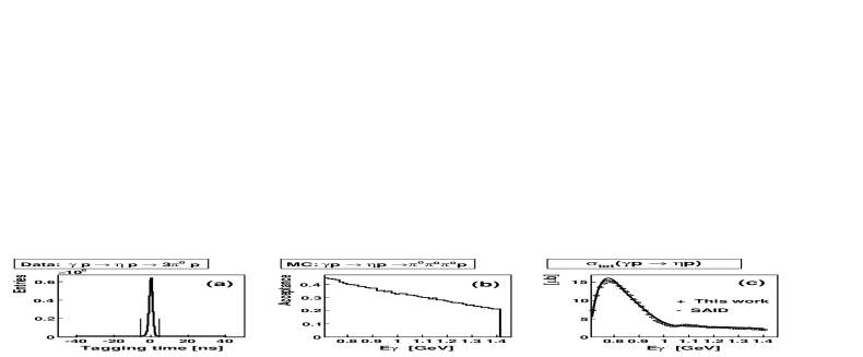
Figure 2: (a) Tagging-time distribution for the experimental $\eta\to 3\pi^{0}$ events, where the two vertical lines define the prompt region. (b) Acceptance for the $\eta\to 3\pi^{0}$ events as a function of the incident-photon energy. (c) Measured $\gamma p\to\eta p$ excitation function compared to the current PWA-fit solution from the SAID SAID data base.

The determination of the energy-resolution function $\Delta E/E$ for the CB and TAPS was divided into two steps. First, we fixed a so-called inherent resolution of the calorimeters, which is determined only by the propagation of electromagnetic showers in the GEANT simulation and by the cluster-reconstruction algorithm. The inherent energy resolution is better than the experimental one, which also includes additional smearing from the light collection, the conversion to electronic signals in the PMTs (photomultiplier tubes), digitization in the ADCs, and pileups. To match the experimental resolution, which is correlated with the beam intensity and depends on the quality of the gain calibrations, the MC output for the energy deposited in the calorimeters has to be smeared according to an “additional” $\Delta E/E$ function, which is different for different experimental conditions. For example, to match the experimental energy resolution for electromagnetic showers in the CB at a low intensity of the photon beam (i.e., with few pileups), the energy of clusters in the analysis of the MC simulation must be smeared according to $\Delta E/E=0.0145/(E[\mathrm{GeV}])^{0.34}$. Matching the energy resolution between the experimental and MC events can be adjusted via reaching agreement in the invariant-mass resolution and in the kinematic-fit stretch functions (or pulls) for the energy of the photons detected in the CB and TAPS. The superposition of the inherent and additional resolution functions is used in the kinematic-fit analysis of both the experimental data and MC simulation. This resolution function provides the uncertainties in the energy of the photon clusters. The functions parameterizing the energy resolution for electromagnetic showers in the CB and TAPS calorimeter are given in the section describing the experimental setup.

For seven-cluster events, the information from the recoil-proton cluster is also used in the kinematic fit. However, in contrast to the treatment of a photon cluster, the energy of the proton cluster is not included in the fit, as there is a large uncertainty in the loss of kinetic energy of the protons when they travel from the target to the calorimeter crystals. This loss occurs in the material located between the target and the crystal surface. The calculation of the kinetic energy of the protons from the cluster energies is complicated, as the amount of the material depends on the production angles in the laboratory system, and the energy loss in matter depends on the kinetic energy of the protons. Moreover, when the kinetic energy is above 450 MeV for the CB and above 370 MeV for TAPS, the recoil protons do not stop inside the crystals. In the analysis of six-cluster events, all parameters of the recoil proton (i.e., the kinetic energy and the two angles of the momentum vector) are free variables of the kinematic fit. The kinematic fitting includes the four main constraints, which are based on the conservation of energy and three-momentum, and additional constraints on the invariant masses of certain particles in the final state. For our reaction, we can use three constraints on the invariant mass of two photons to have the $\pi^{0}$-meson mass and a constraint on the invariant mass of six photons to have the $\eta$-meson mass. Then the total number of constraints to test the hypothesis of reaction (4) is eight. The effective number of constraints is smaller by the number of free variables of the fit, which are the $Z$ coordinate of the vertex and the unknown proton parameters (one for seven-cluster events and three for six-cluster events). Thus the test of hypothesis (4) is a 4-C (four effective constraints) fit for six-cluster events and a 6-C fit for seven-cluster events.

Note that testing the $\gamma p\to\eta p\to 3\pi^{0}p\to 6\gamma p$ hypothesis means testing this for all possible permutations of pairing the six photon clusters to form three $\pi^{0}$s. For six-cluster events, there are 15 such permutations. In the case of seven-cluster events, this number is seven times larger, as the proton cluster is also involved in the permutations. The number of permutations can be decreased by the separation of the photon clusters from the proton one. In our analysis, we used a limit on the $\theta$ angle of clusters, which can be only forward ones for the outgoing proton, and the information on the time of flight between a TAPS cluster and the CB signal with respect to the energy of the TAPS cluster. The time-of-flight information was also used to remove a small background from the six-cluster events, in which one of the clusters was due to the proton. The events for which at least one pairing combination satisfied the hypothesis of reaction (4) at the 2% confidence level, CL, (i.e., with a probability greater than 2%) were accepted as $\eta\to 3\pi^{0}$ event candidates. The pairing combination with the largest CL was used to reconstruct the kinematics of the reaction. A tighter cut on the kinematic-fit CL is unnecessary as there is almost no physical background to suppress. A looser cut on the CL is not desirable because of inclusion of events with poor resolution.

For the experimental events, in which there are usually several tagger hits recorded for one DAQ trigger, the $\gamma p\to\eta p\to 3\pi^{0}p\to 6\gamma p$ hypothesis is tested for every incident photon for which the tagging time is within a chosen interval and with the incident-photon energy above the reaction threshold of 707 MeV. If an $\eta\to 3\pi^{0}$ event candidate from one trigger passes the 2% CL criterion for several tagger hits, they are analyzed as separate events. The tagging-time spectrum for the experimental events selected as $\eta\to 3\pi^{0}$ candidates is shown in Fig. 2(a). The prompt peak from the coincidence of the DAQ triggers and the tagged photons sits above a uniform random background. All the experimental spectra were produced from the events where the tagging time lay between the vertical lines shown in Fig. 2(a), but are corrected for the random background by subtraction of the spectra produced from the events where the tagging time lay outside the prompt region. To decrease the statistical uncertainties and fluctuations in the experimental spectra obtained after the random-background subtraction, the width of the random region was taken to be much wider than the prompt one. The normalization factor for the subtraction of the random-background spectra is then the ratio of the widths taken for the prompt and the random parts of the spectrum.

Another source of background comes from interactions of the incident photons with the target walls. This background was investigated by analyzing the data taken with an empty target. The size of the so-called “empty-target” background depends on the thickness of the target walls and on how well the $\eta\to 3\pi^{0}$ production on hydrogen can be separated from production on heavier nuclei. Since the kinematic fit tests the hypothesis of the photon-proton interaction, this rejects many $\eta\to 3\pi^{0}$ events produced in the target walls. From our analysis, the size of the empty-target background in our $\eta\to 3\pi^{0}$ events is 2.2% after applying a cut at the 2% CL of the kinematic fit. Tightening this cut to the 10% CL decreases this background to 1.7%. Another way to suppress the empty-target background is to require the detection of the final-state proton. In this case, the empty-target background in our $\eta\to 3\pi^{0}$ events is 0.8% after applying a cut on the 2% CL and 0.65% for the 10% CL The corresponding numbers for our experimental $\eta\to 3\pi^{0}$ events with the undetected proton are 7.4% for the 2% CL and 6.0% for the 10% CL Because of limited statistics of the empty-target data, the remaining empty-target background was not subtracted from our experimental $\eta\to 3\pi^{0}$ spectra. The results obtained for the slope parameter $\alpha$ by the change in the size of the remaining empty-target background showed no dependence on it.

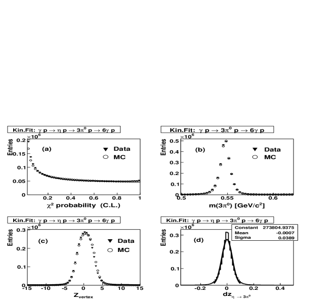
Figure 3: (a) The $\chi^{2}$ probability (or CL) distribution for the experimental (triangles) and MC (circles) $\eta\to 3\pi^{0}$ events; (b) the $3\pi^{0}$ invariant mass for the experimental (triangles) and MC (circles) $\eta\to 3\pi^{0}$ events selected at the 2% CL by testing the $\gamma p\to 3\pi^{0}p\to 6\gamma p$ hypothesis; (c) the $Z$ coordinate of the vertex for the experimental (triangles) and MC (circles) $\eta\to 3\pi^{0}$ events; (d) the resolution in the variable $z$.

The MC simulation of the $\gamma p\to\eta p\to 3\pi^{0}p$ reaction was divided into two steps. First, this reaction was simulated without dependence of its yield on the incident-photon energy. This MC simulation was used to determine the $\gamma p\to\eta p$ excitation function. Since we analyze the $\gamma p\to\eta p\to 3\pi^{0}p$ reaction at a large range of incident-photon energies, where the production angular distribution changes much, an isotropic distribution was used as an input for our MC simulation. The simulation of the $\eta\to 3\pi^{0}$ decay was made according to phase space (i.e., with the slope parameter $\alpha=0$). All MC events were propagated through a full GEANT (version 3.21) simulation of the CB-TAPS detector, folded with resolutions of the detectors (such as smearing according to the “additional” $\Delta E/E$ function) and conditions of the trigger, and analyzed in the same way as the experimental data. The resulting detector acceptance for the $\gamma p\to\eta p\to 3\pi^{0}p$ events selected by the kinematic fit at the 2% CL is shown in Fig. 2(b); it varies from about 45% at the $\eta$ threshold to about 25% at an incident-photon energy of 1.4 GeV. The experimental yield of the $\gamma p\to\eta p\to 3\pi^{0}p$ events corrected for the acceptance, for the $\eta\to 3\pi^{0}$ branching ratio, for the photon beam flux, and for the number of the target protons is compared in Fig. 2(c) to the current PWA-fit solution taken from the SAID SAID data base. The shape of the $\gamma p\to\eta p$ excitation function at the production threshold confirms the good quality of the energy calibration of the tagger, which was performed as explained in Ref. Tagger2 . The small disagreement that is seen at higher energies can be partially due to the difference between the real production angular distribution and the isotropic distribution used in our MC simulation. In the second step, the $\gamma p\to\eta p\to 3\pi^{0}p$ reaction was simulated according to its excitation function folded with the bremsstrahlung photon distribution. This MC simulation was then used to determine the slope parameter $\alpha$.

Since the event selection in our analysis is based on the confidence level of the kinematic fit, it requires good agreement of the $\chi^{2}$ probability (same as CL) distribution for the experimental and MC events. Then a change in the cut on the CL value removes the same fraction of events from the experimental data and MC simulation. In Fig. 3(a), we compare the CL distributions for the experimental (triangles) and MC (circles) events selected by testing the $\gamma p\to\eta p\to 3\pi^{0}p\to 6\gamma p$ hypothesis. These distributions are in reasonable agreement. Note that some increase in the CL distributions for low probability is due to events with partially overlapping photon showers, or with some leakage of the energy of the showers from the edge crystals of the CB and TAPS. Since the energy-resolution functions for the CB and TAPS were determined for “solitary” electromagnetic showers, for which all energy is deposited in the calorimeter, the errors in the energy and angles are underestimated for these “nonideal” clusters.

The agreement between the experimental data and MC simulation for the energy calibration of the calorimeters and the invariant-mass resolution can be illustrated by a comparison of the $3\pi^{0}$ invariant-mass spectra. These spectra obtained from events selected by testing the $\gamma p\to 3\pi^{0}p\to 6\gamma p$ hypothesis are shown in Fig. 3(b) by triangles for the experimental data and by circles for the MC simulation. There is good agreement between the experimental and MC spectrum for the mean value, which is consistent with the $\eta$-meson mass of 547.5 MeV, and for the invariant-mass resolution, which has $\sigma\approx 6$ MeV.

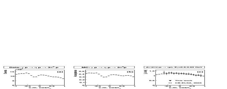
Figure 4: The angular distribution in the center-of-mass (c.m.) system for $\eta$ photoproduction in the $\gamma p\to\eta p$ reaction for incident-photon energies of 800 to 850 MeV: (a) measured distribution for the $\gamma p\to\eta p\to 3\pi^{0}p$ events, not yet corrected for the detector acceptance; (b) detector acceptance for the $\gamma p\to\eta p\to 3\pi^{0}p$ events; (c) our $\gamma p\to\eta p$ differential cross sections (triangles) compared to the CB-ELSA data CB-ELSA (circles).

Since the $Z$ coordinate of the vertex is a free variable in the kinematic fit, the $Z$ distribution must reflect the thickness of the LH₂ target, which is 5 cm long, and the target position. The agreement of these distributions for the experimental (triangles) and MC (circles) $\eta\to 3\pi^{0}$ events can be seen in Fig. 3(c). The larger width of the $Z$ distribution, compared to the 5-cm thickness of the physical target, is due to the resolution of the kinematic fit in the $Z$ coordinate. For the $\gamma p\to\eta p\to 3\pi^{0}p\to 6\gamma p$ process, this resolution is about 1.1 cm; it is determined from the difference between the initial and reconstructed value of $Z$ in the MC simulation.

Figure 5: Same as Fig. 4 but for incident-photon energies of 1150 to 1200 MeV.

The resolution in the variable $z$, defined in Eq.(3), can be understood from a comparison of $z$ calculated from the kinematics of the initially simulated events and $z$ calculated from the kinematics reconstructed for these events by the kinematic fit. The resolution in $z$ is shown in Fig. 3(d). Based on this resolution and the $z$-variable limits, which are from 0 to 1, we divided our $z$ spectra, used for the determination of the slope parameter, into 20 bins. This binning provides a bin width that is wider than one $\sigma_{z}=0.039$. The spectrum shown in Fig. 3(d) also demonstrates the insignificance of the combinatorial background in $\eta\to 3\pi^{0}\to 6\gamma$ events (i.e., when the kinematic-fit hypothesis with the largest CL chooses a false pairing combination of the six photons to the three $\pi^{0}$s). The combinatorial background produces accidental reconstructed values for $z$ that are spread widely in the $dz$ spectrum, resulting in a washout of the real Dalitz-plot slope. For a rough estimate of the combinatorial-background contribution, we took the fraction of the MC events that have $|dz|>0.2$; this fraction was found to be 3.5% only.

To show that our MC simulation satisfactorily reproduces the experimental acceptance, we compare our differential cross sections for the $\gamma p\to\eta p$ reaction with other existing measurements. In Fig. 4(a), we show the experimental distribution of the $\eta$ production angle from $\gamma p\to\eta p\to 3\pi^{0}p$ events measured in the center-of-mass (c.m.) system for incident-photon energies of 800 to 850 MeV. This distribution is not yet corrected for the acceptance. The corresponding acceptance obtained from our MC simulation is shown in Fig. 4(b). The complicated behavior of both the experimental distribution and the acceptance is mostly caused by the gap between the CB and TAPS calorimeters. The experimental distribution corrected for the acceptance, for the $\eta\to 3\pi^{0}$ branching ratio, for the photon beam flux, and for the number of the target protons is shown by triangles in Fig. 4(c). This distribution has a smooth shape now, which is in good agreement with the $\gamma p\to\eta p$ differential cross section obtained recently for the same energy range by the Crystal Barrel Collaboration at ELSA (CB-ELSA) CB-ELSA . The CB-ELSA data are shown by circles in the same figure. Similarly good agreement with the corresponding CB-ELSA results is observed for all other energy intervals. In Fig. 5, we illustrate it just for one more energy interval of 1150 to 1200 MeV. The agreement in the differential cross sections is shown to demonstrate the quality of our $\eta\to 3\pi^{0}$ analysis.

IV Determination of the slope parameter $\alpha$ and its uncertainty

The experimental $z$ distribution obtained for the $\eta\to 3\pi^{0}$ events with prompt tagging times is shown as the solid line in Fig. 6(a).

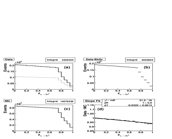
Figure 6: The $z$ distribution for the $\eta\to 3\pi^{0}$ events selected at CL=2% by testing the $\gamma p\to\eta p\to 3\pi^{0}p\to 6\gamma p$ hypothesis: (a) experimental prompt (solid line) and unnormalized random (dashed line) data; (b) experimental data after the subtraction of the normalized random background; (c) MC simulation for $4\times 10^{7}$ $\gamma p\to\eta p\to 3\pi^{0}p$ events; (d) the ratio of the experimental and MC distributions fitted to the function $p_{0}+2p_{1}z$.

The events were selected at the 2% CL from the test of the $\gamma p\to\eta p\to 3\pi^{0}p\to 6\gamma p$ hypothesis with the kinematic fit. Both six- and seven-cluster events (i.e., without and with the outgoing proton detected) were included in this distribution; the fraction of six-cluster events is only about 20%. The corresponding (unnormalized) $z$ distribution obtained from the events with the random tagging times is shown in the same figure by the dashed line. The size of this background depends on the photon-beam intensity and is less than 10% for our data. The experimental $z$ distribution after subtraction of the normalized random background is shown in Fig. 6(b). The $z$ distribution obtained from our MC simulation is shown in Fig. 6(c). This MC simulation is based on $4\times 10^{7}$ $\gamma p\to\eta p\to 3\pi^{0}p$ events with $\eta$ decaying to $3\pi^{0}$ according to phase space (i.e., with $\alpha=0$). The ratio of the experimental $z$ distribution to the MC one that was fitted to the function $p_{0}+2p_{1}z$ is shown in Fig. 6(d). To bring this fit to the required function $1+2\alpha z$, the MC distribution was normalized in such a way as to make the fit parameter $p_{0}$ equal to 1. Then the fit parameter $p_{1}=-0.0322\pm 0.0012$ has the meaning of the slope parameter $\alpha$. We take the error of $p_{1}$ from this fit, in which our full set of experimental statistics was used, as the statistical uncertainty of the slope parameter $\alpha$. To estimate its systematic uncertainty, a variety of tests were performed; these are listed in Table 1.

For each test listed in Table 1, we include information on the criteria for event selection, the experimental statistics, the value for the slope parameter with its statistical uncertainty, and the $\chi^{2}$/ndf value of the fit. The result of the fit shown in Fig. 6(d) is listed in Table 1 as test #1. Tests #2—#4 check the sensitivity of the results to the cut on the CL of the kinematic fit. Tightening the cut on the CL results in a data set with better resolution and less remaining background. The variation in the value for $\alpha$ is much smaller than the statistical uncertainties.

Tests #5—#7 check the sensitivity of the results to a possible background from the $3\pi^{0}$ final state that is not due to $\eta$ decay. The size of this background can be understood from the examination of the $3\pi^{0}$ invariant-mass spectrum obtained when testing the $\gamma p\to 3\pi^{0}p$ hypothesis. This spectrum is shown in Fig. 7 for the full tagging range 0.7—1.4 GeV of incident-photon energies and for the ranges 0.7—1.1 GeV and 1.1—1.4 GeV. An examination of the spectrum shows that the size of the $3\pi^{0}$ background comprises a few percent of our full data set, and it is negligibly small for events with the incident-photon energies below 1.1 GeV. We tested three cuts on the incident-photon energy: 0.9, 1.0, and 1.1 GeV. The experimental value for $\alpha$ is almost independent of this cut.

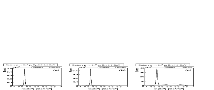
Figure 7: Experimental spectra for the $3\pi^{0}$ invariant mass obtained by testing the $\gamma p\to 3\pi^{0}p\to 6\gamma p$ hypothesis at the 2% CL for (a) the full tagging range of the incident-photon energies, $E_{g}=0.7-1.4$ GeV, (b) $E_{g}=0.7-1.1$ GeV, and (c) $E_{g}=1.1-1.4$ GeV.

Tests #8 and #9 check whether the simulation of the threshold on the CB total energy in the DAQ trigger is correct. From the analysis of the sum of the cluster energies, the parameters of the trigger were determined to be 320 MeV for the threshold itself and $\sigma=20$ MeV for its uncertainty. To reproduce these trigger conditions in the MC analysis, the total energy of clusters has be smeared according to a normal distribution having that $\sigma$, and those events that have a smeared energy less than the threshold value must be rejected from the analysis. In our tests, we applied software thresholds of 420 and 470 MeV to both the experimental and MC events. These magnitudes were chosen to be considerably larger than the threshold of 320 MeV smeared with $\sigma=20$ MeV. The results obtained for $\alpha$ are in good agreement within their statistical uncertainties.

Tests #10 and #11 check the sensitivity of our results to the difference between the isotropic production angular distribution used in the MC simulation of the $\gamma p\to\eta p$ reaction and the real distributions defined by the differential cross sections, which depend on the incident-photon energy. Examples of the $\gamma p\to\eta p$ differential cross sections for the two different intervals of the incident-photon energy are shown in Figs. 4 and 5. In these tests, we determined the slope parameter from two subsets. The first subset included the events with only $\cos\theta_{\eta}>0$ and the second one with only $\cos\theta_{\eta}<0$. Both the results for $\alpha$ are in agreement within their statistical uncertainties.

In tests #12—#17, we repeated some of the previous tests but for the seven-cluster events only. The results obtained are in good agreement with each other and with the tests that were performed using the sum of the events with both the cluster multiplicities.

Tests #18—#20 are performed for the six-cluster events only. The results for $\alpha$ are slightly smaller here in comparison to the corresponding seven-cluster results. This could be in part due to a larger fraction of the empty-target background in the six-cluster events. The $\eta\to 3\pi^{0}$ decay kinematics for this background is smeared by the kinematic fit, which assumes the target to be a proton. This smearing leads to poorer resolution in the variable $z$ and increases the combinatorial background, which reduces the real slope of the $\eta\to 3\pi^{0}$ Dalitz plot. A similar smearing occurs for the $\eta\to 3\pi^{0}$ events with accidental incident-photon energies (i.e., our random-background events). Test #21, in which $\alpha$ is obtained from the $\eta\to 3\pi^{0}$ events with accidental incident photons, illustrates the reduction in the experimental slope caused by the smearing effect. Differently from the empty-target background, the random background was subtracted in all tests of Table 1, except test #21.

Tests #22—#24 illustrate the stability of the results over the period of data taking. Our data set includes three periods of data taking from April 2007 to July 2007 with similar experimental and trigger conditions but different durations. All three results are in good agreement within their statistical uncertainties.

Table 1: Results for the $\eta\to 3\pi^{0}$ slope parameter $\alpha$ for different selection criteria

Result #	Cuts	Statistics	$\alpha$	$\chi^{2}$/ndf
1	CL=2%	$3.06\times 10^{6}$	$-0.0322\pm 0.0012$	31.5/18
2	CL=5%	$2.78\times 10^{6}$	$-0.0326\pm 0.0013$	32.2/18
3	CL=10%	$2.50\times 10^{6}$	$-0.0329\pm 0.0014$	30.0/18
4	CL=20%	$2.11\times 10^{6}$	$-0.0326\pm 0.0015$	25.9/18
5	CL=2%, $E_{\gamma}<1.1$ GeV	$2.76\times 10^{6}$	$-0.0320\pm 0.0013$	26.9/18
6	CL=2%, $E_{\gamma}<1.0$ GeV	$2.58\times 10^{6}$	$-0.0320\pm 0.0013$	28.9/18
7	CL=2%, $E_{\gamma}<0.9$ GeV	$2.18\times 10^{6}$	$-0.0321\pm 0.0015$	20.2/18
8	CL=2%, $E_{\mathrm{CB}}<0.42$ GeV	$2.83\times 10^{6}$	$-0.0316\pm 0.0013$	29.1/18
9	CL=2%, $E_{\mathrm{CB}}<0.47$ GeV	$2.60\times 10^{6}$	$-0.0319\pm 0.0013$	30.7/18
10	CL=2%, c.m. $\cos\theta_{\eta}<0.$	$1.73\times 10^{6}$	$-0.0334\pm 0.0017$	23.7/18
11	CL=2%, c.m. $\cos\theta_{\eta}>0.$	$1.32\times 10^{6}$	$-0.0312\pm 0.0019$	14.5/18
12	CL=2%, 7 cl.	$2.39\times 10^{6}$	$-0.0323\pm 0.0014$	26.4/18
13	CL=10%, 7 cl.	$1.97\times 10^{6}$	$-0.0327\pm 0.0015$	27.8/18
14	CL=20%, 7 cl.	$1.67\times 10^{6}$	$-0.0325\pm 0.0016$	26.9/18
15	CL=2%, 7 cl., $E_{\gamma}<1.1$ GeV	$2.13\times 10^{6}$	$-0.0319\pm 0.0015$	25.9/18
16	CL=2%, 7 cl., $E_{\gamma}<1.0$ GeV	$1.97\times 10^{6}$	$-0.0319\pm 0.0015$	28.5/18
17	CL=2%, 7 cl., $E_{\gamma}<0.9$ GeV	$1.62\times 10^{6}$	$-0.0323\pm 0.0017$	23.4/18
18	CL=2%, 6 cl.	$0.663\times 10^{6}$	$-0.0292\pm 0.0027$	22.0/18
19	CL=10%, 6 cl.	$0.525\times 10^{6}$	$-0.0307\pm 0.0030$	29.3/18
20	CL=20%, 6 cl.	$0.433\times 10^{6}$	$-0.0301\pm 0.0033$	25.4/18
21	CL=2%, random BkGr	$1.73\times 10^{6}$	$-0.0132\pm 0.0016$	23.2/18
22	CL=2%,  04.2007	$0.617\times 10^{6}$	$-0.0308\pm 0.0026$	21.0/18
23	CL=2%,  06.2007	$1.50\times 10^{6}$	$-0.0324\pm 0.0017$	23.6/18
24	CL=2%,  07.2007	$0.939\times 10^{6}$	$-0.0329\pm 0.0021$	16.8/18

The uncertainty in measuring the parameter $\alpha$ due to our limited resolution in the variable $z$ and the combinatorial background can be estimated by introducing the measured $\alpha$ value into the MC simulation and using this MC sample instead of the experimental data. To exclude statistical fluctuations from this estimate, the same MC sample must be used in the ratio of the simulations with nonzero and zero $\alpha$. This can be done when an event enters into the $z$ spectrum according to the $z$ value that is reconstructed by our program but with a weight of $1+2\alpha z$, calculated by using $z$ from the simulated kinematics of the event. In this way, the ideal $z$ distributions are folded with the experimental acceptance and resolution, and both spectra that are used in the ratio have correlated statistical fluctuations. These fluctuations are canceled in the ratio and do not smear the magnitude of the slope. The use of $\alpha=-0.032$ as an input for this estimate resulted in $\alpha=-0.0300\pm 0.0007$ after applying the criteria of test #1 and $\alpha=-0.0303\pm 0.0009$ after applying the criteria of test #4. The difference 0.0017 between the input $\alpha$ and the value obtained for $\alpha$ using the criteria of test #4 is slightly smaller than the value obtained using the criteria of test #1. This is expected because of a tighter quality cut on the CL of the kinematic fit in test #4. In the analysis of the MC simulation, we can also decrease the combinatorial background by applying an additional cut on the difference between the initially simulated and reconstructed value of $z$. The elimination of the MC events that have $|dz|>0.2$, additionally to the selection criteria of test #1, results in $\alpha=-0.0315\pm 0.0007$, which is in good agreement with $\alpha=-0.032$ used as an input. These tests illustrate the importance of the experimental resolution for the precision measurement of the slope parameter $\alpha$.

As our final result for the slope parameter $\alpha$, we use the weighted average of all results from Table 1 except tests #18—#21, which were performed for the six-cluster events and the random background. The six-cluster results are omitted as they involve larger background and much poorer statistics. The weight factor of each result was taken as the inverse value of its statistical uncertainty. This procedure gives $-0.0322$ for the value of $\alpha$. Note that this value is identical to the result for $\alpha$ obtained from test #1, which is based on our full experimental statistics and could be considered as an alternative choice of our main value for $\alpha$. For the statistical uncertainty of $\alpha$, we take the uncertainty 0.0012 from our full-statistics test #1. In the systematic uncertainty of $\alpha$, we include half of the largest variation of the results in Table 1 (except tests #18—#21), which is 0.0013, and 0.0017 obtained earlier as the difference between the initially simulated $\alpha=-0.032$ and the reconstructed value for $\alpha$. Adding these uncertainties in quadrature gives 0.0022 for our total systematic uncertainty.

An uncertainty in the parameter $\alpha$ resulting from a possible cusp in the $\pi^{0}\pi^{0}$ invariant-mass spectrum is found to be insignificant. The details on the cusp search are given in the next section.

The value $\alpha=-0.0322\pm 0.0012_{\mathrm{stat}}\pm 0.0022_{\mathrm{syst}}=-0.0322\pm 0.0025_{\mathrm{tot}}$, obtained in our measurement for the $\eta\to 3\pi^{0}$ slope parameter , is in good agreement with the PDG value for $\alpha$, which is $-0.031\pm 0.004$ PDG , but it has a smaller uncertainty. That the present PDG value for $\alpha$ is identical to the result of the Crystal Ball at the AGS eta_slope_bnl means that the new Crystal Ball Collaboration at MAMI confirms the previous measurement. Finally, taking into account the magnitude of our total uncertainty, we prefer to give the rounded value

$$\alpha=-0.032\pm 0.003_{\mathrm{tot}}$$ (5)

as our final value for the slope parameter.

V Search for a cusp structure in the $\pi^{0}\pi^{0}$ invariant-mass spectrum

Figure 8: The ratio of the experimental spectrum for the $\pi^{0}\pi^{0}$ invariant mass to the corresponding MC spectrum is shown by crosses for (a) the phase-space decay of $\eta\to 3\pi^{0}$ in the MC simulation (i.e., with $\alpha=0$) and for (b) the MC simulation of the $\eta\to 3\pi^{0}$ decay with $\alpha=-0.032$ . The ratio of the MC simulation with $\alpha=-0.032$ to the MC simulation with $\alpha=0$ is shown in (a) by dots. The corresponding ratios of the MC spectra with two versions of the cusp prediction are shown by dashed (using Ref. Belina ) and solid (using Ref. Bissegger ) lines in (a) for the case when $\alpha=-0.032$ and in (b) when $\alpha=0$.

The magnitudes of $\chi^{2}$/ndf for the fits from Table 1 hint that the linear hypothesis, $1+2\alpha z$, is not completely accurate for describing the slope of the experimental $\eta\to 3\pi^{0}$ Dalitz plot. A possible explanation could be the occurrence of a cusp effect in the $\pi^{0}\pi^{0}$ invariant-mass spectrum from the $\eta\to 3\pi^{0}$ decays. The origin of such a cusp was discussed in the Introduction. In this section, we check whether a cusplike structure is seen in our data and how its presence could affect our result for $\alpha$. Since the effect of the cusp in $\eta\to 3\pi^{0}$ is expected to be small, the most convenient distribution to see it is the ratio of the experimental and MC spectrum for the $\pi^{0}\pi^{0}$ invariant mass. This ratio is shown by crosses in Fig. 8(a) for the case where the MC simulation of the $\eta\to 3\pi^{0}$ decay is made according to phase space (i.e., with $\alpha=0$). Since the experimental $\pi^{0}\pi^{0}$ invariant-mass spectrum is already distorted from phase space by the nonzero $\alpha$, we also show the ratio in which the MC simulation with $\alpha=-0.032$ is taken instead of the experimental data; it is shown by dots in the same figure. This ratio, for the most part, is in reasonable agreement with the experimental one. The largest deviation is seen around a mass of 0.28 GeV, which corresponds to the $\pi^{+}\pi^{-}$ threshold. To better separate the effect of the cusp from that of a nonzero $\alpha$ value, we replaced the phase-space MC simulation in the data-to-MC ratio by the MC simulation that includes the slope parameter $\alpha=-0.032$ for the $\eta\to 3\pi^{0}$ decay. The result of this replacement is shown by crosses in Fig. 8(b).

The magnitude of the cusplike structure, which is seen at the level of 1% only, is much smaller than the prediction made in Ref. Belina (shown by a dashed curve in Fig. 8). The shape and the sign of the cusplike structure also look different. For a more correct comparison, each theoretical prediction shown in the figures is folded with our experimental resolution. Because of the smallness of the effect observed in the $\pi^{0}\pi^{0}$ invariant-mass spectrum, better statistics is desirable to draw any final conclusion on the magnitude and features of the cusp.

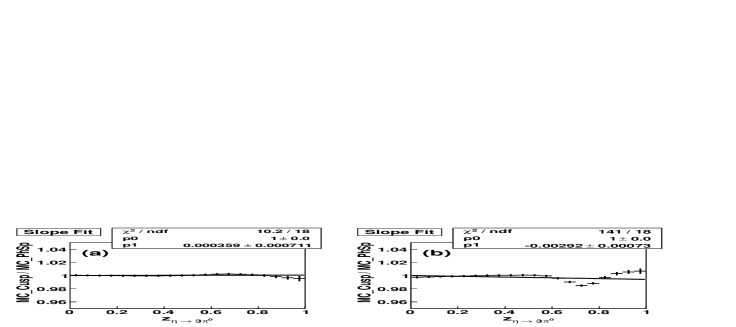
Figure 9: Ratio of $z$ distributions (crosses) for the $\eta\to 3\pi^{0}$ decays simulated with and without a cusp: (a) corresponds to the solid curve and (b) to the dashed curve in Fig. 8(b). The solid lines show fits to the function $p_{0}+2p_{1}z$.

Trying to reach a closer agreement between the data and a model prediction, we used formulas from Ref. Bissegger . The authors of this article conduct a detailed theoretical study of cusps in $K_{L}\to 3\pi$ decays and also indicate the way to use their approach in the $\eta\to 3\pi$ case if one starts from the following parametrization of the decay tree amplitudes: $A(\eta\to 3\pi^{0})=u_{0}+u_{1}z$ and $A(\eta\to\pi^{+}\pi^{-}\pi^{0})=v_{0}+v_{1}y+v_{2}y^{2}+v_{2}x^{2}$ with the conventional $\eta\to 3\pi$ Dalitz plot variables. The cusp shape in $\eta\to 3\pi^{0}$ then depends strongly on the parameters of the $\eta\to\pi^{+}\pi^{-}\pi^{0}$ tree amplitude, which are still not well determined. To use the parameters available from analyses of the density distribution of the $\eta\to 3\pi$ Dalitz plots, we assumed that $|A(\eta\to 3\pi^{0})|^{2}\sim 1+2(u_{1}/u_{0})z=1+2\alpha z$ and $|A(\eta\to\pi^{+}\pi^{-}\pi^{0})|^{2}\sim 1+2(v_{1}/v_{0})y+(2v_{2}/v_{0}+v_{1}^{2}/v_{0}^{2})y^{2}+2(v_{3}/v_{0})x^{2}=1+ay+by^{2}+cx^{2}$. It turned out that, after some variation of the $\eta\to\pi^{+}\pi^{-}\pi^{0}$ parameters ($a$, $b$, and $c$), by starting from the ones that are available in the PDG PDG , the agreement of the cusp prediction with the data can be improved. An example of such an improvement is shown by the solid curve in Fig. 8. Further improvement requires a simultaneous fit of the $\eta\to 3\pi^{0}$ and $\eta\to\pi^{+}\pi^{-}\pi^{0}$ data, which is not the topic of this paper. The current agreement is sufficient to understand our systematic uncertainty in the parameter $\alpha$ resulting from a possible cusp at the $\pi^{+}\pi^{-}$ threshold. In Fig. 9, we illustrate the deviation of the slope in the $z$ distribution from the phase space for the two cusp shapes that were shown in Fig. 8. As shown, if the cusp structure is similar to the one that is consistent with our data, then the effect of the cusp on the $\eta\to 3\pi^{0}$ slope is negligible. However, the cusp as predicted in Ref. Belina would cause significant distortion away from the linear behavior; this is not observed in our experimental data.

VI Summary and conclusions

The dynamics of the $\eta\to 3\pi^{0}$ decay have been studied with the Crystal Ball multiphoton spectrometer and the TAPS calorimeter. Bremsstrahlung photons produced by the 1.5-GeV electron beam of the Mainz Microtron MAMI-C and tagged by the Glasgow photon spectrometer were used for $\eta$-meson production. The analysis of $3\times 10^{6}$ $\gamma p\to\eta p\to 3\pi^{0}p\to 6\gamma p$ events yields the value $\alpha=-0.032\pm 0.003$ for the $\eta\to 3\pi^{0}$ slope parameter, which agrees with the majority of recent experimental results and has the smallest uncertainty. The agreement with $\alpha=-0.031\pm 0.004$ of the measurement made by the Crystal Ball at the AGS, where the $\pi^{-}p\to\eta n$ reaction was used, demonstrates the suitability of photoproduction for studying subtle effects in $\eta$ decays. The $\pi^{0}\pi^{0}$ invariant-mass spectrum was investigated for the occurrence of a cusplike structure in the vicinity of the $\pi^{+}\pi^{-}$ threshold. The observed effect is small and does not affect our measured value for the slope parameter. Further investigation of the cusp requires better statistics and a simultaneous analysis of $\eta\to 3\pi^{0}$ and $\eta\to\pi^{+}\pi^{-}\pi^{0}$ data.