Possible evidence for a common radial structure in nearby AGN tori

We present a quantitative and relatively model-independent way to assess the radial structure of nearby AGN tori. These putative tori have been studied with long-baseline infrared (IR) interferometry, but the spatial scales probed are different for different objects. They are at various distances and also have different physical sizes which apparently scale with the luminosity of the central engine. Here we look at interferometric visibilities as a function of spatial scales normalized by the size of the inner torus radius $R_{\rm in}$. This approximately eliminates luminosity and distance dependence and, thus, provides a way to uniformly view the visibilities observed for various objects and at different wavelengths. We can construct a composite visibility curve over a large range of spatial scales if different tori share a common radial structure. The currently available observations do suggest model-independently a common radial surface brightness distribution in the mid-IR that is roughly of a power-law form $r^{-2}$ as a function of radius $r$, and extends to $\sim$100 times $R_{\rm in}$. Taking into account the temperature decrease toward outer radii with a simple torus model, this corresponds to the radial surface density distribution of dusty material directly illuminated by the central engine roughly in the range between $r^{0}$ and $r^{-1}$. This should be tested with further data.

1 Introduction

Speckle and long-baseline interferometry in the infrared (IR) has started to explore the spatial structure of the putative tori in Active Galactic Nuclei (AGN; e.g. Wittkowski et al., 1998; Weinberger et al., 1999; Swain et al., 2003; Weigelt et al., 2004; Jaffe et al., 2004; Wittkowski et al., 2004; Meisenheimer et al., 2007; Tristram et al., 2007). However, the number of long baselines per object is still generally limited, and a given baseline probes different spatial scales for targets at various distances and having different physical sizes. Here we investigate the possibility of uniformly view these interferometric measurements taken for various objects spanning over different wavelengths, by studying them as a function of spatial scales in units of torus inner radius.

Table 1: List of AGNs used in this paper.

name	type	$cz^{a}$	obs. date	inst.	$\lambda$	$b$	PA	$R_{\rm in}$	K-band	reference	$\Delta$PAg
		(km s-1)	(UT)		($\mu$m)	(m)	($\deg$)	(mas)	Lag (days)		(deg)
NGC1068	2	914	2003-06-15/16	MIDI	8.2-13	79	-179	1.6b		Jaffe et al. (2004)	89
NGC1068	2	914	2003-11-09/10	MIDI	8.2-13	46	-135	1.6b		Jaffe et al. (2004)	45
Mrk1239	1	6321	2005-12-19	MIDI	8.2-13	41	36	0.17c		Tristram et al. (2008)	86
NGC3783	1	3234	2005-05-28	MIDI	8.2-13	43	46	0.32	85d	archive	0
NGC3783	1	3234	2005-05-31	MIDI	8.2-13	65	120	0.32	85d	Beckert et al. (2008)	74
NGC4151	1	1242	2003-05-23	KI	2.2	83	37	0.47	48e	Swain et al. (2003)	50

^aRadial velocity corrected for the cosmic microwave background from NED.
^bCalculated from the estimated intrinsic $V$-band flux (Pier et al., 1994) and Eq.3.
^cCalculated from the $V$-band flux $f_{\nu}=7.8$mJy (Véron-Cetty & Véron, 2003) and Eq.3.
^dGlass (1992). ^eMinezaki et al. (2004). ^fSuganuma et al. (2006).
^gPosition angle difference between the projected baseline and the expected torus major axis direction (see text).

2 Composite radial structure

2.1 Spatial frequency per inner torus radius

The radius $R_{\rm in}$ of the inner boundary of the torus dust distribution is thought to be set by dust sublimation. In this case, for a given sublimation temperature and grain size distribution, $R_{\rm in}$ is expected to be proportional to $L^{1/2}$, where $L$ is the UV/optical luminosity of the central engine (e.g. Barvainis, 1987). This propotionality was recently confirmed by Suganuma et al. (2006) through near-IR reverberation measurements. These provide the inner torus radius as the light travel distance for the time-lag between the variability in the optical and the near-IR. It is conceivable that the dust temperature structure within the torus is primarily determined by the illumination from the central source and is, thus, also expected to scale with $L^{1/2}$. In this case, if we view various interferometric size information as a function of spatial scales normalized by $R_{\rm in}$, at least the primary luminosity dependence of the data, as well as the distance dependence, is eliminated.

A direct observable in an interferometric measurement is the visibility, or the normalized Fourier amplitude of the brightness distribution of a source, as a function of spatial scales (or spatial wavelength; see below) given in angular size. Here we normalize the spatial scale by the angular size of $R_{\rm in}$. More precisely, the Fourier component is studied as a function of spatial frequency, i.e. the number of spatial cycles in a given angular size. Thus we study here visibilities as a function of the number of spatial cycles in $R_{\rm in}$, or spatial frequency per $R_{\rm in}$.

For a given projected baseline $b$ in m, observing wavelength $\lambda$ in $\mu$m, and $R_{\rm in}$ in milli-arcsecond (mas), the spatial freqency in cycles per $R_{\rm in}$, written here as $u\cdot R_{\rm in}$ (where $u$ is a spatial frequency per mas), is given as

$$u\cdot R_{\rm in}=4.85\times 10^{-3}\frac{b\ {\rm(m)}\ }{\lambda\ {\rm({\mu}m)}}\cdot R_{\rm in}\ {\rm(mas)}\ \ \ {\rm(cycles\ per}\ R_{\rm in}{\rm)}.$$ (1)

The corresponding spatial wavelength $\Lambda$, i.e. the reciprocal of spatial frequency $u$, is given in units of $R_{\rm in}$ as

$$\Lambda/R_{\rm in}=2.06\times 10^{2}\ \frac{\lambda\ {\rm({\mu}m)}}{b\ {\rm(m)}}\cdot\frac{1}{R_{\rm in}\ {\rm(mas)}}.$$ (2)

This corresponds to the representative spatial resolution of the configuration ($b$ and $\lambda$). For simple geometries, the visibility takes the first null at a spatial wavelength $\Lambda$ roughly equal to the characteristic size (e.g. diameter of an uniform disk or a ring). The quantity $\Lambda$ can also be compared directly to the diffraction limit of $2.5\times 10^{2}\ {\rm(mas)}\ \lambda{\rm({\mu}m)}/D{\rm(m)}$ for a single aperture diameter $D$. We will study visibilities as a function of these two quantities, $u\cdot R_{\rm in}$ and $\Lambda/R_{\rm in}$, throughout this paper.

An accurate scale length for the inner boundary radius $R_{\rm in}$ has not been well determined yet. As the most plausible, observationally motivated quantity, we adopt the one obtained from the near-IR reverberation time-lag radii, or, if not available, the overall fit to them as a function of UV/optical luminosity $L$ given by Suganuma et al. (2006). In the latter case, the angular size for the time-lag radius is given as a function of observed flux $f_{\nu}$ in $V$-band as (the same as Eq.4 in Kishimoto et al. 2007)

$$R_{\rm in}=0.43\ [f_{\nu}(V)\ /\ (50\ {\rm mJy})]^{1/2}\ {\rm(mas)}.$$ (3)

We note that the time-lag radius is actually a factor of $\sim$3 smaller, for a given luminosity $L$, than the sublimation radius given by Barvainis (1987) assuming graphite grains with radial size $a$=0.05 $\mu$m and sublimation temperature $T_{\rm sub}$=1500 K. The possible reasons for this difference have been discussed by Kishimoto et al. (2007), including the possibility that $R_{\rm in}$ is determined by much larger grains. As we discuss below, the reverberation radius is supported by the near-IR interferometry of NGC 4151 (Swain et al., 2003). The uncertainty in the time-lag radii is $\sim$0.2 dex, based on the scatter of the fit.

2.2 Data

The data most suitable for the radial structure study are those for Type 1 AGNs. In these objects, the tori are thought to have much smaller inclinations than in Type 2 AGNs, so that the radial structure can be studied without a significant orientation effect. We would also expect that the dependence on the exact PAs of the projected baselines is relatively small (the torus image projected on to the sky would not be far from being circular-symmetric; see more below). Those Type 1 objects for which long-baseline IR interferometric data are found in the literature or archive are listed in Table 1, along with the adopted size for $R_{\rm in}$. All the mid-IR data here were obtained with VLTI/MIDI. In addition, we also use the MIDI data for the Type 2 AGN NGC1068 of Jaffe et al. (2004). The data provide the highest spatial frequency information in the mid-IR, and the inclination effect at these wavelengths is expected to be relatively small compared with that in the near-IR (see more below).

All the MIDI data were uniformly re-reduced with the software EWS (version 1.5.2; Jaffe 2004), with a few modifications using our own IDL codes. First, since MIDI visibility measurements for the faint Type 1 targets ($\lesssim$ 1 Jy) are largely limited by the accuracy of photometric (total flux) measurements, we implemented an additional background subtraction for the photometry frames. Second, to reduce errors in group delay determinations, we have smoothed delay tracks over $\sim$10-20 frames. To avoid possible positive bias in correlated flux, we also averaged $\sim$10-20 frames for the determination of phase offsets.

The system visibility was obtained from the observations of visibility calibrators usually taken right after or before each target observation with a similar airmass. These data were also reduced with similar smoothings above to calibrate out the effect of the time averaging. These calibrators are also generally the photometric standards found in the list by Cohen et al. (1999). We obtained the correlated flux, which was corrected for the system visibility, and total flux separately. The errors for the total flux and correlated flux were estimated from the fluctuation of the measurements over time. For the targets with a few total flux measurements available, we took weighted means. The errors for the final visibilities were obtained from the estimated errors in the correlated flux and total flux (except for NGC1068 where the errors were estimated from the scatter of several available visibility measurements).

2.3 Mid-IR surface brightness distribution

Fig.1 shows the visibility data listed in Table 1 as a function of spatial frequency per $R_{\rm in}$ (or spatial wavelength $\Lambda$ in units of $R_{\rm in}$; upper $x$-axis). The $x$-axis is in log scale to cover a large range of spatial frequencies as given by different objects and by different observing wavelengths. The red/yellow/green colors correspond to wavelenths from 13 to 8.2 $\mu$m, while purple is for 2.2 $\mu$m. The MIDI data have been binned with $\Delta\lambda\sim 0.4$ $\mu$m, with the error for each bin taken as the median of the errors over the binned spectral channels (since errors over adjacent channels are correlated). For comparison, we plot the visibility curves for ring, gaussian, and power-law intensity distributions of different indices with an inner cut-off radius $R_{\rm in}$.

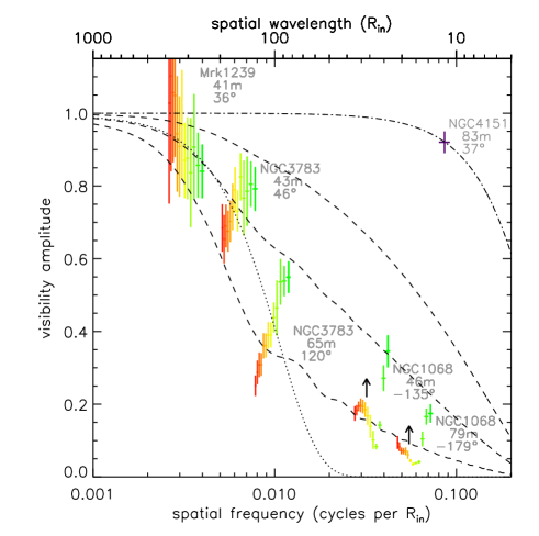
Figure 1: Observed visibilities as a function of spatial frequency per inner torus radius. The red/yellow/green colors correspond to from 13 to 8.2 $\mu$m and purple corresponds to 2.2 $\mu$m. The mid-IR data are binned with $\Delta\lambda\sim 0.4\mu$m. The arrows are to show that the NGC1068 data are taken as the lower limit for the visibilities of Type 1s at the same spatial frequencies. Visibility curves for various simple geometries are also plotted; three dashed curves, power-law with index -2.5, -2.0, and -1.5 from top to bottom; dotted, Gaussian with HWHM 25 $R_{\rm in}$; dot-dashed, ring with radius $R_{\rm in}$.

At a given observing wavelength, as the torus inclination increases from face-on to edge-on cases (i.e. from Type 1 to Type 2 inclinations), the visibilities are expected to generally decrease, since the inner bright radiation becomes obscured and this effectively makes the overall size of the intensity distribution larger. (Here we are restricting our discussion to the spatial frequencies within the first lobe, i.e. those less than the one at which the visibility reaches the first null.) On the other hand, this decrease is expected to be quite small at long wavelengths, such as in the mid-IR, due to much smaller obscuration effects. Therefore, the mid-IR visibilities of the Type 2 AGN NGC1068 provide quite a meaningful lower limit for those of the Type 1 objects at the same spatial frequencies (indicated by the upward arrows in Fig.1).

If we put together the lower limit from NGC1068 with the visibilities observed for the Type 1 AGNs in the mid-IR (Fig.1), the data at different spatial freqencies appear quite coherent, i.e. consistent with the case where these objects share roughly a common radial brightness distribution in face-on inclinations. When compared with various model curves shown in Fig.1, the mid-IR brightness distribution appears to be consistent with a power-law form, where the index is $\sim-2$ at $\sim$8 $\mu$m.

The visibility functions for power-law distributions shown in Fig.1 are for the cases with the outer cut-off radius $R_{\rm out}=100R_{\rm in}$. For the power-law distributions with index $\geq-2$, $R_{\rm out}$ changes the shape of visibility functions, especially at low spatial frequencies. Here, the data at high spatial frequencies (NGC1068 and the longer baseline data for NGC3783) roughly fix the power law index. Then the low spatial frequency data further constrain $R_{\rm out}$, which corresponds to the outer radius of the mid-IR emission region, to be roughly $\sim$100$R_{\rm in}$ (see also section 3).

In order to be least sensitive to the possible dependency of the visibilities on the position angle (PA) of the projected baseline, we would ideally want to compare the visibilities of each object as well as different objects measured at the major axis direction of the torus projected on to the sky. The minor axis PA can be estimated from a linear radio jet structure ($\sim$77° for NGC4151, Mundell et al. 2003; $\sim$0° for NGC1068, e.g. Gallimore et al. 2004) or optical polarization PA ($\sim$136° for NGC3783, Smith et al. 2002; $\sim$40° for Mrk1239, Goodrich 1989). The PA difference between the projected baseline and the expected major axis is listed in Table 1. Unfortunately, these relative PAs are not uniform for the data gathered here. However, they do not seem to disturb the composite visibility diagram shown in Fig.1, which might indicate that the PA dependence is small as we expect and assumed here for Type 1s. Further data are needed to address this issue. The two data sets for the Type 2 object NGC1068 have quite different PAs, which is probably adequate for obtaining lower limits for Type 1 visibilities.

The only existing near-IR measurement for Type 1 AGNs, i.e. the one for NGC 4151 (Fig.1, purple cross), is consistent with a ring of radius $R_{\rm in}$. It is quite expected that the torus shows a much more compact structure in the near-IR than in the mid-IR, since the former reflects the distribution of materials at higher temperatures. For a given inner boundary radius $R_{\rm in}$, the ring model represents essentially the most compact structure, giving the upper limit for the visibilities. This essentially means that $R_{\rm in}$ generally cannot be much larger than assumed here (the observed data points would move to the right in Fig.1 if we adopt larger $R_{\rm in}$ for each object, which would exceed the upper limit given by the $R_{\rm in}$ ring). Future near-IR data at high spatial frequencies are crucial to settle this issue.

Note that we should in principle correct the observed visibility for the possible contribution from the unresolved accretion disk in the near-IR to estimate the intrinsic visibility of the torus alone. The correction depends on the estimate of the near-IR flux fraction from the disk, which in turn depends on the assumed near-IR spectral shape of the accretion disk. The correction, however, is estimated to be very small (less than 5% reduction; Kishimoto et al. 2007), as long as the disk spectrum is bluer than observed in the UV/optical which seems quite likely (e.g. Kishimoto et al. 2008).

All the visibility functions shown in Fig.1 reach the first null at a spatial wavelength $\Lambda\sim$ a few $R_{\rm in}$ (outside the figure) due to the inner boundary diameter being 2$R_{\rm in}$. In the mid-IR, detailed intensity distributions in the inner few $R_{\rm in}$ region will not affect the overall visibility curves significantly, since a major fraction of the mid-IR radiation originates from larger regions. To discuss whether the same model can account for both the mid-IR and near-IR data, we need a physical torus model.

3 Torus model

We aim here to generically describe the torus surface brightness distribution with as a few parameters as possible. In various torus models, two types of dust distributions have been considered; namely, smooth and clumpy distributions (e.g. Pier & Krolik, 1992, 1993; Granato & Danese, 1994; Efstathiou & Rowan-Robinson, 1995; Nenkova et al., 2002; Dullemond & van Bemmel, 2005; Schartmann et al., 2005; Hönig et al., 2006; Schartmann et al., 2008). We first consider the latter and assume that the torus consists of various discrete dust clouds each being optically thick. The constraints from the alternative case of smooth dust distribution will be considered later below.

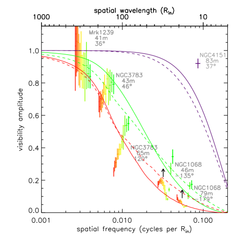
Figure 2: Observed visibilities as compared with physical torus models. Red/green/purple curves are for the observing wavelengh of 13/8.5/ 2.2 $\mu$m , respectively. Solid curves are with $\alpha=0.0$ for the $\gamma=0$ case, while dotted curves are with $\alpha=-0.9$ for the $\gamma=1.6$ case.

The near- and mid-IR torus radiation is primarily dominated by that from those clouds which are directly illuminated by the central engine (e.g. Hönig et al. 2006). We can then approximately parameterize the face-on surface brightness distribution $S_{\nu}(r)$ at an observing frequency $\nu$ as a function of radius $r$ as

$$S_{\nu}(r)=I_{\nu}(T_{\rm max}(r))\cdot(r/R_{\rm in})^{\alpha}.$$ (4)

The first term, $I_{\nu}$, is the intensity from an illuminated cloud as a function of $T_{\rm max}(r)$, which is the maximum temperature of the dust grains at radius $r$ written as

$$T_{\rm max}=T_{\rm sub}\cdot(r/R_{\rm in})^{-\frac{2}{4+\gamma}}.$$ (5)

This is derived from the thermal equilibrium of a dust grain and involves the wavelength dependency of the absorption efficiency of the grain in the form of its spectral index $\gamma$ in the infrared (Barvainis, 1987). For the large grain limit, $\gamma$=0, while for the standard interstellar material (ISM) dust grains, $\gamma\sim 1.6$. The sublimation temperature $T_{\rm sub}$ is taken here as 1500K, but our conclusions below are not sensitive to this exact value of $T_{\rm sub}$.

The specific intensity $I_{\nu}$ from an illuminated dust cloud needs to be obtained with a proper radiative transfer calculation, but is approximately of the form

$$I_{\nu}=\int e^{-\tau}B_{\nu}(T(\tau))\ d\tau$$ (6)

for an optically thick cloud, where $T(\tau)$ is the temperature of the dust grains at an optical depth $\tau$ from the surface of the cloud, and $B_{\nu}(T)$ is the Planck function. At a given observing frequency, however, we can assume that the intensity distribution over the torus radius, $I_{\nu}(r)$, approximately scales with $B_{\nu}(T_{\rm max}(r))$.

The second term in the expression for $S_{\nu}$, $(r/R_{\rm in})^{\alpha}$, describes the distribution of the normalized surface density, or the filling factor per unit area, of the illuminated material as a power law form. An implicit assumption here is that the dust cloud distribution in the innermost region is opaque so that $S_{\nu}(R_{\rm in})=I_{\nu}(T_{\rm sub})$, and this is the maximum brightness so that $\alpha\leq 0$.

In this way, we can model the visibilities as a function of the parameter $\alpha$ for an assumed dust grain size distribution fixed by $\gamma$. We consider the two cases above; namely, the large grain limit ($\gamma=0$) and the ISM case ($\gamma=1.6$). For each case, we can estimate an adequate density index $\alpha$ for roughly reproducing the visibilities observed in the 8-13 $\mu$m range. We show in Fig.2 such representative curves where $\alpha$ is taken to be 0.0 and -0.9 for the $\gamma=0$ and 1.6 cases, respectively. We estimate the uncertainties in these indices to be $\sim$0.3, based on the uncertainty in the visibility measurements and also in $R_{\rm in}$ ($\sim$0.2 dex; see sec. 2.1).

All the curves shown in Fig.2 have been calculated with an outer boundary of 100 $R_{\rm in}$. The results do not change significantly if a larger outer boundary is adopted (the region outside 100$R_{\rm in}$ contains only a small fractional amount in the mid-IR). Therefore, in the $100R_{\rm in}$ cases adopted here, the outer boundary is set almost by the temperature distribution, rather than the density distribution of the illuminated material.

Let us consider briefly the case of smooth dust distribution. If the opening angle of the geometrical distribution is constant over the radii, i.e. if there is no geometrical flaring, the material at large radii is illuminated only by the attenuated radiation from the central engine. Then $I_{\nu}$ would represent the intensity from the dust grains at radius $r$ where the distribution of the maximum temperature $T_{\rm max}(r)$ is steeper (decreasing more quickly with radius) than considered for the clumpy case above. Therefore, the normalized surface density distribution, $(r/R_{\rm in})^{\alpha}$, has to be shallower, closer to the upper limit of $\alpha=0$. If there is a geometrical flaring, then we would revert to consider the directly illuminated surface at each radius, leading to essentially the same conclusions obtained for the clumpy case.

As for the consistency with the near-IR data, the large grain case produces slightly more compact distributions in the near-IR than the ISM case (because the temperature distribution is steeper), and is marginally consistent with the NGC4151 data. Thus the large grain case is slightly favored here. We note that the large grain case is consistent with the small innermost radii suggested by the near-IR reverberations, though other contributing factors are not ruled out (Kishimoto et al., 2007). While we would need a more detailed modeling of the surface brightness distribution for the innermost region, we also need more observational data in the near-IR to constrain such detailed models.

4 Conclusions

The long-baseline IR interferometry data for AGN tori are still generally limited in $uv$ coverage for each target. The data for various objects probe different spatial scales. We argue that one way to uniformly study these various data is to view them as a function of spatial frequency per inner torus boundary radius $R_{\rm in}$, or spatial scale in units of $R_{\rm in}$. In this way, using primarily the data for Type 1 AGNs, we have tried to construct a composite visibility function over a wide range of spatial scales and investigated the radial structure of the tori. The data obtained so far suggest a common radial distribution of the face-on surface brightness in the mid-IR that is approximately of a power-low form with index $\sim-2$ and extends to $\sim$100$R_{\rm in}$. Considering the temperature distribution of the dust grains, this corresponds to the surface density distribution of the directly illuminated material ranging approximately between $r^{0}$ and $r^{-1}$. We aimed here to derive direct constraints with a simple model. Further data are definitely needed over the wavelengths from the near-IR to mid-IR to test the composite visibility function and to further constrain models.