Dynamics of interacting dark energy

Abstract

Dark energy and dark matter are only indirectly measured via their gravitational effects. It is possible that there is an exchange of energy within the dark sector, and this offers an interesting alternative approach to the coincidence problem. We consider two broad classes of interacting models where the energy exchange is a linear combination of the dark sector densities. The first class has been previously investigated, but we define new variables and find a new exact solution, which allows for a more direct, transparent and comprehensive analysis. The second class has not been investigated in general form before. We give general conditions on the parameters in both classes to avoid unphysical behavior (such as negative energy densities).

I Introduction

Cosmological observations point to the existence of non-baryonic cold matter and of a late-time acceleration of the universe (see, e.g. Dunkley et al. (2008); Tegmark et al. (2006); Percival et al. (2007)). If gravity is modelled on cosmological scales by general relativity, and if we assume that the universe is homogeneous and isotropic on these scales, then the late-time acceleration is sourced by a dark energy component, and the universe is dominated by the “dark sector”. The quest to uncover the true nature of dark matter (DM) and dark energy (DE) is one of the most pressing topics of modern cosmology.

One of the fundamental puzzles within this quest is the “coincidence problem”: how is it that we seem to live in a time when the densities of DM and DE are of the same order of magnitude, given that they evolve very differently with redshift? An interesting proposal is that interaction between the dark fields could perhaps alleviate the coincidence problem. Various interaction models have been put forward and studied (see, e.g. Wetterich (1995); Amendola (1999); Billyard and Coley (2000); Zimdahl and Pavon (2001); Dalal et al. (2001); Farrar and Peebles (2004); Chimento et al. (2003); Cai and Wang (2005); Majerotto et al. (2004); Nunes and Mota (2006); Olivares et al. (2005); Sadjadi and Alimohammadi (2006); Guo et al. (2007); Garcia-Compean et al. (2008); Setare and Vagenas (2007); Boehmer et al. (2008); Quartin et al. (2008); Quercellini et al. (2008); Valiviita et al. (2008); He et al. (2008); Chen et al. (2008)).

For a flat FRW universe, the background dynamics after recombination are governed by the equations of energy balance and the Raychaudhuri field equation:

$$\dot{\rho}_{b} = -3H\rho_{b}\,,$$ (1a)

$$\dot{\rho}_{c} = -3H\rho_{c}+Q\,,$$ (1b)

$$\dot{\rho}_{x} = -3(1+w_{x})H\rho_{x}-Q\,,$$ (1c)

$$\dot{H} = -4\pi G\left[\rho_{b}+\rho_{c}+(1+w_{x})\rho_{x}\right],$$ (1d)

where $H=\dot{a}/a$ is the Hubble parameter, $\rho_{c}$ is the cold DM density, $\rho_{b}$ is the baryonic density, $\rho_{x}$ is the density of DE and $w_{x}<0$ is its constant equation of state. The baryons only interact gravitationally with the dark sector, and $Q$ is the rate of energy transfer in the dark sector. The Friedmann constraint equation is

$$H^{2}=\frac{8\pi G}{3}\left(\rho_{b}+\rho_{c}+\rho_{x}\right)\,.$$ (2)

Note that the field equations (1d) and (2) are independent of $Q$, because of total energy conservation. A positive $Q>0$ represents transfer of energy from DE to DM; a negative $Q<0$ represents transfer of energy from DM to DE.

In this paper, we consider interactions that are linear combinations of the dark sector densities:

$$Q=A_{c}\rho_{c}+A_{x}\rho_{x}\,.$$ (3)

Here the rate factors $A_{I}$ are either proportional to $H$ or constants, leading to two classes of interaction model:

Model I $$A_{I}=3\alpha_{I}H\,,$$ (4)

Model II $$A_{I}=3\Gamma_{I}\,,$$ (5)

where $\alpha_{I}$ are dimensionless constants and $\Gamma_{I}$ are constant transfer rates. Observations impose the general constraint that the interaction should be sub-dominant today, so that

$$|\alpha_{I}|\ll 1\,,~{}~{}~{}~{}|\Gamma_{I}|\ll H_{0}\,.$$ (6)

Model I has been recently analysed by Quartin et al. (2008) (and earlier work considered the special cases $\alpha_{c}=\alpha_{x}$ Chimento et al. (2003) and $\alpha_{x}=0$ Billyard and Coley (2000)). We use an alternative approach, defining new variables to simplify the parameter space, and finding the general exact solution. We are able to recover previous results more directly and simply, and to provide some new insights into the model.

The $H$ in the $Q$-term for Model I is motivated purely by mathematical simplicity. By contrast, the energy exchange in Model II is motivated by similar models that have been used in reheating Turner (1983), curvaton decay Malik et al. (2003) and decay of DM to radiation Cen (2000). As far as we know, Model II for the dark sector interaction has has not been treated in the general case before. The special case $\Gamma_{x}=0$ has been analyzed by Valiviita et al. (2008) (and by Boehmer et al. (2008) in the case where DE is modelled by exponential quintessence).

A summary of the paper is as follows. Some properties of the general case ($Q$ not specified) are presented in Sec. II. Model I is studied in Sec. III. In Sec. IV, we analyze Model II. Finally, we conclude in Sec. V.

II The case of general $Q$

We define the dimensionless dynamical variablesCopeland et al. (1998)

$$x=\frac{8\pi G}{3H^{2}}\rho_{x}\,,\quad y=\frac{8\pi G}{3H^{2}}\rho_{c}\,,\quad z=\frac{8\pi G}{3H^{3}}Q\,.$$ (7)

Before proceeding further, we now show that we can “hide” the constant DE equation of state by defining a new interaction variable $\tilde{z}:=z/(-w_{x})$; in this way, all our results below will be independent of the value of $w_{x}$.

The dark sector balance equations read

$$x^{\prime} = 3x\left(1-x\right)-\tilde{z}\,,~{}~{}\tilde{z}:=-\frac{z}{w_{x}}\,,$$ (8a)

$$y^{\prime} = -3xy+\tilde{z}\,,$$ (8b)

where a prime denotes $d/d(-w_{x}N)$, with $N=\ln a$ (we choose $a_{0}=1$). The baryonic density is determined by the Friedmann constraint,

$$\frac{8\pi G}{3H^{2}}\rho_{b}=1-x-y\,.$$ (9)

We cannot solve the system of equations until $Q$ is specified, but we can draw some conclusions for a general $Q$ or $\tilde{z}$. The simplest cases are $\tilde{z}=\tilde{z}(x,y)$, when the system (8) is closed and autonomous. Model I is such a case. The next simplest cases are those for which $z$ is not determined algebraically by $x$ and $y$, but does satisfy an equation of motion of the form $\tilde{z}^{\prime}=F(x,y,\tilde{z})$, so that we have a 3-dimensional autonomous system. Model II is an example of this case.

The critical points $(x_{*},y_{*})$ of the dynamical system (8) must comply with the conditions

$$3x_{*}\left(1-x_{*}-y_{*}\right)=0\,,$$ (10a)

$$-3x_{*}\left(1-x_{*}+y_{*}\right)+2\tilde{z}_{*}=0\,,$$ (10b)

where $\tilde{z}_{*}$ is the interaction variable $\tilde{z}$ evaluated at the critical points. Equation (10a) implies that either $x_{*}=0$, which represents the usual matter dominated point, or $x_{*}+y_{*}=1$, which implies no contribution from the baryonic component.

From Eq. (10b), we see that the option $x_{*}=0$ directly implies that $\tilde{z}_{*}=0$. Thus pure matter domination can only exist if the interaction term vanishes at the corresponding point. On the other hand, the option $x_{*}+y_{*}=1$ leads to

$$3x_{*}(1-x_{*})=\tilde{z}_{*}\,.$$ (11)

If the dynamical system is autonomous, the above equation depends only on $x_{*}$ and gives the position of the critical point that is compatible with a nonzero interaction term (and no baryonic contribution). By contrast, if the system is not autonomous, we require extra information before we can completely determine its critical points.

Another quantity of interest is the dark energy-to-dark matter (DE-DM) ratio, $R=\rho_{x}/\rho_{c}$. From Eqs. (8) we obtain the evolution equation

$$\frac{R^{\prime}}{R}=3-\frac{(x+y)}{xy}\tilde{z}\,,~{}~{}R=\frac{\rho_{x}}{\rho_{c}}=\frac{x}{y}\,,$$ (12)

which is equivalent to Eq. (3) in del Campo et al. (2008, 2009). As we show below, this equation can lead to exact solutions in some particular models. A key point relates to the factor $(x+y)$ in Eq. (12): its substitution by the Friedmann constraint (9) in some cases can hide the existence of exact solutions (e.g. Barrow and Clifton (2006); Quartin et al. (2008); del Campo et al. (2008, 2009)). The standard non-interacting case, $\tilde{z}=0$, shows the expected exponential result $R=R_{0}e^{-3w_{x}N}$, where $R_{0}=\Omega_{x0}/\Omega_{c0}\sim 3.4$ is the present value of the DE-DM ratio.

If the current value of $R$ is close to an asymptotic value, $R_{0}\simeq R_{\infty}:=R(\infty)$, then the coincidence problem is “solved”. (Strictly, one has transferred the coincidence problem to a problem of explaining the dark sector interaction.) In this case, $R$ must be a slowly-evolving function as $N\to\infty$, i.e. $R^{\prime}\simeq 0$ at late times, which requires

$$3xy-\tilde{z}\left(x+y\right)\simeq 0\,.$$ (13)

As we shall discuss below, for some models this condition is met only at some points of the phase-space.

III Model I: $Q=3H\left(\alpha_{x}\rho_{x}+\alpha_{c}\rho_{c}\right)$

This model was intensively studied in Quartin et al. (2008) (our $\alpha_{I}$ correspond to their $\lambda_{I}$). We find the critical points in a more direct way, and also find the general exact solution. This allows us to recover many of their results more directly and simply, and to provide some new insights into the model.

III.1 Critical points and their properties

The dimensionless interaction variable $\tilde{z}$ is

$$\tilde{z}=3\left(\tilde{\alpha}_{x}x+\tilde{\alpha}_{c}y\right)\,,~{}~{}\tilde{\alpha}_{I}=-\frac{\alpha_{I}}{w_{x}}\,.$$ (14)

Thus $\tilde{z}=\tilde{z}(x,y)$ and the phase-space is 2-dimensional and autonomous.

As discussed before, the first type of critical point in Eqs. (10) is that for which $x_{*}=0$ and $\tilde{z}_{*}=0$. Such a critical point in the present model also needs $y_{*}=0$, and then it corresponds to a baryon dominated point. This point is not realistic and we will exclude it from our analysis; for more details, see Quartin et al. (2008).

The critical points that are compatible with a non-zero interaction term comply with the constraint $x_{*}+y_{*}=1$ and are solutions of Eq. (11) in the form

$$x_{*}\left(1-x_{*}\right)=\tilde{\alpha}_{x}x_{*}+\tilde{\alpha}_{c}\left(1-x_{*}\right)\,.$$ (15)

The critical points and their linear stability are summarized in Table I; the results are in agreement with those of Quartin et al. (2008). For convenience we have defined the parameters

$$C_{1} = \frac{1}{2}\left(1-\tilde{\alpha}_{x}-\tilde{\alpha}_{c}\right)\,,$$ (16a)

$$C_{2} = \sqrt{C^{2}_{1}-\tilde{\alpha}_{x}\tilde{\alpha}_{c}}\,.$$ (16b)

Note that the existence condition for the critical points ensures that $C_{2}$ is real.

Point	$x_{*}$	$y_{*}$	Existence	Eigenvalues	Stability
					Unstable if $x_{A}<0$ and $C_{2}+\alpha_{x}>0$
A	$C_{1}+\tilde{\alpha}_{c}-C_{2}$	$1-x_{A}$	$C^{2}_{2}\geq 0$	$-3(C_{1}+\tilde{\alpha}_{c}-C_{2})$;	Saddle if $x_{A}>0$ and $C_{2}+\alpha_{x}>0$
				$6(C_{2}+\tilde{\alpha}_{x})$	or: $x_{A}<0$ and $C_{2}+\alpha_{x}<0$
					Stable if $x_{A}>0$ and $C_{2}+\alpha_{x}<0$
B	$C_{1}+\tilde{\alpha}_{c}+C_{2}$	$1-x_{B}$	$C^{2}_{2}>0$	$-3(C_{1}+\tilde{\alpha}_{c}+C_{2})$;	Saddle if $x_{B}<0$
				$-6C_{2}$	Stable if $x_{B}>0$

Table 1: Critical points of Model I and their stability. $C_{1},C_{2}$ are given in Eqs. (16); notice that $C_{2}$ is positive by definition. The existence conditions are given here in general, but the discussion in the text suggests that both interaction parameters should be positive, see Eq. (20), so that both $x_{A}$ and $x_{B}$ are positive too. Thus, point A is of the saddle type whereas point B is stable.

For a physically viable model, one of the critical points should correspond to a DM dominated universe, $x\to 0$ and $y\to 1$, at early enough times; moreover, this critical point should be an unstable point. The only candidate is point A, but $x_{A}\neq 0$. For DM domination we need $|x_{A}|\ll 1$; to linear order in $x_{*}$, we obtain from Eq. (15) that

$$x_{A}\simeq\frac{\tilde{\alpha}_{c}}{1-\tilde{\alpha}_{x}}\,,\quad y_{A}\simeq\frac{2C_{1}}{1-\tilde{\alpha}_{x}}\,.$$ (17)

At late times we must get a DE dominated universe, which should correspond to the stable point B. For the latter, Eq. (15) gives the estimate

$$x_{B}\simeq\frac{2C_{1}}{1-\tilde{\alpha}_{c}}\,,\quad y_{B}\simeq\frac{\tilde{\alpha}_{x}}{1-\tilde{\alpha}_{c}}\,.$$ (18)

For certain parameter values the DE density is negative at early times Quartin et al. (2008) (see also Valiviita et al. (2008) in the cases $\alpha_{x}=0$ and $\alpha_{x}=\alpha_{c}$). In a first approximation we can use Eqs. (17) and (18) to determine the conditions under which both DM and DE are non-negative and well behaved at all times.

At early times, we must impose the constraint

$$0\leq x_{A}\simeq\frac{\tilde{\alpha_{c}}}{1-\tilde{\alpha}_{x}}<1\,,.$$ (19)

which is satisfied if

$$\tilde{\alpha}_{c}\geq 0\,,\quad 1>\tilde{\alpha}_{x}+\tilde{\alpha}_{c}\,,$$ (20)

or

$$\tilde{\alpha}_{c}\leq 0\,,\quad 1<\tilde{\alpha}_{x}+\tilde{\alpha}_{c}\,.$$ (21)

Likewise, at late times we have the constraint

$$0\leq y_{B}\simeq\frac{\tilde{\alpha}_{x}}{1-\tilde{\alpha}_{c}}<1\,,$$ (22)

and then the same conditions (20) and (21) apply, but now with the interaction constants interchanged, $\tilde{\alpha}_{c}\leftrightarrow\tilde{\alpha}_{x}$. It can be verified that the conditions described above give the correct description for the different cases depicted in Figs. 7, 8 and 9 in Quartin et al. (2008).

It follows that for a plausible scenario, the interaction parameters $\tilde{\alpha}_{c}$ and $\tilde{\alpha}_{x}$ must be both non-positive or both non-negative. A remarkable result arises now. If the interaction parameters are to have the same sign, the only permitted case is that of Eq. (20), as the case in Eq. (21) cannot be consistently satisfied if the interaction parameters are both negative.

Another constraint appears from the condition that the critical points are such that $0\leq x_{*},y_{*}\leq 1$. From Eqs. (17), we get $\tilde{\alpha}_{x}<1$; likewise, from Eqs. (18) we get $\tilde{\alpha}_{c}<1$. Finally, the critical points should be real, $C^{2}_{2}\geq 0$, and then the allowed values $(\tilde{\alpha}_{c},\tilde{\alpha}_{x})$ are those located below the rotated parabola

$$(\tilde{\alpha}_{x}-\tilde{\alpha}_{c})^{2}\geq 2(\tilde{\alpha}_{x}+\tilde{\alpha}_{c})-1\,.$$ (23)

Therefore, we arrive at the overall conclusion that $0\leq\tilde{\alpha}_{c}\,,\tilde{\alpha}_{x}\leq 1$ if the DM and DE contributions are to be positive and well behaved, $0<x,y<1$, at all times. This is in agreement with the results of Quartin et al. (2008) (see the critical points $A_{2}$ and $B_{2}$ in Table I). We used a first order calculation based on Eqs. (17) and (18); however, by continuity, we expect the result to be true even in cases where DE and DM contribute significantly at early and late times.

A more general statement exists regarding the positivity of the dark components at early times. Note that we can write Eq. (15) for the critical points in the form

$$3w_{x}x_{*}y_{*}=-3\left(\alpha_{x}x_{*}+\alpha_{c}y_{*}\right)=-z_{*}\,.$$ (24)

If both DM and DE are to be positive for all times, then $z$ and $w_{x}$ should have opposite signs. This explains why the DE component becomes negative at early times in certain models: it is because the interaction variable $z$ can become negative at DM domination. In our case, non-negative interaction constants ensure that both DM and DE are positive at all times (see also Figs. 7 and 9 in Quartin et al. (2008) for some other examples.)

In Fig. 1, we show the allowed values of the interaction parameters (represented by the red shaded region) according to the discussion above.

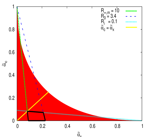
Figure 1: The red shaded region contains the allowed non-negative values of $\tilde{\alpha}_{c}$ and $\tilde{\alpha}_{x}$ satisfying the reality constraint (23). The cyan (dotted) line represents the equality in Eq. (34) for $R_{i}=0.1$, the blue (dashed) line represents the equality in Eq. (36) for $R_{0}=3.4$, and the green (dashed-dotted) line is Eq. (37) with $R_{\infty,m}=10$. The yellow (solid) line corresponds to the particular case $\alpha_{c}=\alpha_{x}$ Chimento et al. (2003). The only region that provides reasonable values of the DE-DM ratio at both early and late times is the one surrounded by the thick black (solid) lines. The value $R_{i}=0.1$ was chosen for presentation purposes; the allowed region would become much smaller for a more realistic value $R_{i}\ll 0.1$.

III.2 DE-DM ratio: exact solution

With the interaction term (14), Eq. (12) becomes

$$R^{\prime}=-3\left[\tilde{\alpha}_{x}R^{2}-\left(1-\tilde{\alpha}_{x}-\tilde{\alpha}_{c}\right)R+\tilde{\alpha}_{c}\right]\,.$$ (25)

This equation provides the known solutions of simpler cases, e.g. for the case $\alpha_{x}=0$, we have

$$R=\left(\frac{\Omega_{x0}}{\Omega_{c0}}+\frac{\alpha_{c}}{w_{x}+\alpha_{c}}\right)e^{-3(w_{x}+\alpha_{c})N}-\frac{\alpha_{c}}{w_{x}+\alpha_{c}}\,,$$ (26)

which directly recovers Eq. (7) of Guo et al. (2007). Here we present the new solution in the general case $\alpha_{x}\neq 0$:

$$R(N)=\frac{C_{1}}{\tilde{\alpha}_{x}}-\frac{C_{2}}{\tilde{\alpha}_{x}}\tanh\left[3w_{x}C_{2}\left(N-N_{1}\right)\right]\,,$$ (27)

where $C_{1}$ and $C_{2}$ are given by Eqs. (16), and the integration constant is

$$N_{1}=-\frac{1}{3w_{x}C_{2}}\tanh^{-1}\left[\frac{1}{C_{2}}\left(\tilde{\alpha}_{x}\,\frac{\Omega_{x0}}{\Omega_{c0}}-C_{1}\right)\right]\,.$$ (28)

Using Eq. (27) we can integrate the DM energy balance equation to obtain the DM density as a function of $N$:

$$\rho_{c}=\rho_{c0}e^{(-3-\alpha_{c}-C_{1})N}\left[\frac{\cosh 3C_{2}(N-N_{1})}{\cosh 3C_{2}N_{1}}\right]^{1/3},$$ (29)

and then the DE density follows directly as $\rho_{x}(N)=R(N)\rho_{c}(N)$.

The asymptotic values of the DE-DM ratio from Eq. (27) are directly related to the values inferred from the critical points in Table 1,

$$R_{-\infty} := R(-\infty)=\frac{C_{1}-C_{2}}{\tilde{\alpha}_{x}}=\frac{x_{A}}{y_{A}}\,,$$ (30a)

$$R_{\infty} := R(\infty)=\frac{C_{1}+C_{2}}{\tilde{\alpha}_{x}}=\frac{x_{B}}{y_{B}}\,.$$ (30b)

It follows that the smallest value of the DE-DM ratio $R_{-\infty}$ is determined by the critical point A; likewise, its largest value $R_{\infty}$ is determined by the critical point B. The correspondence between the asymptotic values of $R$ and the critical points A and B is not surprising after all, because the roots of $R^{\prime}=0$ in Eq. (25) are actually the ratios inferred from the critical points.

There is an interesting point concerning the initial values of the DE-DM ratio. For given values of the free parameters of the model ($w_{x}$, $\alpha_{x}$, and $\alpha_{c}$), the initial value of the DE-DM ratio, $R_{i}$, should be such that

$$R_{i}>R_{-\infty}\,,$$ (31)

otherwise the evolution of the DE-DM ratio is not described by Eq. (27). A similar constraint exists for the late time value $R_{\infty}$:

$$R_{\infty}>R_{0}\,,$$ (32)

to ensure that the value $R_{0}$ is included in the range of values allowed by the exact solution (27).

Further constraints on the values of the interaction parameters can be obtained from Eqs. (31) and (32). According to Eq. (17), if the DE contribution is to be small at early times, we can write

$$R_{-\infty}=\frac{x_{A}}{y_{A}}\simeq\frac{\tilde{\alpha}_{c}}{2C_{1}}\,,$$ (33)

and then, for a given value of $R_{i}$, Eq. (31) becomes the constraint

$$\tilde{\alpha}_{c}<\frac{R_{i}}{1+R_{i}}(1-\tilde{\alpha}_{x})\,.$$ (34)

By using Eq. (18), i.e. under the assumption that the DM contribution is small at late times, we find the companion expression of Eq. (33), which is

$$R_{\infty}=\frac{x_{B}}{y_{B}}\simeq\frac{2C_{1}}{\tilde{\alpha}_{x}}\,,$$ (35)

and then Eq. (32) becomes the constraint

$$\tilde{\alpha}_{c}<1-(1+R_{0})\,\tilde{\alpha}_{x}\,.$$ (36)

If we want an upper limit on $R_{\infty}$, i.e. $R_{\infty}<R_{\infty,m}$, where $R_{\infty,m}$ is some maximum value, then a new constraint arises from Eq. (35),

$$\tilde{\alpha}_{c}>1-(1+R_{\infty,m})\,\tilde{\alpha}_{x}\,.$$ (37)

The inclusion of the constraint equations (34), (36), and (37) in Fig. 1 indicates that only a small region of the parameter space may be compatible with observations. The examples in Fig. 1 correspond to $R_{i}=0.1$, $R_{0}=3.4$ and $R_{\infty,m}=10$.

It can be verified that the above results are in agreement with the results presented in Quartin et al. (2008); Chimento et al. (2003); Guo et al. (2007); Valiviita et al. (2008); Olivares et al. (2008); Barrow and Clifton (2006). In particular, the diverse cases presented in those papers are explained in a unified way by the exact solution (27), and our approach provides very simple expressions for the analysis of the parameter space. For example, it readily explains the troublesome features encountered in Figs. 7, 8 and 9 of Quartin et al. (2008).

In Fig. 2 we show examples of the evolution of the DE-DM ratio for fixed values $R_{\infty}$, $R_{0}$, and $w_{x}$. The curves correspond to different values of $\tilde{\alpha}_{x}$, and the values of $\tilde{\alpha}_{c}$ were determined from Eq. (35). Finally, we show in Fig. 3 a typical example of a phase space with parameters in the allowed region of Fig. 1.

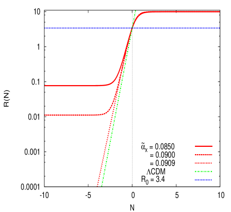
Figure 2: Evolution of the DE-DM ratio $R(N)$ according to Eqs. (27) and (16). The chosen values of the various parameters are $R_{0}=3.4$, $R_{\infty}=10$, whereas the value of $\tilde{\alpha}_{c}$ was determined from Eq. (35) for the given values of $\tilde{\alpha}_{x}$. For comparison, the green (dashed-dotted) line represents the standard $\Lambda$CDM case. The dotted line corresponds to exactly $\tilde{\alpha}_{c}=0$, for which case $R_{-\infty}=0$ and the earlier evolution is very similar to that of standard $\Lambda$CDM.

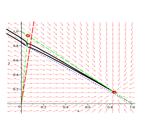
Figure 3: The phase space of Model I in the case $\tilde{\alpha}_{x}=0.15$, and $\tilde{\alpha}_{c}=0.05$. The (red) circles are the critical points A and B (see Table 1), and the green dashed line is the (heteroclinic) constraint $x+y=1$ that connects them. The green dot-dashed line that connects the saddle point A to the unstable critical point at the origin is a good approximation to the heteroclinic trajectory between the two points. The red long-dashed line represents the ratio $x/y=0.1$. The blue dotted line is the approximate Friedmann constraint (39). The black (solid) lines are numerical solutions of the equations of motion for different initial conditions. The trajectories with initial conditions on the right of the heteroclinic line end up at point B; if the initial conditions are on the left, the DE component becomes negative and the DM one grows without bound.

We are assuming that the initial conditions are set at the onset of matter domination, and that the DM to baryonic matter ratio is the same as in the standard case,

$$\left.\frac{\rho_{b}}{\rho_{c}}\right|_{i}\simeq\frac{\Omega_{b,0}}{\Omega_{m,0}}\simeq\frac{1}{5}\,.$$ (38)

Note that the above is just an approximation, since the DM component in the interacting case does not evolve exactly as $a^{-3}$, see Eq. (29). Then the initial conditions of the DM and DE contributions, with the help of the Friedmann constraint (9), are determined from

$$x_{i}+\frac{6}{5}y_{i}\simeq 1\,.$$ (39)

Some examples of numerical solutions of the equations of motion are shown in Fig. 3 for different initial conditions. All of them represent valid solutions that start at a matter dominated epoch and end in a final state with finite DE-DM ratio. This final state is uniquely determined by the values of the free parameters of the model.

The phase space portrait reveals some other aspects of the interacting model under consideration, apart from the critical points and their stability studied above. It shows the line $R_{-\infty}=x/y$, which approximates very well the heteroclinic curve that connects the (unstable) critical point at the origin (actually, this is the baryonic dominated critical point discussed in Sec. III.1) with the (saddle) point A. It is then apparent that any curve with initial DE-DM ratio $R_{i}<R_{-\infty}$ leads to trajectories in which the DE component is negative and the DM grows without bound.

Therefore, the constraint equation (31) is not only necessary for the trajectory to be described in terms of the DE-DM ratio in Eq. (27), but it is also needed to have a reasonable evolution of the universe after the onset of matter domination.

The initial value $R_{i}$ is related to the e-fold number $N_{i}$ by

$$R_{i}=-\frac{C_{1}}{\alpha_{x}}+\frac{C_{2}}{\alpha_{x}}\tanh\left[3C_{2}\left(N_{i}-N_{1}\right)\right]\,,$$ (40)

where $N_{1}$ is determined from Eq. (28), so that there is a one-to-one correspondence between $R_{i}$ and $N_{i}$. Thus different initial conditions result in different times for the appearance of a matter dominated epoch. Different initial conditions can have dramatic effects on the past history of the universe, even if the final state can be arranged to be the same in all cases.

III.3 Special cases

Our results apply for some special cases already present in the literature. For instance, if $\tilde{\alpha}_{x}=\tilde{\alpha}_{c}$Chimento et al. (2003), then Eqs. (16) suggest that $\tilde{\alpha}_{c}\leq 1/4$ for the critical points to be real (see also Eq. (23)). Moreover, Eq. (17) implies that $\tilde{\alpha}_{c}\ll 1$ if proper matter domination is to appear and then $R_{A}\ll 1$. Since Eqs. (19) and (22) together imply that $R_{B}=1/R_{A}$, this model has difficulty to achieve an asymptotically constant DE-DM ratio relevant to the coincidence problem.

Another example is $\tilde{\alpha}_{x}=0$ Guo et al. (2007), for which the critical points, from Eq. (15), are $x_{A}=\tilde{\alpha}_{c}$ and $x_{B}=1$. However, Fig. 1 indicates that any reasonable model necessarily needs $\tilde{\alpha}_{x}\neq 0$ to alleviate the coincidence problem.

For completeness, we can also have the case $\tilde{\alpha}_{c}=0$. Then there is proper matter domination for any value $0\leq\tilde{\alpha}_{x}\leq 1$, because $x_{A}=0$, and the case is free from the problems related to a finite value of $R_{-\infty}$, see Figs. 1, 2, and 3. The coincidence problem can be addressed if the only non-zero interaction parameter is given an appropriately small value, as $R_{B}\simeq 1/\tilde{\alpha}_{x}$.

IV Model II. $Q=3\left(\Gamma_{x}\rho_{x}+\Gamma_{c}\rho_{c}\right)$

In the simplest model of the reheating process after inflation in the early universe, one assumes that the oscillating inflaton field $\phi$ behaves like a matter fluid that decays into relativistic particles; the decay is parametrized by a constant decay width $\Gamma_{\phi}$ Turner (1983). In our notation, $Q=\Gamma_{\phi}\rho_{\phi}$. Motivated by this, and by similar models for curvaton decay Malik et al. (2003) and for decay of DM to radiation Cen (2000), we arrive at Model II: $Q=3(\Gamma_{x}\rho_{x}+\Gamma_{c}\rho_{c})$, where the $\Gamma_{I}$ are constant decay widths. Unlike Model I, the $Q$ here is not constructed a priori for mathematical simplicity, and the dynamics are considerably more complicated as a result.

The variable $z$ becomes

$$z=3\left(\frac{\Gamma_{x}}{H}x+\frac{\Gamma_{c}}{H}y\right)\,,$$ (41)

which typically grows in an expanding universe, and diverges in the limit $H\to 0$. Because of this, it is convenient to define the new variable Boehmer et al. (2008),

$$u:=\frac{H_{0}}{H+H_{0}}\,,$$ (42)

which allows us to compactify the evolution of $z$. Here, $H_{0}$ denotes the current value of the Hubble parameter. Early times correspond to $u\to 0$, and late times to $u\to\rm{const}$ (if $\dot{H}<0$, then $u\to 1$). As in Model I, we redefine the interaction variables as

$$\tilde{\alpha}_{I}(u):=\frac{u}{1-u}\frac{\gamma_{I}}{(-w_{x})}\,,\quad\gamma_{I}:=\frac{\Gamma_{I}}{H_{0}}\,.$$ (43)

Notice that $u_{0}=1/2$ and then $\tilde{\alpha}_{I0}=\gamma_{I}/(-w_{x})$. Thus

$$\tilde{z}=\frac{3u}{1-u}\frac{(\gamma_{x}x+\gamma_{c}y)}{(-w_{x})}=3\left[\tilde{\alpha}_{x}(u)\,x+\tilde{\alpha}_{c}(u)\,y\right]\,,$$ (44)

which is a time-dependent version of the Model I expression (14). The equations of motion become

$$x^{\prime} = 3x\left(1-x\right)-3\left[\tilde{\alpha}_{x}(u)\,x+\tilde{\alpha}_{c}(u)\,y\right]\,,$$ (45a)

$$y^{\prime} = -3xy+3\left[\tilde{\alpha}_{x}(u)\,x+\tilde{\alpha}_{c}(u)\,y\right]\,,$$ (45b)

$$u^{\prime} = -\frac{3}{2w_{x}}(1+w_{x}x)u(1-u)\,,$$ (45c)

where a prime again denotes $d/d(-w_{x}N)$. Note that the DE equation of state appears explicitly in Eq. (45c) because the value of $w_{x}$ is necessary to know the time evolution of the cosmological model.

IV.1 Critical points

The system (45) is autonomous, and, to begin with, Eq. (45c) admits the critical values $u_{*}=0$ and $u_{*}=1$.

If $u_{*}=0$, then Eqs. (45a) and (45b) suggest the critical values: (a) $x_{*}=0$, with $y_{*}$ to be determined from the Friedmann constraint (9); and (b) $x_{*}=1$ and $y_{*}=0$. These are the expected critical points from the general discussion in Sec. II, see Eqs. (10). The stability of these points can be established by standard methods, from which we find that (a) is unstable, while (b) is of saddle type for $-1<w_{x}<0$ and stable for $w_{x}<-1$.

Point	$x_{*}$	$y_{*}$	$u_{*}$	Existence	Eigenvalues	Stability
A	$0$	$y_{*}$	$0$	all $\gamma_{c}\,,\,\gamma_{x}$	$0;\,\,3;\,\,-3/(2w_{x})$	Unstable if $w_{x}<0$
B	$1$	$0$	$0$	all $\gamma_{c}\,,\,\gamma_{x}$	$-3(1+w_{x})/(2w_{x});$	Saddle if $-1<w_{x}<0$
					$-3;\,\,-3$	Stable if $w_{x}<-1$
C	$-\gamma_{c}/(\gamma_{x}-\gamma_{c})$	$\gamma_{x}/(\gamma_{x}-\gamma_{c})$	$1$	$\gamma_{c}\neq\gamma_{x}$	$\frac{3}{2w_{x}}\frac{\gamma_{x}-\gamma_{c}(1+w_{x})}{\gamma_{x}-\gamma_{c}};$	Stable if $-w_{x}x_{C}<1$, and $x_{C}>0$, and $\gamma_{x}>\gamma_{c}$
					$3\gamma_{c}/(\gamma_{x}-\gamma_{c});$	Unstable otherwise
					$-\infty\cdot\textrm{sgn}(\gamma_{x}-\gamma_{c})$

Table 2: Critical points of Model II. The early universe is $u\to 0$, the late universe is $u\rightarrow 1$, and $\gamma_{I}=\Gamma_{I}/H_{0}$. The $\infty$-eigenvalue for point C appears due to the limit $u\rightarrow 1$. As discussed in the text, see for instance Eq. (51), $\gamma_{x}>0$ and $\gamma_{c}<0$ are required to have non-negative dark components at late times; those same conditions directly imply that point C is stable.

On the other hand, for $u_{*}=1$ the only possibility, again from the general discussion in Sec. II, is $x_{*}+y_{*}=1$, and then the critical value $x_{*}$ is determined from Eq. (15) but with variable $\alpha_{I}$. Equation (15) has solutions

$$x^{\pm}(u)=C_{1}(u)\mp C_{2}(u)+\tilde{\alpha}_{c}(u)\,,$$ (46)

where $C_{I}(u)$ are defined as in Eq. (16), with $\tilde{\alpha}_{I}\to\tilde{\alpha}_{I}(u)$.

For $u\to 1$ (that is, $\tilde{\alpha}_{I}\to\infty$), the asymptotic approximate solutions are

$$x^{\pm} \simeq \frac{1}{2}+\frac{u}{2w_{x}(1-u)}\left[\left(\gamma_{x}-\gamma_{c}\right)\pm\left|\gamma_{x}-\gamma_{c}\right|\right]$$ (47)

$$~{}\pm\frac{1}{2}\left(\frac{\left|\gamma_{x}-\gamma_{c}\right|}{\gamma_{x}-\gamma_{c}}\right)\left(\frac{\gamma_{x}+\gamma_{c}}{\gamma_{x}-\gamma_{c}}\right)\,.$$

The asymptotic values in the above equation depend on the values of the interaction parameters. In the case $(\gamma_{x}-\gamma_{c})>0$, we find

$$x^{\pm}\!\to\!x^{\pm}_{*}=\left\{\!\begin{array}[]{c}-\infty\\ \gamma_{c}/(\gamma_{c}-\gamma_{x})\end{array}\right.\,,\quad y^{\pm}_{*}=1-x^{\pm}_{*}\,,$$ (48)

and for $(\gamma_{x}-\gamma_{c})<0$, we find

$$x^{\pm}\!\to\!x^{\pm}_{*}=\left\{\!\begin{array}[]{c}\gamma_{c}/(\gamma_{c}-\gamma_{x})\\ \infty\end{array}\right.\,,\quad y^{\pm}_{*}=1-x^{\pm}_{*}\,.$$ (49)

The critical points $(x^{+}_{*},y^{+}_{*},1)$ are always unstable, whereas $(x^{-}_{*},y^{-}_{*},1)$ are always stable. The finite critical points of the system (45) and their stability are summarized in Table 2.

It should be stressed that Model II is a time-dependent generalization of Model I, and then there should be good agreement in the formulas of the two cases. For instance, a quick comparison between Eqs. (17) and (18) and Eqs. (48) and (49), quickly shows this is the case.

Point A represents matter (DM and baryons) domination at early times, with no contribution from DE (unlike in Model I). Point C is a late-time attractor only in the case $(\gamma_{x}-\gamma_{c})>0$, and then we also require $\gamma_{c}<0$ if the energy density of the dark fluids is to be positive at the critical point. Furthermore, C is a scaling point, since the asymptotic DE-to-DM ratio is

$$R=\frac{x}{y}\to-\frac{\gamma_{c}}{\gamma_{x}}=-\frac{\Gamma_{c}}{\Gamma_{x}}\,,$$ (50)

which only depends on the ratio of the decay widths. This asymptotic ratio also shows that the interaction rates $\Gamma_{I}$ should have opposite signs if both dark densities are to remain positive at late times. Thus

$$\Gamma_{x}\geq 0~{}~{}\mbox{and}~{}~{}\Gamma_{c}\leq 0\,,$$ (51)

are necessary conditions to have a finite and positive late-time attractor in the model.

Apart from finding the critical points, we need to know the behavior of the system at early times, since Model II can also exhibit a negative DE component, as shown in Valiviita et al. (2008) in the case $\Gamma_{x}=0$.

In principle, we would need to scan exhaustively the 3-dimensional phase space. A short-cut we will take is to find the points $\hat{x}$ at which $x^{\prime}(\hat{x})=0$, see Eq. (45a), for fixed values of the variables $y$ and $u$. The result is

$$\hat{x}^{\pm}(u)=\frac{1}{2}\left[(1-\tilde{\alpha}_{x})\pm\sqrt{(1-\tilde{\alpha}_{x})^{2}-4\tilde{\alpha}_{c}y}\right]\,.$$ (52)

In the early universe, $u\to 0$, one possibility is $\hat{x}^{+}=1$, but the interesting solution is

$$\hat{x}^{-}\simeq\tilde{\alpha}_{c}\,y\,.$$ (53)

Clearly, the value of $\hat{x}^{-}$ above marks the point at which the $x$-component of the phase space velocity $x^{\prime}$ changes sign.

If the evolution of the cosmological system departs from an early unstable point corresponding to non-negative dark components, then we must impose the condition $\hat{x}^{-}\geq 0$, otherwise the DE variable will approach point A from below, $x\to 0^{-}$. This generalizes the $\Gamma_{x}=0$ result of Valiviita et al. (2008) to any value of $\Gamma_{x}$ and $w_{x}$ (see also the discussion below). As a consequence, a non-negative DM interaction $\Gamma_{c}\geq 0$ is necessary to ensure a positive DE density at early times.

It is now clear that we cannot, in general, find a version of Model II in which negative values of the dark energy densities are consistently avoided at both early and late times. In this sense, Model II can only be used if we restrict it to apply either (a) from the beginning only up to the present time, or (b) from some finite time (e.g. recombination) onwards.

IV.2 Special cases

The first special case is $\Gamma_{x}=\Gamma_{c}$. Following the discussion in the previous section, it is necessary to have positive interaction rates to have a proper early matter era. For the late Universe, the critical points are

$$x^{\pm}_{*}=\frac{1}{2}\pm\frac{1}{2}\sqrt{1-4\tilde{\alpha}_{c}(u)}\,,$$ (54)

and then a negative value of $\Gamma_{c}$ is required for the critical points to be real. But even in this case the values of $x^{\pm}_{*}$ are not finite in the limit $u\to 1$; hence, the simple case $\Gamma_{x}=\Gamma_{c}$ cannot provide a realistic model.

In our numerical experiments we have found that the case $(\gamma_{x}-\gamma_{c})<0$ has interesting properties. Firstly, a problematic early evolution can be avoided if we choose $\gamma_{c}\geq 0$; note that $\gamma_{x}$ may positive or negative, as long as $\gamma_{x}<\gamma_{c}$. As $u\to 1$, the point C is unstable and there are two possibilities for its late time evolution, see Eq. (49).

The first one arises if at some time the DE variable $x$ is to the right of point C, so that the system can freely follow the late-time attractor $x^{-}_{*}=\infty$. This case is not interesting, as the Friedmann constraint demands then that the DM variable $y\to-\infty$.

The opposite case corresponds to the DE variable located to the left of point C, in which case $x\to-\infty$ and, because of the Friedmann constraint again, the DM variable grows without bound $y\to\infty$.

Whether the solution of Eqs. (45) is to the right or to the left of the unstable point C depends on the initial conditions and the values of the interaction parameters $\Gamma_{I}$. For instance, if the universe were described by this variant of Model  II, then we would be to the right (left) of point C if $x_{0}>x^{+}_{*}$ ($x_{0}<x^{+}_{*}$).

The special case previously considered in Valiviita et al. (2008) corresponds to $\Gamma_{x}=0$, and then it is a simple realization of the case just described above. According to our discussion above, the model needs $\Gamma_{c}>0$ in order to have a positive early DE component, in agreement with Valiviita et al. (2008). (Note that our interaction parameters are defined with an opposite sign to those of Valiviita et al. (2008).)

If $\Gamma_{c}<0$, the early evolution of the Universe is problematic, but there exists the late time attractor $x\to 1$ and $y\to 0$, which is precisely the case in Valiviita et al. (2008). However, the case $\Gamma_{c}>0$ is not a better option, because point C then becomes an unstable critical point for which $x_{*}=1$ and $y_{*}=0$. According to its present conditions, our universe would be at the left of point C and its late time evolution would result in $x\to-\infty$ and $y\to\infty$.

Actually, Eq. (1b) has an exact solution if $\Gamma_{x}=0$,

$$\rho_{c}=\rho_{c\,0}a^{-3}\exp\left[3\Gamma_{c}(t-t_{0})\right]\,,$$ (55)

which tells us that the DM energy density is always positivie, regardless the sign of $\Gamma_{c}$. It also confirms the expectations discussed above: (a) if $\Gamma_{c}<0$, the DM component may scale at a rate faster than the usual $a^{-3}$ at early times, but it exponentially vanishes at late times; (b) if $\Gamma_{c}>0$, the DM component may scale at a rate slower than the usual $a^{-3}$ at early times, but it exponentially grows at late times.

As for the special case $\Gamma_{c}=0$, we see that the dark components are well behaved, because both cases $\Gamma_{x}>0$ and $\Gamma_{x}<0$ lead the Universe to the (unstable) critical point $x^{+}_{*}=0$ at early times.

The differences appear at late times. If $\Gamma_{x}<0$, the discussion about the general case $(\gamma_{x}-\gamma_{c})<0$ also applies here. For example, our Universe would be presently located at the right of point C, and then its final fate would be $x\to\infty$ and $y\to-\infty$.

If $\Gamma_{x}>0$, then point C is stable but represents a DM dominated stage. If this were the case of the present Universe, this would mean that the present DE dominated epoch is a transient phenomenon and that the Universe would eventually be dominated by DM again.

The above statements can be clearly seen from the exact solution of Eq. (1c) in the case $\Gamma_{c}=0$,

$$\rho_{x}=\rho_{x\,0}a^{-3(1+w_{x})}\exp{[-3\Gamma_{x}(t-t_{0})]}\,,$$ (56)

which is the companion solution of Eq. (55). The transient character of the DE dominated epoch is controlled by the interaction $\Gamma_{x}$; a long enough DE era requires an appropriately small DE interaction.

IV.3 DE-DM ratio

The evolution of the DE-DM ratio is governed by Eq. (25), with $\tilde{\alpha}_{I}\to\tilde{\alpha}_{I}(u)$. We no longer have an exact solution because of the explicit dependence on $u$; however, there are some semi-analytical results that can help us to understand the dynamics of the model.

The troublesome features of negative DE at early times can also be derived via the equation for $R$:

$$\dot{R}=-3(w_{x}H+\Gamma_{c}+\Gamma_{x})R-3\Gamma_{c}-3\gamma_{x}R^{2}\,.$$ (57)

In the matter dominated era, we have $|R|\ll 1$ and $|\Gamma_{I}|\ll H$, so that $\rho_{c}\propto a^{-3}$ and then $H=2/3t$. Equation (57) becomes

$$\dot{R}\to-\frac{2w_{x}}{t}R-3\Gamma_{c}\,,$$ (58)

with solution

$$R\to-\frac{3\Gamma_{c}}{1+2w_{x}}t+Ct^{-2w_{x}}\,,$$ (59)

where $C$ is an integration constant that has to be chosen to impose appropriately the condition $R\to 0$ as $t\to 0$. If $w_{x}<-1/2$, the $\Gamma_{c}$ mode dominates over the $C$ mode as $t\to 0$, and then the DE becomes negative for $\Gamma_{c}<0$.

There is another constraint we may impose on the free parameters of Model II. If we require the DE-DM ratio to be a growing function at the present time, i.e., $R^{\prime}|_{0}>0$, then according to Eq. (25), we need

$$\tilde{\gamma}_{c}\geq-\tilde{\gamma}_{x}R_{0}+\frac{R_{0}}{1+R_{0}}\,,$$ (60)

where $\tilde{\alpha}_{I}(1/2)=\tilde{\gamma}_{I}$, see Eq. (43).

We show in Figs. 4 and 5 some numerical examples for the evolution of the DE-DM ratio obtained from Eqs. (45). The different cases confirm the results on Model II as discussed above.

In particular, if we require positivity of both dark compoinents as $t\to\infty$ and as $t\to 0$, then we require $\Gamma_{c}=0$ and a positive small value of $\Gamma_{x}$; the smaller $\Gamma_{x}$ is, the larger the maximum value reached by the DE-DM ratio before the Universe enters again into a late-time DM dominated epoch.

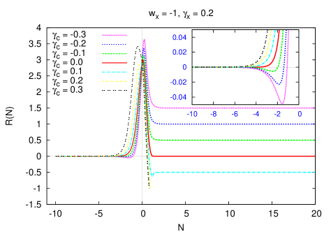
Figure 4: Examples of the DE-DM ratio $R$ as obtained from the numerical solutions of Eqs. (45), under the condition that all cases have $x_{0}=0.7$ and $y_{0}=0.24$ at $N=0$. We took a fixed value of $\gamma_{x}=0.2$ for the case $w_{x}=-1$, and the values of $\gamma_{c}$ are as indicated on the plot. Negative (positive) values of DE at early times appear for negative (positive) values of $\gamma_{c}$ (see the inset), and a finite late time attractor appears only if the condition $(\gamma_{x}-\gamma_{c})>0$ holds. The values for which $(\gamma_{x}-\gamma_{c})\leq 0$ lead to $x\to-\infty$, and may also break the constraint (60).

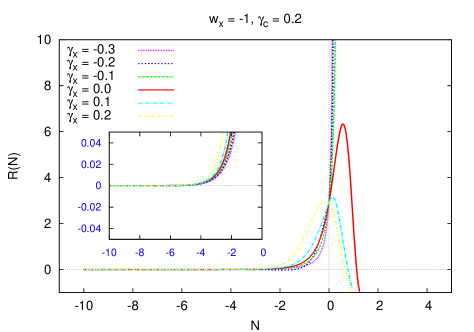
Figure 5: The same as in Fig. 4, but now for the fixed value $\gamma_{c}=0.2$. As expected, early evolution is positive because $\gamma_{c}>0$ (see the inset), but point C is unstable in all cases. The DE-DM ratio first diverges for $x_{0}<x^{+}_{*}$, but asymptotes to $R\to\pm-1$ at late times whatever the case $x_{0}>x^{+}_{*}$ or $x_{0}<x^{+}_{*}$, see Sec. IV.2 and Eqs. (49).

V Conclusions

We have made a careful analysis of two simple models of interaction between DM and DE. The first model, Model I, has an interaction term proportional to the Hubble parameter times a linear combination of the dark sector densities, and is one of the most studied in the literature.

We developed different mathematical techniques to investigate the properties of the model under simple but general enough assumptions. Our results recover those of previous studies, and we found new analytic expressions that clarify the limitations of Model I.

To begin with, we absorbed the (constant) DE equation of state $w_{x}$ into the equations of motion, so that the parameter-space is truly 2-dimensional; this very much simplified the study of the allowed values of the interaction parameters (compare our Fig. 1 with the corresponding 3-dimensional figures in Quartin et al. (2008)).

The absorption of the equation of state is not a mere mathematical trick. The original equations of motion would have been

$$x^{\prime} = -3w_{x}x\left(1-x\right)-z\,,$$ (61a)

$$y^{\prime} = 3w_{x}xy+z\,.$$ (61b)

We can see that Eqs. (8) are recovered by setting $w_{x}=-1$ in the above equations. Thus, the cases discussed are in some sense isomorphic to the cosmological constant interacting case.

This fact also shows the degeneracy between interacting models with a constant DE equation of state; if there is a successful model with a cosmological constant, one can find another one with a different value of $w_{x}$. However, the models are distinguishable in their particular evolution, as the DE equation of state should appear explicitly in the final expression of the DE-DM ratio, see Eq. (27), and other quantities.

Even though our general assumption was $w_{x}<0$, it is clear that in practice we have to restrict ourselves to values of the DE equation of state that allow an accelerating expansion at the present time, i.e. $w_{\rm tot}<-1/3$. It is also possible to allow phantom values $w_{x}<-1$, although it is not clear whether any physically consistent models exist in this regime. A comparison with observations would then be required to distinguish among the different possibilities, but this is beyond the purposes of the present study.

We presented for the first time the surprisingly simple equation (12) for the DE-DM ratio, and its simple analytic solution (27). We stress that the exact solution (27) allows us to easily and directly uncover the limitations of this interaction model. The exact solution has only one free integration constant, and thus we need a careful choice of initial conditions ensure an evolution that remains close to that of the standard non-interacting cosmology.

Surprisingly restrictive limitations are needed on the interaction parameters, $\alpha_{c}$ and $\alpha_{x}$. Our simplified study of the parameter space showed that the parameters should take very small values. This is also in agreement with other studies in which one can find a careful comparison of the model with cosmological observations (see for instance Quartin et al. (2008); del Campo et al. (2008, 2009); Olivares et al. (2008); Guo et al. (2007)). We showed that the model that seems to work better is the simple case $\alpha_{c}=0$. This model is almost indistinguishable from the standard $\Lambda$CDM at early times, but provides a finite DE-DM ratio at late times so that the coincidence problem is alleviated.

Other interesting properties arise from the interacting Model II of Sec. IV. Even though it can be thought of as a time-dependent version of Model I, the properties of the critical points differ significantly.

First of all, its vanishing interaction variables at early times allow Model II to have a true matter dominated epoch, which in fact corresponds to a (unstable) critical point of the dynamical system. However, a positive DM interaction $\Gamma_{c}>0$ is necessary in order to keep the DE component positive at early times.

Also, the DE-DM ratio can be finite and positive at late times, but this requires the dark interactions to have opposite signs and to comply with the condition $\Gamma_{x}>\Gamma_{c}$. It is then apparent that we cannot, in general, have a realization of Model II in which the dark components are well behaved for all times and the coincidence problem is addressed.

There is though a simple model that may be realistic and corresponds to $\Gamma_{c}=0$. This model can satisfy all the constraints and the DE interaction $\Gamma_{x}$ can be adjusted so that the Universe can have appropriate matter and DE eras. The only difference is that DE domination is a transient event: the Universe would eventually go back to a DM dominated epoch at late times.

Finally, we note that the problem of negative dark sector densities is not the only problem with Models I and II: the curvature perturbation also has a non-adiabatic instability on large scales Valiviita et al. (2008). As pointed out in Valiviita et al. (2008), both of these pathologies in the interaction models are related to the way in which we treat DE, i.e. as a fluid with constant $w_{x}$. If $w_{x}$ is allowed to vary in the early universe (as happens with scalar field DE), then the pathologies can be avoided.