Spectral Modeling of Rotating Turbulent Flows

Abstract

We test a subgrid-scale spectral model of rotating turbulent flows against direct numerical simulations. The particular case of Taylor-Green forcing at large scale is considered, a configuration that mimics the flow between two counter rotating disks as often used in the laboratory. We perform computations in the presence of moderate rotation down to Rossby numbers of 0.03, as can be encountered in the Earth atmosphere and oceans. We provide several classical measures of the degree of anisotropy of the small scales of the flows under study and conclude that an isotropic model may suffice at moderate Rossby numbers. The model, developed previously (Baerenzung et al., Phys. Rev. E 77, 046303 (2008)), incorporates eddy viscosity that depends dynamically on the inertial index of the energy spectrum, as well as eddy noise. We show that the model reproduces satisfactorily all large-scale properties of the direct numerical simulations up to Reynolds numbers of $\sim 10^{4}$ and for long times after the onset of the inverse cascade of energy at low Rossby number.

I Introduction

Rotating flows are commonplace in nature, the influence of rotation being measured by the Rossby number $Ro=U_{0}/2L_{0}\Omega$, with $U_{0}$ the r.m.s. velocity, $L_{0}$ a characteristic lengthscale of the flow and $\Omega$ the rotation rate. The Rossby number of the atmosphere is $\sim 0.1$ and in the ocean it can be as small as $10^{-3}$. Assuming a constant rotation rate, the Coriolis force that appears in the equations leads to the emergence of wave motions which, at small enough Rossby number, can be thought as dominating the dynamics. However, at high Reynolds number, $Re=U_{0}L_{0}/\nu$, with $\nu$ the viscosity, turbulent eddies interact with waves, and inertial waves interact nonlinearly (in particular through resonances), so that the dynamics become complex. The Rossby number can be viewed in this way as the ratio of the characteristic time of an inertial wave, $\tau_{W}\sim 1/\Omega$ to the characteristic time of an eddy, or eddy turn-over time, $\tau_{NL}\sim L_{0}/U_{0}$; when small, the waves are rapid and may dominate the dynamics.

Many studies have been devoted to the exploration of rotating turbulence, experimental as well as numerical and theoretical (see e.g.[1]). One expects the flow to become quasi bi-dimensional under the influence of strong rotation but recent studies show that the dynamics is more subtle, with three-dimensional eddies possibly prevailing at small scales. The case of small Rossby number can be studied using anisotropic extensions of closure models, such as the Eddy Damped Quasi Normal Markovian approximation (EDQNM hereafter). In such approaches, the closure is obtained by modeling the damping of fourth-order cumulants (non-zero for a non Gaussian field) by a term linear in third-order moments; dimensionally, the constant of proportionality is the inverse of a time, or a rate $\mu$, taken in EDQNM to be the rates known to be significant in the physics of the problem. In the simplest case of non-rotating isotropic and homogeneous turbulence, these rates are proportional to the inverse of the eddy turn over time $\tau_{\ell}=\ell/U_{\ell}$ and of the viscous time $\tau_{D}\sim\ell^{2}/\nu$, expressed in terms of the scale $\ell$ and the velocity at that scale $U_{\ell}$. In the rotating case, the wave frequency becomes relevant as well [2] (see [3] for an early realization of this concept), and because of the anisotropic dispersion relation of inertial waves, the model becomes anisotropic itself in terms of a spectral energy distribution that is a function of the wavenumbers $k_{\perp}$ and $k_{\parallel}$ , where $\perp$ and $\parallel$ refer to directions relative to the rotation axis.

Other approaches include weak turbulence theory [4], following the original methodology of Benney and Newell [5], and other resonant wave theories [6, 7] recently shown to correspond to an asymptotic limit for flows with wave dynamics [8].

The link between resonant theories and the EDQNM closure for rotating flows has been analyzed in detail recently ([9, 10] and references therein); it can be simply said here that when the global damping rate $\mu$ (omitting triadic scale dependence) is dominated by the inertial frequency, in the limit of $\tau_{W}\rightarrow 0$, the fourth-order cumulant becomes negligible, the flow becomes quasi-gaussian and the closure occurs naturally. Of course, this limit needs to be taken carefully, in particular when approaching the slow manifold ($k_{\parallel}=0$) [11, 9], possibly because of what could be called interferences between resonant modes and modes in the slow manifold.

The Coriolis force does not affect the kinetic energy balance nor does it modify the nonlinear part of the exact law stemming from energy conservation [12, 13] when stated in its anisotropic version. Similarly, helicity conservation is not altered by the Coriolis force, nor is (in the structure function formulation) the nonlinear part of the exact law stemming from that conservation [14]: indeed, helicity is conserved in the presence of rigid body rotation and, when using structure functions as in [14], the constant rotation vector drops from the dynamical equation for the second order moment. The fact that uniform rotation affects odd-order moments of the velocity but not even ones (at least in the linear limit of negligible nonlinear terms) shows that its effects are subtle. However, it has been documented in the literature (see e.g. [15]) that a specific model is needed in Large Eddy Simulations (LES) of turbulent rotating flows in order to take into account the slowing down of energy decay because of waves [16], and the anisotropy of integral length scales and of dissipation.

Furthermore, wave resonant theories are non uniform in scale and it is not clear whether their predictions are verified in high Reynolds number flows in the laboratory, in the environment or in direct numerical simulations (DNS). In the decaying case [17], there may be different temporal regimes in which different mechanisms prevail [10]. In a forced flow, high resolutions and long-time integrations are needed in order to resolve the different spatial regimes that may develop (e.g. inverse and direct cascades of energy [18, 19, 20, 21, 22] and direct cascades of helicity [23]), as well as the short-time wave regime versus the long-time turbulent regime.

Modeling becomes a necessity in order to reach an understanding of these flows at high Reynolds numbers as occurs in astrophysics and geophysics. Using a closure set of integro-differential equations for the energy spectra (see [10] and references therein) or the weak turbulence framework developed in [4] is a powerful tool for sufficiently small Rossby number, but two difficulties have to be overcome. On the one hand, such techniques are valid in the limit $Ro\rightarrow 0$ and yet the flows one tries to model may present inhomogeneities (in space, in time, in scale) that are affected differently by the rotation. On the other hand, the complexity of the so-called weak turbulence kinetic equations and in particular their dependence on the angle between the wavevector (in a Fourier decomposition) and the rotation axis (to be taken as the z axis in what follows) necessitates a regular discretization in angle as opposed to an exponential discretization in wavenumber, the latter working because of the self-similarity of the known (power law) spectral solutions to the equations. This angular dependency makes the closure or weak turbulence equations difficult and costly to use (see however [10]).

The anisotropy of a rotating flow comes from the nonlinear terms (and resonant triadic interactions) [16], at least for one-time second order statistics [24], because of a loss of phase information. An explicit example of an initial condition that gives rise to elongated vortices is given in [16]; these authors predict linear growth of the integral scale, as opposed to the classical Kolmogorov $\sim t^{2/7}$ law, and as observed in laboratory experiments [17]. This anisotropy is also linked to an asymmetry (predominance of cyclonic event over anti-cyclonic) for times of order $1/\Omega$, as measured for example by the skewness of the vertical component of the vorticity [25, 26]. However, it has been shown by several authors that the expected bi-dimensionalization of the flow is only realized partially, and small scale eddies may not follow such a dynamics; in which case, one expects the small scale eddies (i.e., those that are to be modeled in an LES approach) to be somewhat isotropic. It may thus be envisageable to use, as a model of small scales, a methodology developed for isotropic flows.

It is in this context that we extend the spectral model derived in [27] to the case of forced rotating flows, comparing the results of the model to high resolution DNS [22] for forced rotating turbulence down to $Ro\sim 0.03$. The model is based on the EDQNM closure to compute eddy viscosity and eddy noise. It adapts dynamically to the inertial index of the energy spectrum, and as a result it is well suited to study rotating turbulence for which the scaling laws are not well known, and may change with the Rossby number, and also (at fixed Rossby number) as the system evolves and an inverse cascade develops. The next section poses the problem in terms of equations and models and gives the numerical set-up. We then describe the results for the isotropic LES model, examining energetic balance, structures, spectra and higher-order statistics. Finally, the last section presents our conclusions.

II Equations and spectral modeling

II.1 Primitive equations

The dynamical equations can be written in terms of the Fourier coefficients of the velocity field defined as usual as:

$$\textbf{v}(\textbf{k},t)=\int\!\!\!\int\!\!\!\int_{-\infty}^{\infty}\textbf{v}(\textbf{x},t)e^{-i\textbf{k}.\textbf{x}}\textbf{dx}\ .$$ (1)

In the rotating frame, and including the centrifugal force in the pressure term, the equations are:

$$\left(\frac{\partial}{\partial t}+\nu k^{2}\right)v_{\alpha}(\textbf{k},t)+2\Omega P_{\alpha\beta}\varepsilon_{\beta z\gamma}u_{\gamma}(\textbf{k},t)={t_{\alpha}}(\textbf{k},t)+{F_{\alpha}}({\bf k})$$ (2)

together with the incompressibility condition ${\textbf{k}\cdot\textbf{v}}={\bf 0}$; $\nu$ is the kinematic viscosity, ${\bf F}({\bf k})$ is the Fourier transform of the forcing function, $P_{\alpha\beta}=\delta_{\alpha\beta}-k_{\alpha}k_{\beta}/k^{2}$ is the projection operator, $\Omega$ is the rotation rate and $\textbf{t}(\textbf{k},t)$ is a bilinear operator for the kinetic energy transfer written as:

$$t_{\alpha}(\textbf{k},t)=-iP_{\alpha\beta}(\textbf{k})k_{\gamma}\sum_{\textbf{p}+\textbf{q}=\textbf{k}}v_{\beta}(\textbf{p},t)v_{\gamma}(\textbf{q},t)\ .$$ (3)

Note that $P_{\alpha\beta}$ is a projector that allows us to take the pressure term of the velocity equation into account via a Poisson formulation and ensures that the velocity remains divergence-free including in the presence of rotation. Finally note that the total energy $E_{T}=\left<{\bf v}^{2}/2\right>$ and the helicity $\left<{\bf v}\cdot{\bf\omega}\right>$ (with ${\bf\omega}=\nabla\times{\bf v}$) are invariants of the three-dimensional equations in the ideal case, i.e. in the absence of viscous dissipation ($\nu=0$). Besides the Reynolds number and the Rossby number defined previously, one can also introduce dimensionless numbers based on small-scales as produced by the turbulent flow; the simplest way to do that, traditionally, is to base such parameters on the vorticity through the Taylor scale $\lambda$ defined as:

$$\lambda=2\pi\left(\frac{\int{E(k)dk}}{\int{E(k)k^{2}dk}}\right)^{1/2};$$ (4)

the Taylor Reynolds number is then:

$$R_{\lambda}=\frac{U_{0}\lambda}{\nu}\ .$$

One can also define a quantity called the micro-Rossby number [21] which is useful to determine the regime of the small scale turbulence and the slope of the energy spectrum [25]. It reads:

$$Ro_{\omega}=\frac{\omega_{rms}}{2\Omega},$$ (5)

where $\omega_{rms}$ stands for the $r.m.s.$ vorticity; note that it is proportional to the Rossby number evaluated at the Taylor scale. Finally, we also define the Ekman number:

$$Ek=\frac{Ro}{Re}=\frac{\nu}{2\Omega L_{0}^{2}},$$ (6)

where $L_{0}=2\pi/k_{0}$ is the scale associated with the forcing at $k_{0}=2$. The direct numerical simulations used in this paper (runs Id, IId and IIId respectively, see Table 1) in order to assess the validity of the LES are those labeled A3, A4 and A6 respectively in [22] (hereafter, paper I). For all these runs, the forcing function is a Taylor-Green (TG) vortex with amplitude $F_{0}$:

$${F_{x}} = F_{0}\sin(k_{0}x)\cos(k_{0}y)\cos(k_{0}z)$$

$${F_{y}} = -F_{0}\cos(k_{0}x)\sin(k_{0}y)\cos(k_{0}z)$$

$${F_{z}} = 0\ ;$$ (7)

the third component of the forcing is equal to zero but the velocity in the z-direction grows through nonlinear interactions. Moreover, the forcing injects no energy in modes with $k_{z}=0$, and as a result any amplification observed in strongly rotating cases must be only due to a cascade process. Finally, the resulting flow has a small spectral anisotropy with slightly more energy in the $z$ direction [22], an effect which is the opposite of the tendency towards two-dimensionalization that develops in rotating turbulence.

The numerical computations using the above forcing are thus either Direct Numerical Simulations of the Navier-Stokes equations with $256^{3}$ grid points, or Large Eddy Simulations on grids of $64^{3}$ points; the axis of rotation is the $z$-axis, and the flow is initially at rest. Note that the TG flow is widely used in experimental devices to study turbulence and its effect on the generation of magnetic fields [28] even though the TG vortex has no net helicity due to its symmetries; because of this latter property, the LES model used here will not include the helicity eddy viscosity derived in [27] (Paper II hereafter). The turnover time at the forcing scale is then defined as $\tau_{NL}=L_{0}/U_{0}$ where $U_{0}=\sqrt{\left<{\bf v}^{2}\right>}$ is the r.m.s. velocity measured in the turbulent steady state as stated previously, at the onset of the inverse cascade at low Rossby number. Note that the amplitude of the forcing $F_{0}$ in each simulation is increased with $\Omega$ to have $U_{0}\approx 1$ in all the runs before the inverse cascade sets in (see [22] for more details on the DNS runs).

Finally, as the issue of the direction of the energy cascade (direct and/or inverse) is an important issue in rotating turbulence, a useful diagnostic in this context is to examine the behavior of the skewness (normalized third-order moment corresponding to energy transfer) based on the velocity derivative,

$$S_{k}={\frac{\left<(\partial_{x}v_{x})^{3}\right>}{\left<(\partial_{x}v_{x})^{2}\right>^{3/2}}}\ .$$ (8)

II.2 The isotropic EDQNM closure

The Large Eddy Simulation model (LES) derived in [27] for non-rotating Navier-Stokes flows is now extended to the rotating case in its non-helical version (LES-P of Paper II). In other words, intrinsic variations of the helicity spectra are not taken into account in the present work in the evaluation of the transport coefficients used in our LES model. The first step of the model is to employ a spectral filtering of the equations; this operation consists in truncating all velocity components at wave vectors k such that $|\textbf{k}|=k>k_{c}$, where $k_{c}$ is a so-called cutoff wave number. Since the scales associated with $k_{c}$ are presumably much larger than the actual dissipative small scales in a high Reynolds number flow, one needs to model the transfer between the large (resolved) scales and the small (subgrid unresolved) scales of the flow. In order to approximate these transfer terms, the behavior of the energy spectrum after the cutoff wave number has to be estimated. We therefore define an intermediate range, lying between $k_{c}$ and $3k_{c}$, where the energy spectrum is assumed to present a power-law behavior possibly followed by an exponential decrease:

$$E^{V}(k,t)=E_{0}^{V}k^{-\alpha_{E}^{V}}e^{-\delta_{E}^{V}k},\quad k_{c}\leq k<3k_{c}\ .$$ (9)

The coefficients $\alpha_{E}^{V}$, $\delta_{E}^{V}$ and $E_{0}^{V}$ are computed at each time step, through a mean square fit of the resolved energy spectrum. In a second step, one can write the following model equations (omitting forcing):

$$\left[\partial_{t}+\left(\nu\left(k|k_{c},t\right)+\nu\right)k^{2}\right]v_{\alpha}(\textbf{k},t)$$

$$=t_{\alpha}^{<}(\textbf{k},t)-2\Omega P_{\alpha\beta}\epsilon_{\beta z\gamma}u_{\gamma}(\textbf{k},t) \ ,$$ (10)

where the $<$ symbol indicates that the nonlinear transfer terms are integrated over a truncated domain defined such that $\textbf{p}+\textbf{q}=\textbf{k}$ with $|\textbf{p}|=p,|\textbf{q}|=q<k_{c}$. The eddy viscosity $\nu\left(k|k_{c},t\right)$ is expressed as

$$\nu(k|k_{c},t)\!\!\!\ =\!\!\!\ -\iint_{\Delta^{>}}\!\!\!\theta_{{}_{kpq}}\frac{S_{E_{2}}(k,p,q,t)}{2k^{2}E^{V}(k,t)}\ dpdq\ .$$

The function $S_{E_{2}}(k,p,q,t)$ corresponds to the so-called absorption term (linear in the energy spectrum $E^{V}(k,t)$) in the EDQNM nonlinear transfer, lending itself in particular to an expression for the turbulent eddy viscosity, as is well known; $\Delta^{>}$ is the integration domain over (${\bf k}$, ${\bf p}$, ${\bf q}$) triangles, such that $p$ and/or $q$ are larger than $k_{c}$, and both $p$ and $q$ are smaller than $3k_{c}$.

Finally, to take into account the effect of the emission (eddy-noise) term involved in the EDQNM nonlinear transfer ($S_{E_{1}}(k,p,q,t)$), we use a reconstruction field procedure which enables us to partly rebuild the phase relationships between the three spectral components of the velocity field, as explained in detail in Paper II [27]. The functions $S_{E_{1}}(k,p,q,t)$ and $S_{E_{2}}(k,p,q,t)$ appearing in the transport coefficients used in the LES are written for completion in the Appendix. Note that, although isotropic, the subgrid model we use in this paper has an important feature: it adjusts dynamically to the energy spectrum instead of assuming a given spectral law, usually the classical Kolmogorov law, $E(k)\sim k^{-5/3}$. This allows for exploration of flows for which a theory to predict spectral indices is not available. Also note that the reconstruction procedure differs as well from traditional implementations insofar as it tries to keep the phase information of the small-scales.

III Rotation and isotropy

One of the effects of rotation on a flow is to induce anisotropy, as in the formation of large-scale columnar vortices. In that light, we explore in this section the anisotropic properties of a DNS at low Rossby number to see whether or not it is relevant to use a model based on isotropic assumptions to simulate a flow subjected to rotation. The LES model we propose to use approximates, as is customary, the transfer from the large to the small scales, but most of the modeled interactions are between small scales because of the value of $k_{c}$ (chosen to be in all cases larger than the energy injection wavenumber), and because most of the modes in a turbulent flow are in the small scales (recall that the number of modes in a given isotropic shell $k_{i}$ varies as $k_{i}^{2}$).

We therefore investigate now the properties of the small scales of flows forced with the Taylor-Green vortex (see Eq. 7) and subjected to rotation, with $k_{0}=2$ and at a Rossby number $Ro=0.03$; we perform a DNS on a grid of $256^{3}$ points and with the flow being initially at rest. To measure anisotropy, we introduce two different quantities, a spatial one and a spectral one, denoted respectively $I^{D}$ (for dimensional) and $I^{C}$ (for Craya [29]; see also [30]). Another measure of anisotropy linked to the so-called polarization anisotropy, following [31] (see also [32]), is discussed later in Section IV.2. The spatial coefficient $I^{D}$ evaluates the averaged ratio between the intensity of the velocity in the perpendicular direction $V_{\perp}(\textbf{x},t)$ and in the parallel direction $V_{\parallel}(\textbf{x},t)$, with $\perp,\ \parallel$ referring to the $z$-axis of rotation. The velocity field can be expressed as a function of these two components as ${\textbf{v}}(\textbf{x},t)=V_{\parallel}(\textbf{x},t){\textbf{e}_{\parallel}}+{\bf V_{\perp}}(\textbf{x},t)$, where ${\textbf{e}_{\parallel}}$ is the unit vector associated to the axis of rotation and ${\textbf{V}}_{\perp}(\textbf{x},t)$ is the velocity field projected on the plane perpendicular to ${\textbf{e}_{\parallel}}$.

The spatial anisotropy coefficient therefore reads:

$$I^{D}=\left<\frac{V_{\perp}(\textbf{x},t)}{V_{\parallel}(\textbf{x},t)}\right>\ .$$ (11)

The spectral coefficient $I^{C}$ is computed as in [34]: for each wavevector ${\bf k}$, an orthonormal reference frame is defined as (${\bf k}/|{\bf k}|$, ${\bf e}_{1}({\bf k})/|{\bf e}_{1}({\bf k})|$, ${\bf e}_{2}({\bf k})/|{\bf e}_{2}({\bf k})|$), with ${\bf e}_{1}({\bf k})={\bf k}\times{\bf z}$ and ${\bf e}_{2}({\bf k})={\bf k}\times{\bf e}_{1}({\bf k})$, where ${\bf z}$ is the vertical unit wavevector. In that frame, since the incompressibility condition yields ${\bf k}\cdot{\bf v}({\bf k})=0$, ${\bf v}({\bf k})$ is only determined by its two components ${\bf v}_{1}({\bf k})$ and ${\bf v}_{2}({\bf k})$. This second anisotropy coefficient is then defined as

$$I^{C}=\sqrt{\left<|{\bf v}_{1}({\bf k})|^{2}\right>/\left<|{\bf v}_{2}({\bf k})|^{2}\right>}\ .$$ (12)

Both $I^{D}$ and $I^{C}$ are such that they have unit values for fully isotropic flows.

In Fig. 1 we plot the temporal evolution of the total energy, the time being expressed in units of the eddy turn-over time. Note the long interval before turbulence fully develops, as rotation is strong and the run was started from a fluid at rest. Indeed, before the energy starts to grow at $t\approx 90$, one can observe a long transient during which the energy displays damped oscillations in time (see Paper I). This transient is linked to the effect of rotation and its duration increases linearly with $\Omega$, i.e. as the inverse of the Rossby number. During this first stage, the energy dissipation rate is small and the energy spectrum is very steep. Later, at $t\approx 90$, the enstrophy starts to grow and the energy dissipation rate increases. The energy also grows and an inverse cascade of energy develops. Turbulence sets in and the small-scale energy spectrum develops an inertial range with scaling close to $\sim k_{\perp}^{-2}$ (see Paper I for more details).

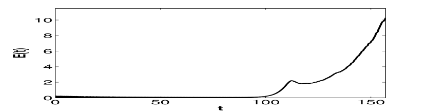
Figure 1: Temporal evolution of the energy for the flow in a DNS with $Ro=0.03$; it displays two temporal phases, one dominated by wave interactions and one, for t larger than $100$, corresponding to an inverse cascade of energy.

In order to quantify the importance of anisotropy at what would be the sub-grid scales in a LES of rotating flows, we start by noting that the velocity (in particular when an inverse cascade of energy develops at small enough Rossby number) is dominated by the large scales whereas the modeling will occur in the small scales of the flow. In this context, we introduce a band-pass filter of the DNS data in order to concentrate the analysis on small-scale properties of the flow. The filtered field is given in Fourier space by all the velocity components at a wavector k such that $32\leq|\textbf{k}|\leq 64$; note that, for this DNS using a classical 2/3 dealiasing rule, the maximum wavenumber is $k_{max}=85$. As a result, the band-pass filter can be interpreted as preserving the small scales of the direct cascade inertial range.

Figure 2 represents the time history of the $I^{C}$ and $I^{D}$ anisotropy coefficients for the complete DNS (dash line) and for the band-pass filtered velocity fields of the flow at $Ro=0.03$ (ovals). The Craya spectral coefficient $I^{C}$ of the complete DNS field remains close to unity during the whole simulation, indicating that globally the flow is close to an isotropic state. However, the directional coefficient $I^{D}$ exhibits three different regimes in the full DNS: a first phase between $t=0$ and $t\simeq 40$ during which it oscillates, with an amplitude that decreases with time, and a second phase, between $t\simeq 40$ and $t\simeq 90$, with this coefficient remaining constant at a value close to unity, meaning that no direction is privileged in the flow. Finally, in a third and last phase, which begins when the turbulence starts to develop, $I^{D}$ strongly increases with time. This behavior is the signature of the generation of intense columnar structures within the flow, within which the perpendicular component of the velocity field dominates the parallel one.

The behavior of these coefficients is completely different for the filtered, small-scale, field. Indeed, the small scales are strongly anisotropic during the transient period before the turbulence develops, with a maximum value for $I^{C}$ of the order of $3$ (and $5$ for $I^{D}$). In this phase, the directional anisotropy coefficient clearly shows that the perpendicular component of the velocity dominates the parallel one, and therefore that the small scales are mostly bi-dimensional. At $t\simeq 80$, both coefficients drop rather abruptly to a value of order unity, indicating that when the turbulence develops the small scales become isotropic corresponding to a standard cascade of energy to small scales (note that the scales for which the anisotropic and inverse accumulation of energy takes place are eliminated by the band-pass filter).

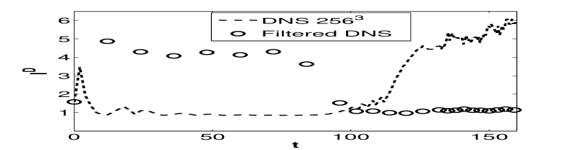
Figure 2: Temporal evolution for a flow with $Ro=0.03$ of the Craya anisotropy coefficient $I^{C}$ (top) and the directional anisotropy coefficient $I^{D}$ (bottom) (see eqs. 11, 12), for the full DNS velocity field (dash line) and the filtered DNS field (ovals) defined as a band-pass filter for wavevectors in $|K|\in[32,64]$. Note the sharp transition towards isotropy of the small scales for $t\simeq 100$, as both the direct and inverse turbulence cascades finally develop.

With this study of the small-scale behavior of a flow subjected to moderate rotation, we see that an isotropic LES model cannot be used to treat every phase of the flow. Indeed, in the early transient phase, a model based on isotropic assumptions will not be able to approximate properly the transfer between the subgrid scales and the resolved scales. We therefore decide to only use our model to study the turbulent regime of rotating flows, after $t\approx 100$ in the case of Figs. 1, 2. Moreover, this is consistent with the fact that a LES is designed to study turbulent flows, and cannot handle transitional (laminar, wave-dominated) flows. In the case of rotating flows starting from a fluid at rest, turbulence only develops after a transient time that depends linearly with the magnitude of the rotation. Note that in many studies, simulations of rotating flows are started from a previous turbulent steady state, and in that case our LES should have no problem to adapt as the spectral index changes with the evolution of the system.

Note that both coefficients $I^{C}$ and $I^{D}$ are relevant quantities in the context of this EDQNM-based LES: the behavior of $I^{C}$ justifies the assumption of “spectral isotropy” (i.e., dealing with $k$ instead of $(k_{||},k_{\perp})$ at small scales); on the other hand, the behavior of $I^{D}$ justifies the isotropic reconstruction done with the eddy-noise, because $I^{D}\approx 1$ is a measure of variance isotropy.

IV Numerical tests of the LES

We now test our LES model against direct numerical simulations with different Rossby numbers. As stated before, the forcing used is the Taylor-Green vortex (see Eq. 7) at $k_{0}=2$. For each simulation, we follow the numerical procedure described in Paper I; namely, we vary the rotation rate leading to three different Rossby numbers: $0.03$, $0.17$, and $0.35$. The simulation parameters are summarized in Table 1. The flow evolves in a periodic box, with $256^{3}$ grid points for the DNS and $64^{3}$ grid points for the LES. The “reduced-DNS” results, in the table and figures, refer to the filtered DNS data on a grid of $64^{3}$ grid-points, corresponding to the limited information contained in the LES grid. Since we are interested in studying only the modeling of the turbulent regime, we start the LES simulations from the reduced-DNS data at a time after the end of the transient phase. However, if the LES is started from a fluid at rest (i.e., started like the DNS at $t=0$), no significant differences are observed with the procedure of starting the LES at the end of the transient phase, except that the transient regime in the flow with $Ro=0.03$ is shorter. This accelerated evolution of the LES at low Rossby number during the transient when compared to the DNS can be easily explained considering the inclusion of transport coefficients in the LES which assumes that a turbulent flow is already present.

Table 1: Parameters of the simulations: Resolution $N^{3}$, Rossby number $Ro$ based on the forcing scale $L_{0}$, Taylor microscale $\lambda$ and integral scale $L$, r.m.s.velocity $U_{0}=\left<{\bf v}^{2}\right>^{1/2}$, integral Reynolds number $Re=$$\ U_{0}L/\nu$ and eddy turnover time $\tau_{NL}=L_{0}/U_{0}$; $t_{m}$ is the final time of the computation. Note that the r label in the nomenclature of the runs stands for reduced data obtained by filtering in spectral space to $64^{3}$ points the original $256^{3}$ DNS data $\lambda$, $L$, $Re$ and $\tau_{NL}$ are evaluated at the final time of the simulation for runs I which undergoes an inverse cascade, whereas they are averaged during the stationary phase of simulations II and III which are at higher Rossby numbers and do not undergo any significant inverse energy transfer.

		$N$	$Ro$	${\lambda}$	$L$	$U_{0}$	$Re$	$\tau_{NL}$	$t_{m}$
Id	DNS	$256$	$0.03$	$2.06$	$5.71$	$4.53$	$12920$	$1.26$	$157$
Ir	Reduced-DNS	$64$	–	$2.37$	$5.71$	$4.53$	$12927$	$1.26$	–
IL	LES	$64$	–	$2.07$	$5.59$	$4.60$	$12857$	$1.22$	–
IId	DNS	$256$	$0.17$	$0.65$	$1.44$	$1.01$	$729$	$1.41$	$45$
IIr	Reduced-DNS	$64$	–	$0.73$	$1.45$	$1.01$	$732$	$1.44$	–
IIL	LES	$64$	–	$0.76$	$1.49$	$1.09$	$813$	$1.36$	–
IIId	DNS	$256$	$0.35$	$0.77$	$1.47$	$1.07$	$786$	$1.36$	$45$
IIIr	Reduced-DNS	$64$	–	$0.72$	$1.41$	$0.96$	$678$	$1.46$	–
IIIL	LES	$64$	–	$0.75$	$1.42$	$0.98$	$695$	$1.45$	–

IV.1 Global behavior of the flow

The first test of the model is to examine the temporal evolution of the flow. This is displayed in Fig. 3 for the three Rossby numbers analyzed. The overall behaviors of the DNS and of the LES are similar in amplitude and in time scales. At intermediate Rossby numbers ($Ro=0.17$), the precise evolution of the DNS is not followed although the energy obtained with the LES remains close to the DNS one. For the simulation at $Ro=0.03$, an inverse cascade develops after $t\sim 120$ leading to a strong increase of the total energy. Although the LES model does not take wave interactions explicitly into account, it allows to reproduce this transfer of energy from the small scales to the very large ones with good accuracy; indeed, a scaling argument shows that in the small scales, the eddy turn-over time is shorter than the time associated with waves and nonlinearities prevail. The LES is taking into account the interactions with the waves in an implicit way by changing the EDQNM time scale dynamically with the slope of the energy spectrum at large scales; this could be interpreted as “reversed” Kraichnan-like phenomenology. Note that the run at intermediate Rossby number has higher values of the energy because the forcing amplitude is larger than for the run at $Ro=0.35$.

When looking at the time-averaged isotropic energy spectra (see Fig. 4) for the two flows at the largest Rossby numbers, one can see that a good agreement is obtained. This figure also allows us to better understand the difference in the temporal evolution of the energy computed from the DNS and the LES data at $Ro=0.17$ (see Fig. 3). Indeed, although the model gives a good estimation of the DNS spectra at small scales, at very large scale (and particularly at $k=2$) non-negligible differences appear with the DNS, differences to which the total energy is sensitive. Note that a smaller difference between LES and DNS spectra can be observed at $k=2$ for the run at the higher Rossby number, $Ro=0.35$. Otherwise, the spectrum is well approximated by the LES at all the other scales.

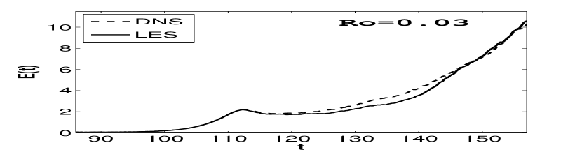
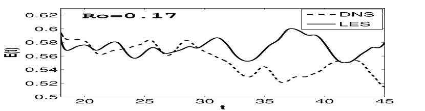
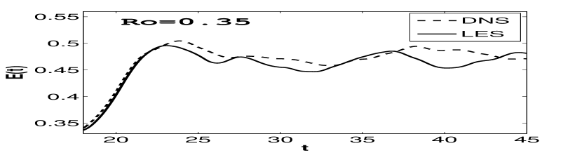
Figure 3: Temporal evolution of the total energy for runs Id (DNS: $256^{3}$) and IL (LES: $64^{3}$) at $Ro=0.03$ (top), runs IId (DNS: $256^{3}$) and IIL (LES: $64^{3}$) at $Ro=0.17$ (middle),and runs IIId (DNS: $256^{3}$) and IIIL (LES: $64^{3}$) at $Ro=0.35$ (bottom). DNS runs with dash line, LES runs with solid line. Note the change of values on both axes for the low Rossby runs (top) because of the delay in the development of the turbulent phase, when the LES is started, and the ensuing accumulation of energy due to the inverse cascade now taking place at that low Rossby number.

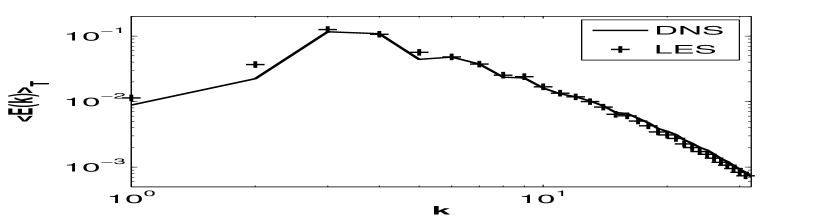
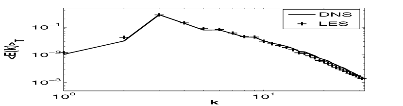
Figure 4: Time averaged energy spectra for runs IId (DNS: $256^{3}$) and IIL (LES: $64^{3}$) at $Ro=0.17$ (top), and runs IIId (DNS: $256^{3}$) and IIIL (LES: $64^{3}$) at $Ro=0.35$ (bottom). Time averaging is performed from $t=25$ to $t=45$ for both simulations. Note the good agreement except possibly near $k=2$ corresponding to the forcing scale, indicative of a lack of adjustment of the LES at that scale, in particular for the perpendicular spectra, see Fig. 5.

Similarly, when decomposing the energy spectra into their perpendicular and parallel components, a good agreement is reached at large scales, except again at $k=2$ for the perpendicular spectrum of the flow at $Ro=0.17$ (see Fig. 5). On the contrary, at small scales, the model seems to underestimate the spectra obtained by the DNS. This behavior is in fact due to the difference in resolution between the DNS and the LES: as $k_{\perp}$ and $k_{\parallel}$ increase, the difference between the amount of modes taken into account in the evolution of these spectra for the DNS and for the LES increases as well. Note that the $k_{||}$ shells have the same number of modes independently of the value of $k_{||}$ (they are planes), while the number of modes in the $k_{\perp}$ shells grow as $k_{\perp}$ (they are cylinders), and this number grows as $k^{D-1}$ in dimension $D$ for isotropic (spherical) shells. We have checked that,when making the comparison between the LES and the reduced DNS for instantaneous spectra, the discrepancy observed at high wavenumber disappears.

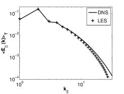
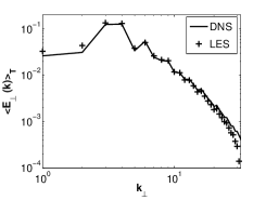
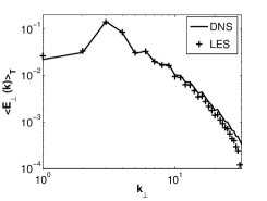
Figure 5: Time averaged parallel (left) and perpendicular (right) energy spectra, for runs IId (DNS: $256^{3}$) and IIL (LES: $64^{3}$) at $Ro=0.17$ (top), and runs IIId (DNS: $256^{3}$) and IIIL (LES: $64^{3}$) at $Ro=0.35$ (bottom).

As mentioned earlier, the micro-Rossby number measures how strong the imposed rotation is in the flow at the Taylor microscale, when compared to the r.m.s. vorticity developed by the turbulence. Its time evolution is shown in Fig. 6 for all runs. Because the micro-Rossby number emphasizes small scales that are not all present in an LES, $Ro_{\omega}$ is also computed in the reduced-DNS. We observe a good agreement between the truncated DNS and the LES, although the model slightly underestimates $Ro_{\omega}$ for the two simulations at larger Rossby number. This behavior can be explained by enstrophy production in the LES, and the backscattering of energy from sub-grid scales to resolved scale associated to the eddy noise, which is perhaps not strong enough.

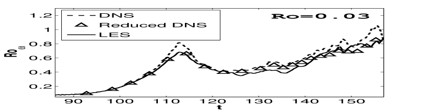
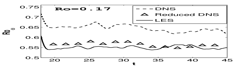
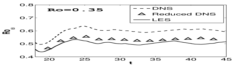
Figure 6: Temporal evolution of the micro Rossby number $Ro_{\omega}$ in flows with $Ro=0.03$ (top), $Ro=0.17$ (middle) and $Ro=0.35$ (bottom), for DNS on $256^{3}$ grid points (dash line), filtered data of the DNS to a $64^{3}$ grid (triangles) and LES (solid line) on a $64^{3}$ grid. Note again the different scale on the axes, in particular for the lowest Rossby number in which case $Ro_{\omega}$ approaches unity as the inverse cascade develops and energy and turbulence intensity grow.

In Table 2 we give the values of the characteristic parallel and perpendicular integral length scales (respectively $L_{\parallel}$ and $L_{\perp}$) defined as:

$$L_{\parallel} = \frac{\int_{1}^{k_{max}}E(k_{\parallel})k_{\parallel}^{-1}dk_{\parallel}}{\int_{1}^{k_{max}}E(k_{\parallel})dk_{\parallel}}\ ,$$ (13)

$$L_{\perp} = \frac{\int_{1}^{k_{max}}E(k_{\perp})k_{\perp}^{-1}dk_{\perp}}{\int_{1}^{k_{max}}E(k_{\perp})dk_{\perp}}\ ,$$ (14)

and computed at the final simulation time of each flow (note that the $k_{\parallel}=0$ mode is not included in the definition). Even if the values obtained by the LES data do not exactly correspond to the DNS values, they remain close; their difference can be explained by the same argument evoked before on the slight discrepancy between LES and DNS parallel and perpendicular energy spectra. Note that the perpendicular length scale is significantly larger for the lowest Rossby number, but the parallel length scales are comparable in all three runs. This is linked to the fact that the inverse cascade of energy which takes place at low Rossby number is dominated by quasi-two-dimensional modes; the parallel spectrum does not undergo an inverse cascade, although energy does pile up at $k_{\parallel}=0$ mainly through resonant coupling of waves.

Table 2: Characteristic integral length scales $L_{\perp}$ and $L_{\parallel}$ measured at different times $t_{m}$ for the three different Rossby numbers studied in this paper. Note that, at the lowest Rossby number ($Ro=0.03$, runs I), the perpendicular integral length scale is significantly larger than for more moderate rotation, because of the inverse cascade.

		$t_{m}$	$L_{\perp}$	$L_{\parallel}$
Id	DNS	$157$	$5.73$	$2.99$
IL	LES	$157$	$5.63$	$2.95$
IId	DNS	$45$	$1.71$	$2.95$
IIL	LES	$45$	$1.74$	$3.22$
IIId	DNS	$45$	$1.76$	$2.69$
IIIL	LES	$45$	$1.83$	$2.71$

IV.2 Measures of anisotropy

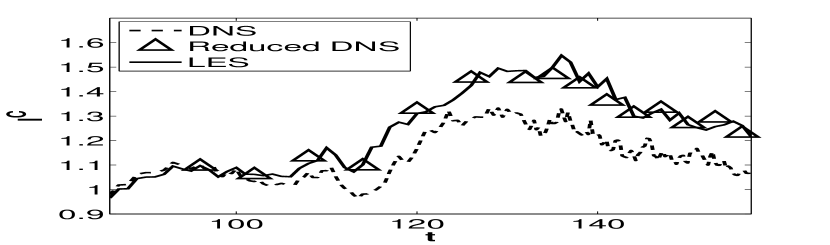
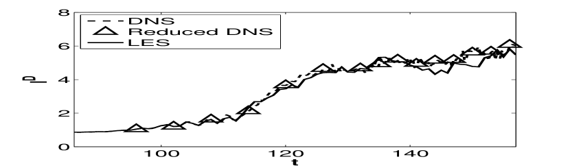
Figure 7: Evolution of the spectral and directional isotropy coefficients $I^{C}$ and $I^{D}$ (see text) for runs Ir (reduced DNS: $64^{3}$) and IL (LES: $64^{3}$) at low Rossby number ($Ro=0.03$). Information about the lower rotation cases is given in Table 3. Isotropy obtains when both coefficients are close to unity, and we note that the directional coefficient, related to real-space structures, indicates a stronger departure from isotropy than when measuring anisotropy in Fourier space as $I_{C}$ does (see Eqs. 11, 12), once the inverse cascade sets up and strong columnar vortices develop. Larger $I^{D}$ also obtain for the runs at lower Rossby numbers (see Table 3).

Rotating flows are known to develop anisotropies and we now turn our attention to this point. In order to estimate the anisotropy of the different flows, we use the coefficients $I^{D}$ and $I^{C}$ defined earlier in Eqs. (11) and (12). They are shown as a function of time in Fig. 7 for the DNS (dash line), the reduced DNS data truncated to the LES resolution (triangles), and the LES (solid line) with $Ro=0.03$. A very good match can be observed between the Craya coefficient $I^{C}$ computed from the reduced-DNS data and the one computed with the data from the LES model, whereas the coefficient computed with the full DNS data evolves on a lower level than the two other ones. This is due to the fact that the small scales of the field (i.e. scales with $k>k_{c}$) are taken into account in the spatial averaging process we perform to calculate this coefficient. We saw in Section III that these small scales are more isotropic with a corresponding coefficient $I^{C}$ near unity, so when they are taken into account in the computation of the Craya coefficient they lower its value. The small scales in the DNS are more isotropic, and as a result, the LES flow, which preserves a smaller amount of these scales, is globally more anisotropic and has a larger value of this coefficient.

As already observed in Fig. 2, the directional coefficient $I^{D}$ is strongly dominated by the large scales of the field, such as columnar structures appearing in the flow as a result of the inverse cascade process. Therefore, when we compare the time history of this coefficient for the DNS and the reduced-DNS, no noticeable difference appears. Once again our LES model predicts very well the evolution of this coefficient, even though the perpendicular component of the velocity clearly dominates over the parallel one. We also note that the model allows for a good estimation of both these coefficients for the simulations at larger Rossby numbers ($Ro=0.17$ and $Ro=0.35$), as shown in Table 3.

Table 3: Craya and directional isotropic coefficients $I^{C}$ and $I^{D}$ for the simulations at $Ro=0.17$ and $Ro=0.35$.

		$t$	$Ro$	$I^{C}$	$I^{D}$
IId	DNS	$45$	$0.17$	$1.05$	$1.69$
IIr	Reduced DNS	$45$	$0.17$	$1.07$	$1.69$
IIL	LES	$45$	$0.17$	$1.07$	$1.71$
IIId	DNS	$45$	$0.35$	$1.04$	$1.97$
IIIr	Reduced DNS	$45$	$0.35$	$1.04$	$1.97$
IIIL	LES	$45$	$0.35$	$1.04$	$2.01$

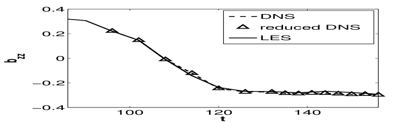
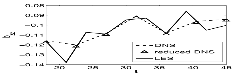
Figure 8: Temporal evolution of the $b_{zz}$ component of the polarization anisotropy tensor (see Eq. 15) for runs with $Ro=0.03$ (top) and $Ro=0.35$ (bottom), in the former case at late times once the pile-up of energy at large scales has begun. The DNS are plotted with a dash line, the reduced DNS, truncated to the resolution of the LES, are given with triangles and the solid line corresponds to the LES. Note again the tendency to a two-dimensional state at late times, with $b_{zz}\rightarrow-1/3$, for the low Rossby number runs.

In our investigation of anisotropy of rotating flows, we finally study the behavior of the $b_{ij}$ anisotropy tensor defined below (see e.g. [35] for reference); it is linked to the so-called “polarization” anisotropy introduced in [31] and as also discussed in [32] (see also [33]). This tensor, which is based on the Reynolds stress tensor $R_{ij}=\langle v_{i}(\textbf{x})v_{j}(\textbf{x})\rangle$, is defined as:

$$b_{ij}=\frac{R_{ij}}{R_{ll}}-\frac{\delta_{ij}}{3},$$ (15)

with summation upon the subscript $l$. In Fig. 8 we represent the temporal evolution of the $b_{zz}$ component of the anisotropy tensor for runs I and III, at respectively $Ro=0.03$ and $Ro=0.35$. We first notice that the LES model predicts well the evolution of this coefficient for both simulations. Secondly, the development of a preferred direction in the flow at $Ro=0.03$ (already observed in Fig. 7 through the increase of the directional coefficient $I^{D}$ in the inverse cascade), is also visible in this figure. Indeed, $b_{zz}$ tends to $-1/3$ as time increases, since $v_{z}(\textbf{x})$ becomes negligible when compared to the horizontal components $v_{x}(\textbf{x})$ and $v_{y}(\textbf{x})$.

IV.3 Statistical analysis

In this section, we investigate the statistics of the simulations at $Ro=0.03$. Instantaneous probability density functions (or PDFs) of the longitudinal and transverse derivative of the $x$-component of the velocity field are computed and plotted in Fig. 9 at time $t=132$, in the inverse cascade. The PDFs computed on the full DNS data, the reduced-DNS, and the LES, agree well for the case of the longitudinal derivative. In the case of the transverse derivative, the DNS data differ from both the LES and the reduced-DNS data, the latter two displaying wider wings and being almost superimposed. It is well known that the small scales of a flow may have a strong influence on the distribution of velocity derivatives with strong velocity gradients appearing at small scale, and that transverse derivatives show stronger tails in the pdfs (and therefore enhanced intermittency) than longitudinal derivatives. It is not clear whether this is the effect of more sensitivity to the intermittency in the transverse increments or whether it is the effect of small-scale anisotropy, but since the differences are stronger for the velocity derivatives taken in the direction of rotation, it may be attributed to anisotropies.

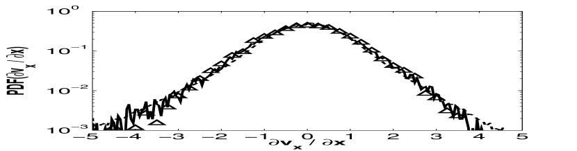
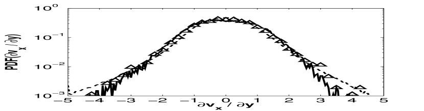
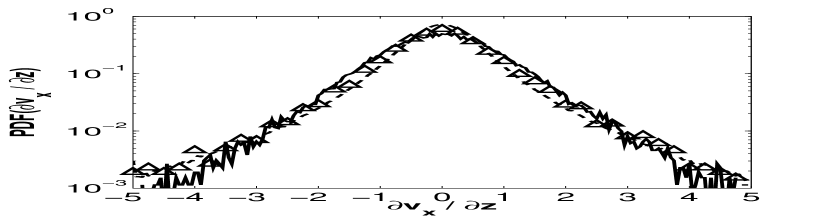
Figure 9: Probability density function of the velocity derivatives ${\partial v_{x}}/{\partial x}$ (top), ${\partial v_{x}}/{\partial y}$ (middle), and ${\partial v_{x}}/{\partial z}$ (bottom), for runs Id (DNS: $256^{3}$), Ir (reduced DNS: $64^{3}$), and IL (LES: $64^{3}$) at $Ro=0.03$ and $t=132$. As usual, dash line is for the full DNS flow, triangles for the reduced (truncated) DNS and solid line for the LES.

In order to quantify the distributions of velocity fluctuations and the differences between DNS and LES data, we now compute the skewness $S_{k}$ of the longitudinal velocity derivative, i.e. its normalized third order moment. The skewness, which measures the departure from Gaussian statistics, is usually negative for the longitudinal derivatives of a turbulent flow and oscillates around zero for the lateral ones. In Fig. 10 we show the time history of $S_{k}$. As for the energy, the LES model gives a correct prediction of the skewness for $86<t<145$, although around $t\simeq 140$, some discrepancy can be found that could be associated with the development of structures. Note that this difference can be also associated with a slight discrepancy in total energy at around the same time (see Fig. 3).

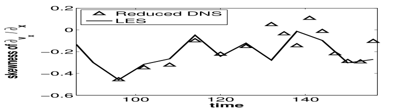
Figure 10: Temporal evolution of the skewness for the longitudinal velocity derivative ${\partial v_{x}}/{\partial x}$ (see Eq. 8), for runs Ir (reduced DNS: $64^{3}$) and IL (LES: $64^{3}$) at $Ro=0.03$.

IV.4 Visualization in physical space

We finally present a visualization in physical space of the velocity intensity at $t=132$ for the flow at $Ro=0.03$. At this time of the simulation the inverse cascade already took place and most of the flow energy was transferred to the $k_{\parallel}=0$ plane. We noted earlier that the TG flow injects no energy in the $k_{\perp}=1$ shell nor in the $k_{||}=0$ shell. So all energy we see at large scale is the result of inverse cascade (in the former case) and of two-dimensionalization (in the latter case). The evidence for the inverse cascade in this paper is given by the time evolution of the energy in Figs. 1 and 3 (see also Paper I, where fluxes are studied in detail). The accumulation of energy in this plane leads to the formation of columns as can be observed in Fig. 11. Although the structures are quasi-bidimensional, the isotropic LES model allows to reproduce them quite correctly. The spatial position differs slightly from the structure obtained by the DNS, but its size and intensity are well approximated. When examining the temporal evolution of the maximum of velocity (not shown), a good agreement occurs at all times. Note that this is a forced run visualized after $\approx 130$ turnover times; as a result of the intrinsic sensitivity of turbulent flows due to their inherent unpredictability after a Lyapounov time of the order of a few turn-over times, the spatial position of the structures is not expected to be reproduced exactly by the LES.

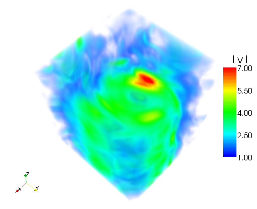
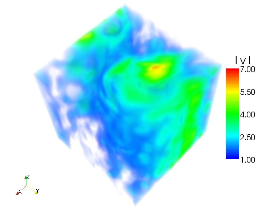
Figure 11: Volume rendering of the velocity modulus for flows at $Ro=0.03$ – runs Ir (Reduced DNS: $64^{3}$, top), and IL (LES: $64^{3}$ bottom) – at time $t=132$ for both simulations. The flow is dominated by a large eddy, but smaller vertical structures are visible as well.

V Conclusion

We present in this paper a Large Eddy Simulation model for high Reynolds number rotating flows using a previously derived sub-grid model [27] (see also [36]) based on the isotropic EDQNM two-point closure with eddy viscosity and eddy noise. We show that, down to Rossby numbers of $0.03$, the small-scales are sufficiently isotropic for the model to perform reasonably well. There are numerous laboratory experiments with which the comparison presented here could be extended, following the work in [21] using several EDQNM-based closures (see also [37] for the stratified anisotropic case). The advantage of using two-point closures such as EDQNM as a model for turbulent flows in the presence of rotation is that it allows for building scaling laws at a relatively low computational cost and with the possibility of doing analytical estimations of nonlinear transfer (see for example [21]). The model presented in this paper is much simpler since it is built on the isotropic three-dimensional version of the EDQNM; it is thus more limited in its scope insofar as it may not be able to explore very low Rossby numbers. On the other hand, following the standard LES methodology with spatially resolved large scales, and turbulent coefficients to model the sub-grid fluctuations, it allows to access more detailed features of the flows such as high-order statistics (e.g., PDFs) as well as spatial structures.

Also, the LES used in this paper adapts dynamically depending on the spectral index of the energy at super-filter (resolved) scales, and the value of the turbulent transport coefficients vary as a result. This is important in the context of rotating turbulent flows because the power law followed by the energy spectrum in this case is not quite ascertained yet and does vary with time. Phenomenological and theoretical predictions of this index, as well as several recent experiments, were reviewed in [25], with experimental and numerical evidence not quite able yet to sort out the different models or to fully describe the parameter space (e.g., as function of the rotation rate $\Omega$, the Reynolds number, etc.). An adequate LES model that can adjust to the resolved energy spectrum can help in this matter but more development and tests are needed. A reminiscent situation is found in magnetohydrodynamics (MHD) when coupling the fluid to a magnetic field in the non-relativistic limit; the total energy spectrum obtained analytically from the weak turbulence limit [38, 39] has been observed in the magnetosphere of Jupiter [40] and in DNS [41], but the strong turbulence spectrum (or spectra in case there are different regions in parameter space) is a matter of debate.

Only one specific (non-helical) forcing was explored in the DNS-LES comparisons studied in this paper. Further tests are required, considering other (non-helical) forcing functions, as well as forcing functions that introduce both energy and helicity in the flow. In this latter case, the implementation of the LES as described here may prove insufficient and one should also consider taking into account the spectral properties and turbulent transport coefficients that include the effect of helicity, as done in the non-rotating case in Paper II. Such an implementation can also be of interest for non-helical flows, because even though helicity is not a positive definite quantity, local helical fluctuations develop rapidly in a flow through alignment of vorticity and pressure gradients [42]. The properties of the model in the helical case in the presence of rotation will be dealt with in a forthcoming paper. The freely-decaying case (see [21, 10, 26] for a global perspective) needs to be examined as well and is left for future work.

As a final remark, we want to stress the importance of developing adequate modeling of rotating (and stratified) flows, as encountered for example in the Earth atmosphere. It was shown recently [43] that the maximum intensity of a hurricane depends crucially on the (assumed) horizontal mixing length; this implies that an adequate treatment of the turbulence is essential in predicting various properties of hurricanes such as its intensity or landfall localization. A run with resolution down to 62 meters shows strong local winds that were unresolved in previous studies [44]. If the work presented here (as well as most of its predecessors) is far from reality for hurricane dynamical modeling (because of its lack of proper boundary conditions, of stratification, of moisture, …), it nevertheless represents a first step towards the goal of a better understanding of geophysical flows, the issue here being that sufficiently high Reynolds number, i.e. sufficient multi-scale interactions and two-way coupling between the small scales and the large scales in turbulent fluids supporting inertial (and/or gravity) waves, is a desired ingredient for testing LES approaches to geophysical turbulence.

Appendix A Closure expressions of transfer terms

For completeness, we recall here the expression of the EDQNM closure equation for the kinetic energy spectrum $E(k,t)$ without helicity (note that the Coriolis term vanishes in the energy equation).

$$(\partial_{t}+2\nu k^{2})E(k,t)=\widehat{T}(k,t)$$ (16)

where the nonlinear transfer terms $\widehat{T}(k,t)$ is expressed as:

$$\widehat{T}(k,t)=\iint_{\Delta}\theta_{{}_{kpq}}(t)S_{E}(k,p,q,t)dpdq\ .$$ (17)

Here $\Delta$ is the integration domain with $p$ and $q$ such that (${\bf k},{\bf p},{\bf q}$) form a triangle, and $\theta_{{}_{kpq}}(t)$ is the relaxation time of the triple velocity correlations. As usual [45], $\theta_{{}_{kpq}}(t)$ is defined as :

$$\theta_{{}_{kpq}}(t)=\frac{1-e^{-(\mu_{k}+\mu_{q}+\mu_{p})t}}{\mu_{k}+\mu_{q}+\mu_{p}}\ ,$$ (18)

where $\mu_{k}$ expresses the rate at which the triple correlations evolve, i.e. under viscous dissipation and nonlinear shear. It can be written as:

$$\mu_{k}=\nu k^{2}+\lambda_{K}\Big{(}\int_{0}^{k}q^{2}E(q,t)dq\Big{)}^{1/2}\ .$$ (19)

Note that $\lambda_{K}$ is the only free parameter of the problem, taken equal to $0.36$ to recover the Kolmogorov constant $C_{K}=1.4$ for a $k^{-5/3}$ classical energy spectrum. The expressions of $S_{E}(k,p,q,t)$ can be further explicited (with the time dependency of energy spectra omitted here) as:

$$S_{E}(k,p,q,t) = \frac{k}{pq}b\left[k^{2}E(q)E(p)-p^{2}E(q)E(k)\right]$$

$$= S_{E_{1}}(k,p,q,t)+S_{E_{2}}(k,p,q,t)\ .$$

Here, $S_{E_{1}}(k,p,q,t)$, and $S_{E_{2}}(k,p,q,t)$, are respectively used to denote the two terms of the extensive expression of $S_{E}(k,p,q,t)$. The geometric coefficient $b(k,p,q)$ (in short, $b$ in the previous expression) is defined as:

$$b=\frac{p}{k}(xy+z^{3})\ ,$$ (20)

where here, $x$, $y$, $z$ are the cosines of the inner angles opposite to ${\bf k},{\bf p},{\bf q}$.

References

- [1] C. Cambon and P. Sagaut, Homogeneous Turbulence Dynamics. Cambridge Univ. Press, Cambridge (2008).
- [2] C. Cambon and L. Jacquin, “Spectral approach to non-isotropic turbulence subjected to rotation,” J. Fluid Mech. 202 , 295 (1989).
- [3] G. Holloway and M. Hendershott, “Stochastic closure for nonlinear Rossby waves,” J. Fluid Mech. 82, 747 (1977).
- [4] S. Galtier, “Weak inertial-wave turbulence theory,” Phys. Rev. E 68, 015301(R) (2003).
- [5] D. Benney and A. Newell, “Random Wave Closures,”Stud. Appl. Math. 49. 29 (1969).
- [6] H.P. Greenspan, The theory of rotating fluids. Cambridge Univ. Press, Cambridge (1968).
- [7] F. Waleffe, “Inertial transfers in the helical decomposition” Phys. Fluids A 5, 677 (1993).
- [8] P.F. Embid and A. Majda, “Averaging over fast gravity waves for geophysics flows with arbitrary potential vorticity” Commun. Partial Diff. Equat. 21, 619 (1996).
- [9] C. Cambon, R. Rubinstein and F.S. Godeferd, “Advances in wave turbulence: rapidly rotating flows,” New J. Phys. 6, 73 (2004).
- [10] F. Bellet et al., “Wave turbulence in rapidly rotating flows,” J. Fluid Mech. 562, 83 (2006).
- [11] L. Smith and F. Waleffe, “Transfer of energy to two-dimensional large scales in forced, rotating three-dimensional turbulence,” Phys. Fluids 11, 1608 (1999).
- [12] H. Politano and A. Pouquet, “Dynamical length scales for turbulent magnetized flows,” Geophys. Res. Lett. 25, 273 (1998).
- [13] E. Lindborg, “Kinematics of homogeneous axisymmetric turbulence” J. Fluid Mech. 302, 179 (1995).
- [14] T. Gomez, H. Politano & A. Pouquet, “An exact relationship for third–order structure functions in helical flows,” Phys. Rev. E, 61, 5321 (2000).
- [15] J. Bardina, J. Ferziger and R. Rogallo, “Effect of rotation on isotropic turbulence - Computation and modelling,” J. Fluid Mech. 154, 321 (1985).
- [16] P. Davidson, P. Staplehurst and B. Dalziel, “On the evolution of eddies in a rapidly rotating system,” J. Fluid Mech. 557, 135 (2006).
- [17] L. Jacquin et al., “Homogeneous turbulence in the presence of rotation,” J. Fluid Mech. 220, 1 (1990).
- [18] J. Bardina, J.H. Ferziger and R.S. Rogallo, “Effect of rotation on isotropic turbulence: computation and modeling” J. Fluid Mech. 154, 321 (1985).
- [19] P. Bartello, O. Métais and M. Lesieur, “Coherent structures in rotating three-dimensional turbulence” J. Fluid Mech. 273, 1 (1994).
- [20] L.M. Smith, J.R. Chasnov and F. Waleffe, Crossover from two- to three-dimensional turbulence. Phys. Rev. Lett. 77, 2467 (1996).
- [21] C. Cambon, N. Mansour and F. Godeferd, “Energy transfer in rotating turbulence,” J. Fluid Mech. 337, 303 (1997).
- [22] P.D. Mininni, A. Alexakis and A. Pouquet, “Scale interactions and scaling laws in rotating flows at moderate Rossby numbers and large Reynolds numbers,” in press Phys. Fluids (2008), see also http://arxiv.org/abs/0802.3714.
- [23] P.D. Mininni and A. Pouquet, “Helicity cascades in rotating turbulence,” submitted to Phys. Rev. E, see also arXiv:0809.0869 (2008).
- [24] J. Gence and C. Frick, “Naissance des corrélations triples de vorticité dans une turbulence statistiquement homogène soumise à une rotation,” C.R.A.S. Paris II 329, 351 (2001).
- [25] C. Morize, F. Moisy and M. Rabaud, “Decaying grid-generated turbulence in a rotating tank,” Phys. Fluids 17, 095105 (2005).
- [26] J. Seiwert, C. Morize and F. Moisy, “On the decrease of intermitency in decaying rotating turbulence,”Phys. Fluids 20, 071702 (2008).
- [27] J. Baerenzung et al., “Spectral modeling of turbulent flows and the role of helicity,” Phys. Rev. E 77, 046303 (2008).
- [28] M. Bourgoin et al., “An experimental Bullard von Kármán dynamo,” New Journal of Physics 8, 329 (2006).
- [29] A. Craya, “Contribution à l’analyse de la turbulence associée à des vitesses moyennes,” Thèse dans Publication Scientifiques et Techniques (1958).
- [30] J. Herring, Phys. Fluids 17, 859 (1974).
- [31] C. Cambon and L. Jacquin, “Energy transfer in rotating turbulence,” J. Fluid Mech. 202, 295 (1989).
- [32] Y. Morinishi, K. Nakabayashi and S.Q. Ren, “Dynamics of anisotropy on decaying homogeneous turbulence subjected to system rotation,” Phys. Fluids 13, 2912 (2001).
- [33] X. Yang and J.A Domaradzki, “Large Eddy Simulations of decaying rotating turbulence,” Phys. FLuids 16, 4088 (2004).
- [34] J.H. Curry et al., “Order and Disorder in Two and Three Dimensional Bénard Convection,” J. Fluid Mech. 147 , 1 (1984).
- [35] P. Sagaut and C. Cambon, “Homogeneous Turbulence Dynamics,” Cambridge University Press (2008).
- [36] J. Baerenzung, PhD Thesis, “Modélisation de la turbulence hydrodynamique et magnétohydodynamique,” Université de Nice-Sophia Antipolis, Observatoire de la Côte d’Azur (2008).
- [37] F. Godeferd and C. Staquet, “Statistical modelling and direct numerical simulations of decaying stably stratified turbulence. Part 2. Large-scale and small-scale anisotropy,” J. Fluid Mech. 486, 115 (2003).
- [38] S. Galtier et al., “A weak turbulence theory for incompressible magnetohydrodynamics,” J. Plasma Phys. 63, 447 (2000).
- [39] S. Galtier et al., “Anisotropic Turbulence of Shear-Alfvén Waves,” Astrophys. J. Lett. 564, L49 (2002).
- [40] J. Saur et al., “Evidence for weak MHD turbulence in the middle magnetosphere of Jupiter,” Astron. Astrophys. 386, 699 (2002).
- [41] P.D. Mininni and A. Pouquet, “Energy Spectra Stemming from Interactions of Alfvén Waves and Turbulent Eddies,” Phys. Rev. Lett. 99, 254502 (2007).
- [42] W. H. Matthaeus et al., “Rapid directional alignment of velocity and magnetic field in magnetohydrodynamic turbulence,” Phys. Rev. Lett.100, 085003 (2008).
- [43] G. Bryan and R. Rotunno, “ The maximum intensity of tropical cyclones in axisymmetric numerical model simulations,” Submitted to J. Atmos. Sci. (2008).
- [44] Y. Chen et al., “Large Eddy Simulations of an idealized hurricane,” NCAR document (2008).
- [45] M. Lesieur, “Turbulence in Fluids,” Kluwer Academic Publishers (1997).
- [46] Y. Zhou, “A phenomenological treatment of rotating turbulence,” Phys. Fluids 7, 2092 (1995).