Least-Squares Approximation by Elements from Matrix Orbits
Achieved by Gradient Flows on Compact Lie Groups

Abstract

Let $S(A)$ denote the orbit of a complex or real matrix $A$ under a certain equivalence relation such as unitary similarity, unitary equivalence, unitary congruences etc. Efficient gradient-flow algorithms are constructed to determine the best approximation of a given matrix $A_{0}$ by the sum of matrices in $S(A_{1}),\dots,S(A_{N})$ in the sense of finding the Euclidean least-squares distance

$$\min\left\{\|X_{1}+\cdots+X_{N}-A_{0}\|:X_{j}\in S(A_{j}),\ j=1,\dots,N\right\}.$$

Connections of the results to different pure and applied areas are discussed.

2000 Mathematics Subject Classification. 15A18, 15A60, 15A90; 37N30.

Key words and phrases. Complex Hermitian matrices, real symmetric matrices, eigenvalues, singular values, gradient flows.

1 Introduction

Motivated by problems in pure and applied areas, there has been a great deal of interest in studying equivalence classes on matrices, say, under compact Lie group actions. For instance,

(a) the unitary (orthogonal) similarity orbit of a complex (real) square matrix $A$ is the set of matrices of the form $UAU^{*}$ for unitary (or real orthogonal) matrices $U$,

(b) the unitary (orthogonal) equivalence orbit of a complex (real) rectangular matrix $A$ is the set of matrices of the form $UAV$ for unitary (orthogonal) matrices $U,V$ of appropriate sizes,

(c) the unitary $t$-congruence orbit of a complex square matrix $A$ is the set of matrices of the form $UAU^{t}$ for unitary matrices $U$,

(d) the orthogonal similarity orbit of a complex square matrix $A$ is the set of matrices of the form $QAQ^{t}$ for complex orthogonal matrices $Q$, i.e., $Q^{t}Q=I_{n}$,

(e) the similarity orbit of a square matrix $A$ is the set of matrices of the form $SAS^{-1}$ for invertible matrices $S$.

It is often useful to determine whether a matrix $A_{0}$ can be written as a sum of matrices from orbits $S(A_{1}),\dots,S(A_{N})$. Equivalently, one would like to know whether

$$S(A_{0})\subseteq S(A_{1})+\cdots+S(A_{N}).$$

For $N=1$, it reduces to the basic problem of checking whether $A_{0}$ is equivalent to $A_{1}$. In some cases, even this is non-trivial. For instance, it is not easy to check whether two $n\times n$ complex matrices are unitarily similar. For $N>1$, the problem is usually more involved. Even if there are theoretical results, it may not be easy to use them in practice or checking examples of matrices of moderate sizes. For instance, given $10\times 10$ Hermitian matrices $A,B,C$, to conclude that $C=UAU^{*}+VBV^{*}$ for some unitary matrices $U$ and $V$, one needs to check thousands of inequalities involving the eigenvalues of $A$, $B$, and $C$; see [12]. Therefore, one purpose of this paper is to set up a general framework to develop efficient computer algorithms and programs to solve such problems. In fact, we will treat the more general problem of finding the best approximation of a given matrix $A_{0}$ by the sum of matrices from matrix orbits $S(A_{1}),\dots,S(A_{N})$. In other words, for given matrices $A_{0},A_{1},\dots,A_{N}$, we determine

$$\min\left\{\|X_{1}+\cdots+X_{N}-A_{0}\|:(X_{1},\dots,X_{N})\in S(A_{0})\times\cdots\times S(A_{N})\right\}.$$

The results will be useful in solving numerical problems efficiently, and helpful in testing conjectures of theoretical development of the topics under considerations. As we will see in the following discussion, some numerical examples indeed lead to general theory; see Section 3.]

We will consider different matrix orbits in the next few sections. In each case, we will mention the motivation of the problems and derive the gradient flows for the respective orbits, which will be used to design the algorithms and computer programs to solve the optimization problem. Note that we always consider the orbits of similarity $SAS^{-1}$ and equivalence $SAT$, where $\left\{S,T\right\}$ can be elements of any semisimple compact connected matrix Lie group, in particular the special unitary group $SU(n)$ and subgroups thereof. Since these matrix Lie groups are compact, they are themselves smooth Riemannian manifolds $M$, which in turn implies they are endowed with a Riemannian metric induced by the non-degenerate Killing form related to a bi-invariant scalar product $\langle\cdot|\cdot\rangle{}_{x}$ on their tangent and cotangent spaces $T_{x}M$ and $T^{*}_{x}M$. The metric smoothly varies with $x\in M$ and allows for identifying the Fréchet differential in $T^{*}_{x}M$ with the gradient in $T_{x}M$. Moreover, in Riemannian manifolds the existence and convergence of gradient flows with appropriate discretization schemes are elaborated in detail in Ref. [30]. In the present context, it is important to note that the subsequent gradient flows on the unitary congruence orbit and the unitary equivalence orbit are fundamental. The flows on compact connected subgroups of $SU(n)$ such as $SO(n)$ or $SU(2)^{\otimes m}$ (with $2^{m}=n$) can readily be derived from the flows on $SU(n)$ [29, 30]. Furthermore, in each case, we will provide numerical examples to illustrate their efficiency and accuracy.

The situation in the general linear group $GL(N)$ and its subgroups that are not in the intersection with the unitary groups is entirely different: those groups are no longer compact, but only locally compact. For $GL(N)$ orbits we give an outlook with some analytical results in infinma of Euclidean distances. Since locally compact Lie groups lack bi-invariant metrics on the tangent spaces to their orbit manifolds, they can only be endowed with left-invariant or right-invariant metrics. Moreover, the exponential map onto locally compact Lie groups is no longer geodesic as in the compact case. Consequently, one will have to devise other approximations to the respective geodesics than obtained by the (Riemannian) exponential. These numerics are thus a separate topic of current research and will therefore be pursued in a follow-up study.

With regard to notation, unless stated otherwise, the norm $||A||$ shall always be read as Frobenius norm $||A||_{2}:=\sqrt{{\rm tr}\,\left\{A^{*}A\right\}}$.

2 Unitary Similarity Orbits

2.1 The Hermitian Matrix Case

For an $n\times n$ Hermitian matrix $A$, let $S(A)$ be the set of matrices unitarily similar to $A$. Then

$$S(A)+S(B)=\left\{X+Y:(X,Y)\in S(A)\times S(B)\right\}$$

is a union of unitary similarity orbits. Researchers have determined the necessary and sufficient conditions of $S(C)$ to be a subset of $S(A)+S(B)$ in terms of the eigenvalues of $A,B$ and $C$; [6, 7, 10, 12, 16, 18, 33, 34]. In particular, suppose $A,B,C$ have eigenvalues

$$a_{1}\geq\cdots\geq a_{n},\qquad b_{1}\geq\cdots\geq b_{n},\qquad\hbox{ and }\qquad c_{1}\geq\cdots\geq c_{n},$$

respectively. Then $S(C)\subseteq S(A)+S(B)$ if and only if

$$\sum_{j=1}^{n}(a_{j}+b_{j}-c_{j})=0$$ (2.1)

and a collection of inequalities in the form

$$\sum_{r\in R}a_{r}+\sum_{s\in S}b_{s}\geq\sum_{t\in T}c_{t}$$ (2.2)

for certain $m$ element subsets $R,S,T\subseteq\left\{1,\dots,n\right\}$ with $1\leq m<n$ determined by the Littlewood-Richardson rules; see [10, 12] for details. The study has connections to many different areas such as representation theory, algebraic geometry, and algebraic combinatorics, etc. Note that the relation between Horn’s problem and the Littlewood-Richardson rules has recently also attracted attention in quantum information [8]. The set of inequalities in (2.2) grows exponentially with $n$. Therefore, it is not easy to check the conditions even for a moderate size problem, say, for $10\times 10$ Hermitian matrices. As a matter of fact, the theory has been extended to determine whether $S(A_{0})$ is a subset of $S(A_{1})+\cdots+S(A_{N})$ for given $n\times n$ Hermitian matrices $A_{0},\dots,A_{N}$, in terms of equality and linear inequalities of the eigenvalues of the given matrices. Of course, the number of inequalities involved are more numerous. There does not seem to be an efficient way to use these results in practise or testing numerical examples or conjecture in research.

It is interesting to note that by the saturation conjecture (theorem) (see [4] and its references), there exist Hermitian matrices with nonnegative integral eigenvalues $a_{1}\geq\cdots\geq a_{n}$, and $b_{1}\geq\cdots\geq b_{n}$ such that $A+B$ has nonnegative integral eigenvalues $c_{1}\geq\cdots\geq c_{n}$ if and only if the Young diagram corresponding to $(c_{1},\dots,c_{n})$ can be obtained from those of $(a_{1},\dots,a_{n})$ and $(b_{1},\dots,b_{n})$.

2.2 The General Complex Matrix Case

Likewise, we study the problem

$$\min\left\{\|\sum_{j=1}^{N}U_{j}A_{j}U^{*}_{j}-A_{0}\|:U_{1},\dots,U_{N}\in SU(n)\;\hbox{unitary}\right\}$$

for general complex matrices $A_{0},\cdots A_{N}$. Even for $N=1$, the result is highly nontrivial. In theory, it is related to the problem of determining whether $A_{0}$ and $A_{1}$ are unitarily similar; see [31]. Also, to determine

$$\min\left\{\|UAU^{*}-C^{*}\|:U\hbox{ unitary}\right\}$$

for $A,C\in M_{n}$ leads to the study of the $C$-numerical range and the $C$-numerical radius of $A$ defined by

$$W(C,A)=\left\{{\rm tr}\,(CUAU^{*}):U\in SU(n)\right\},$$

and

$$r(C,A)=\max\left\{|\mu|:\mu\in W(C,a)\right\}.$$

The $C$-numerical radius is important in the study of unitary similarity invariant norms on $M_{n}$, i.e., norms $\nu$ satisfy $\nu(UXU^{*})=\nu(X)$ for all $X,U\in M_{n}$ such that $U$ is unitary. For instance, it is known that for every unitary similarity invariant norm $\nu$ there is a compact subset $S$ of $M_{n}$ such that

$$\nu(X)=\max\left\{r(C,X):C\in S\right\}.$$

So, the $C$-numerical radii can be viewed as the building blocks of unitary similarity invariant norms. We refer readers to the survey [22] for further results on the $C$-numerical range and $C$-numerical radius. For applications of $C$-numerical ranges in quantum dynamics, see also Ref. [29]

For two matrices, one may study whether $C=UAU^{*}+VBV^{*}$ for, e.g., a Hermitian $A$ and a skew-Hermitian $B$. In other words, we want to study whether a matrix can be written as the sum of a Hermitian matrix and a skew-Hermitian matrix with prescribed eigenvalues.

2.3 Sum of Hermitian and Skew-Hermitian Matrices

For $C=UAU^{*}+VBV^{*}$ with $A=A^{*}$ and $B=-B^{*}$, there are many known inequalities relating the eigenvalues of $A$ and $B$ to the eigenvalues and singular values of $C$; see [5] and the references therein. However, there has been no known necessary and sufficient condition for the existence of matrices $A,B,C$ satisfying $C=UAU^{*}+VBV^{*}$ with $A=A^{*}$ and $B=-B^{*}$ with prescribed eigenvalues or with prescribed singular values. Nevertheless, it is easy to solve the approximation problem

$$\min\left\{\|U^{*}AU+V^{*}BV-C\|:U,V\hbox{ unitary}\right\}.$$

The following result actually holds for any unitarily invariant norm on $n\times n$ matrices using the same proof; see [24]. Furthermore, we can use this result to verify that our algorithm indeed yield the optimal solution; see Example 2 in Section 2.5.

Theorem 2.1

Let $\|\cdot\|$ be the Frobenius norm on $M_{n}$. Let $A,B,C\in M_{n}$ with $A=A^{*}$ and $B=-B^{*}$. Suppose $U,V\in M_{n}$ are unitary matrices such that $U\tfrac{1}{2}(C+C^{*})U^{*}={\rm diag}\,(f_{1},\dots,f_{n})$ with $f_{1}\geq\cdots\geq f_{n}$, and $V\tfrac{1}{2}(C-C^{*})V^{*}=i\;{\rm diag}\,(g_{1},\dots,g_{n})$ with $g_{1}\geq\cdots\geq g_{n}$. Suppose $A$ is unitarily similar to a diagonal matrix $A_{1}$ (respectively, $A_{2})$ with diagonal entries arranged in descending (respecitively, ascending) order. Suppose $-iB$ is unitarily similar to a diagonal matrix $-iB_{1}$ (respectively, $-iB_{2})$ with diagonal entries arranged in descending (respecitively, ascending) order. Then

$$\|U^{*}A_{1}U+V^{*}B_{1}V-C\|^{2} = {\sum_{j=1}^{n}(|f_{j}-a_{j}|^{2}+|g_{j}-b_{j}|^{2})}$$

$$\|U^{*}A_{2}U+V^{*}B_{2}V-C\|^{2} = {\sum_{j=1}^{n}(|f_{j}-a_{n-j+1}|^{2}+|g_{j}-b_{n-j+1}|^{2})}$$

and for any unitary $X,Y\in M_{n}$,

$$\|U^{*}A_{1}U+V^{*}B_{1}V-C\|\leq\|X^{*}AX+Y^{*}BY-C\|\leq\|U^{*}A_{2}U+V^{*}B_{2}V-C\|.$$

Proof. Let $F=\tfrac{1}{2}(C+C^{*})$ and $G=\tfrac{-i}{2}(C-C^{*})$. It is well known that

$$\|F-U^{*}A_{1}U\|\leq\|F-X^{*}AX\|\leq\|F-U^{*}A_{2}U\|$$

and

$$\|G-V^{*}B_{1}V\|\leq\|G-Y^{*}BY\|\leq\|G-V^{*}B_{2}V\|$$

for any unitary $X,Y\in M_{n}$; see [24]. Since $\|H+iK\|^{2}=\|H\|^{2}+\|K\|^{2}$ for any Hermitian $H,K\in M_{n}$, the results follow.   

2.4 Deriving Gradient Flows on Unitary Similarity Orbits

To begin with, we focus on the problem of approximating a given matrix $C$ using matrices from two unitary similarity orbits, i.e., finding

$$\min\left\{\|UAU^{*}+VBV^{*}-C\|:U,V\in SU(n)\;\hbox{ unitary}\right\}.$$

For simplicity, here we describe the steepest descent method to search for unitary matrices $U_{0},V_{0}$ attaining the optimum. Refined approaches like conjugate gradients, Jacobi-type or Newton-type methods may be implemented likewise, see for instance [30]. As will be shown below, more than two unitary similarity orbits can be treated similarly. The basic idea is to improve the current unitary pair $(U_{k},V_{k})$ to $(U_{k+1},V_{k+1})$ so that

$$\|U_{k+1}AU^{*}_{k+1}+V_{k+1}BV^{*}_{k+1}-C\|<\|U_{k}AU^{*}_{k}+V_{k}BV^{*}_{k}-C\|$$

until the successive iterations differ only by a small tolerance, or the gradient (vide infra) vanishes. Further, to avoid pitfalls by local minima whenever the Euclidean distance cannot be made zero, we use a sufficiently large multitude of different random starting points $(U_{0},V_{0})$ for our algorithm. Needless to say, a positive matching result is constructive, while a negative result may be due to local minima. It is therefore important to use a sufficiently large set of initial conditions for confident conclusions in the negative case.

For a start, consider the least-squares minimization task

$$\underset{U,V\in SU(n)}{\min}||UAU^{*}+VBV^{*}-C||_{2}^{2}\;,$$ (2.3)

which can be rewritten as

$$||UAU^{*} + VBV^{*}-C||_{2}^{2}$$

$$= ||UAU^{*}+VBV^{*}||_{2}^{2}+||C||_{2}^{2}-2\operatorname{Re}{\rm tr}\,\left\{C^{*}(UAU^{*}+VBV^{*})\right\}$$

$$= ||A||_{2}^{2}+||B||_{2}^{2}+||C||_{2}^{2}-2\operatorname{Re}{\rm tr}\,\left\{C^{*}(UAU^{*}+VBV^{*})-UAU^{*}\;VB^{*}V^{*}\right\}$$

and thus is equivalent to the maximisation task

$$\underset{U,V\in SU(n)}{\max}\operatorname{Re}{\rm tr}\,\left\{C^{*}(UAU^{*}+VBV^{*})-UAU^{*}\;VB^{*}V^{*}\right\}\;.$$ (2.4)

Therefore we set

$$f(U,V):={\rm tr}\,\left\{(UAU^{*}+VBV^{*})\,C^{*}-UAU^{*}\;VB^{*}V^{*}\right\}$$ (2.5)

and $F(U,V):=\operatorname{Re}f(U,V)$. Then its Fréchet derivative $D_{U}f(U):T_{U}\mathcal{U}\to T_{f(U)}\mathcal{U}$ can be seen as a tangent map, where the elements of the tangent space $T_{U}\mathcal{U}$ to the Lie group of unitaries $\mathcal{U}=SU(n)$ or $U(n)$ at the point $U$ take the form $\Omega U$ with $\Omega=-\Omega^{*}$ being itself an element of the Lie algebra. The differential thus reads

$$D_{U}f(U)(\Omega U) = {\rm tr}\,\left\{((\Omega U)AU^{*}+UA(\Omega U)^{*})(C^{*}-VB^{*}V^{*})\right\}$$

$$= {\rm tr}\,\left\{((\Omega U)AU^{*}-UAU^{*}(\Omega U)U^{*})(C^{*}-VB^{*}V^{*})\right\}$$

$$= {\rm tr}\,\left\{(AU^{*}(C^{*}-VB^{*}V^{*})-U^{*}(C^{*}-VB^{*}V^{*})\,UAU^{*})(\Omega U)\right\}$$

where we used the invariance of the trace under cyclic permutations and $(\Omega U)^{*}=-U^{*}(\Omega U)U^{*}$, which follows from the product rule for $D({\rm 1\negthickspace l}{})(\Omega U)=D(UU^{*})(\Omega U)=0=(\Omega U)U^{*}+U(\Omega U)^{*}$ in consistency with the Lie-algebra elements $\Omega$ being skew-Hermitian. Moreover, by identifying

$$D_{U}f(U)\cdot(\Omega U)=\langle\operatorname{grad}_{U}f(U)|\Omega U\rangle{}={\rm tr}\,\left\{(\operatorname{grad}_{U}f(U))^{*}\Omega U\right\}$$ (2.6)

one finds

$$\operatorname{grad}_{U}f(U)=(C-VBV^{*})UA^{*}-UA^{*}U^{*}(C-VBV^{*})U=\big{[}(C-VBV^{*}),UA^{*}U^{*}\big{]}\,U\quad.$$

With $[X^{*},Y]_{s}:=\tfrac{1}{2}([X^{*},Y]-[X^{*},Y]^{*})=\tfrac{1}{2}([X^{*},Y]+[X,Y^{*}])$ as skew-hermitian part of the commutator one obtains for $F(U):=\operatorname{Re}f(U)$

$$\operatorname{grad}_{U}F(U)=\big{[}(C^{*}-VB^{*}V^{*}),UAU^{*}\big{]}_{s}\,U\quad.$$ (2.7)

Taking the respective Riemannian exponentials $\exp_{U}(\operatorname{grad}_{U}F(U))$ and $\exp_{V}(\operatorname{grad}_{V}F(V))$ thus gives the recursive gradient flows

$$U_{k+1} = \exp\left\{-\alpha_{k}[U_{k}AU_{k}^{*},(C^{*}-V_{k}B^{*}V_{k}^{*})]_{s}\right\}\;U_{k}$$

$$V_{k+1} = \exp\left\{-\beta_{k}[V_{k}BV_{k}^{*},(C^{*}-U_{k}A^{*}U_{k}^{*})]_{s}\right\}\;V_{k}$$

as discretized solutions of the coupled gradient system

$$\dot{U}=\operatorname{grad}_{U}F(U,V)\quad\text{\rm and}\quad\dot{V}=\operatorname{grad}_{V}F(U,V)\;.$$ (2.8)

Conditions for convergence are described in detail in [15]. For appropriate step sizes $\alpha_{k},\beta_{k}$ see also Ref. [14].

Generalizing the findings from a sum of two orbits to higher sums of unitary orbits is straightforward: the problem

$$\min\left\{\|\sum_{j=1}^{N}U_{j}A_{j}U^{*}_{j}-A_{0}\|:U_{1},\dots,U_{N}\in SU(n)\;\hbox{unitary}\right\}$$ (2.9)

can be addressed by the system of coupled gradient flows ($j=1,2,\dots,N$)

$$U_{k+1}^{(j)}=\exp\left\{-\alpha_{k}^{(j)}{[A_{k}^{(j)},A_{0jk}^{*}]}_{s}\right\}\;U_{k}^{(j)}$$ (2.10)

where for short we set $A_{k}^{(j)}:=U_{k}^{(j)}A_{j}{U_{k}^{(j)}}^{*}$ and $A_{0jk}:=A_{0}-\sum\limits_{\nu=1\atop\nu\neq j}^{N}A_{k}^{(\nu)}$.

These gradient flows follow the extension of the original idea on the orthogonal group [3, 15] to the unitary group [13], where here we introduce a larger system of coupled flows.

2.5 Numerical Examples

Here we demonstrate gradient flows minimising $\|\sum_{j=1}^{N}U_{j}A_{j}U_{j}^{*}-A_{0}\|$ over the unitaries $U_{1},\dots,U_{N}$ for given Hermitian matrices $A_{0},\cdots A_{N}$.

Example 1
As a test case, consider the following examples for finding $U_{j}\in{\mathbf{C}}^{10\times 10}$. For $j=1,2,\dots,N$ choose a set of random unitaries $U_{j}^{(r)}\in{\mathbf{C}}^{10\times 10}$ distributed according to the Haar measure as recently described in [27] and define $A_{j}:={\rm diag}\,(1,3,5,\dots,19)+\tfrac{j-1}{10}{\rm 1\negthickspace l}{}_{10}$ and $A_{0}^{(N)}:={\rm diag}\,(a_{1},...,a_{10})$ where $a_{1},a_{2},\dots,a_{10}$ are the eigenvalues of $A^{\prime}_{0,N}:=\sum_{j=1}^{N}U_{j}^{(r)}A_{j}{U_{j}^{(r)}}^{*}$ (and ${\rm 1\negthickspace l}{}_{10}$ is the $10\times 10$ unity matrix).

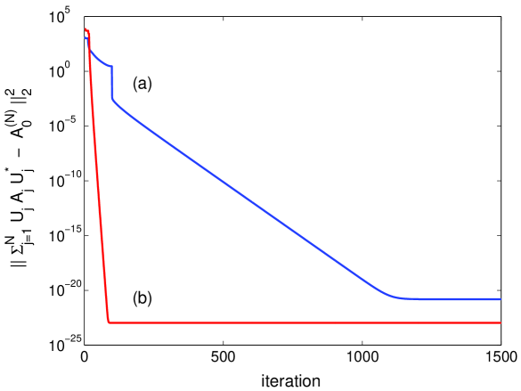
Abbildung 1: Coupled flows minimizing $||\sum_{j=1}^{N}U_{j}A_{j}U_{j}^{*}-A_{0}^{(N)}||^{2}_{2}$ with (a) $N=2$ and (b) $N=10$ for Example 1.

As shown in Fig. 1, the gradient flow of Eqn. 2.10 minimizes $||\sum_{j=1}^{N}U_{j}A_{j}U_{j}^{*}-A_{0}^{(N)}||^{2}_{2}$ by driving it practically to zero. Note that in Fig. 1b the combined flow on $N=10$ unitaries converges even faster than in Fig. 1a, where $N=2$ and the flow is more sensitive to saddle points as may be inferred from the jumps in trace (a).

Example 2
Let $A,B$ be Hermitian and $C$ arbitrary, e.g., $A=\left(\begin{smallmatrix}2&5&11\\ 5&8&15\\ 11&15&16\end{smallmatrix}\right),\;B=\left(\begin{smallmatrix}6&8&9\\ 8&12&10\\ 9&10&0\end{smallmatrix}\right),\;C=\left(\begin{smallmatrix}1&11&3\\ 6&9&3\\ 8&9&2\end{smallmatrix}\right)\;.$ Then $a:=\operatorname{eig}(A)=(-5.6674;-0.4830;32.1504),b:=\operatorname{eig}(B)=(-7.4816;0.7123;24.7693)$ and $f:=\operatorname{eig}\tfrac{1}{2}(C+C^{*})=(-4.9555;-1.3888;18.3443),g:=\operatorname{eig}\tfrac{-i}{2}(C-C^{*})=(-4.6368;0;4.6368)$. According to Theorem 2.1 one gets

$$\Delta:=\underset{U,V\in SU(3)}{\min}||UAU^{*}+iVBV^{*}-C||_{2}^{2}=(a-f)^{*}(a-f)+(b-g)^{*}(b-g)=605.8521\;.$$ (2.11)

More precisely $\Delta=605.852131091^{\prime}3004$, while 100 runs of the gradient flow with independent random initial conditions give a mean $\pm$ rmsd. of $\bar{\Delta}=605.852131091^{\prime}3570\pm 1.13\cdot 10^{-10}$.

3 Unitary Equivalence

In this section, we study

$$\min\left\{\|\sum_{j=1}^{N}U_{j}A_{j}V_{j}-A_{0}\|:U_{1},\dots,U_{N}\in U(n){\quad\text{and}\quad}V_{1},\dots,V_{N}\in U(m)\;\hbox{ unitary}\right\}$$

for rectangular matrices $A_{0},\dots,A_{N}$. By the result of O’Shea and Sjamaar [32],

$$\min\|\sum_{j=1}^{N}U_{j}A_{j}V_{j}-A_{0}\|=0$$

if and only if

$$\min\|\sum_{j=1}^{N}W_{j}^{*}\tilde{A}_{j}W_{j}-\tilde{A}_{0}\|=0$$

where

$$\tilde{A}_{j}=\begin{pmatrix}0&A_{j}\cr A_{j}^{*}&0\cr\end{pmatrix}\qquad\hbox{ for }j=0,1,\dots,N.$$

Thus, by the results concerning unitary similarity orbits (see Section 2),

$$\min\left\{\|A_{0}-\sum_{j=1}^{N}U_{j}A_{j}V_{j}\|:U_{1},\dots,U_{N};\,V_{1},\dots,V_{N}\;\hbox{ unitary}\right\}=0$$ (3.12)

if and only if the singular values of $A_{0},A_{1},\dots,A_{N}$ satisfy a certain set of linear inequalities. Clearly, $\min\left\{\|A-UBV\|:U,V\hbox{ unitary}\right\}=0$ if and only if $A$ and $B$ have the same singular values. In general, it is interesting to check whether

$$\sqrt{2}\min\|\sum_{j=1}^{N}U_{j}A_{j}V_{j}-A_{0}\|=\min\|\sum_{j=1}^{N}W_{j}^{*}\tilde{A}_{j}W_{j}-\tilde{A}_{0}\|=0.$$

In computer experiments (see Example 6 in Section 3), we observe that (3.12) always holds if $A_{0},A_{1},\dots,A_{N}$ are randomly generated matrices generated by matlab. We explain this phenomenon in the following. We begin with a simple observation.

Lemma 3.1

Suppose $a_{0},a_{1},\dots,a_{N}\in(0,\infty)$. The following are equivalent.

(a) There are complex units $e^{it_{1}},\dots,e^{it_{N}}$ such that $a_{0}-\sum_{j=1}^{N}a_{j}e^{it_{j}}=0.$

(b) There is an $N+1$ side convex polygon whose sides have lengths $a_{0},\dots,a_{N}$.

(c) $\sum_{j=0}^{N}a_{j}-2a_{k}\geq 0$ for all $k=0,1,\dots,N$.

Form this observation, one easily gets the following condition related to the equality (3.12).

Proposition 3.2

Let $A_{j}={\rm diag}\,(a_{1j},\dots,a_{nj})$ be nonnegative diagonal matrices for $j=0,1,\dots,N$, and let $v_{j}=(a_{1j},\dots,a_{nj})^{t}$. Then there exist permutation matrices $P_{1},\dots,P_{N}$ and diagonal unitary matrices $D_{1},\dots,D_{N}$ such that

$$A_{0}=\sum_{j=1}^{N}D_{j}P_{j}A_{j}P_{j}^{t}$$

if and only if the entries of each row of the matrix

$$[v_{0}|P_{1}v_{1}|\cdots|P_{N}v_{N}]$$

correspond to the sides of a $N+1$ side convex polygon.

If one examines the singular values of an $n\times n$ random matrix generated by matlab, we see that there is always a dominant singular values of size about $n/2$, and the other singular values range from 0 to $1.5n$ in a rather systematic pattern. So, it is often possible to apply Proposition 3.2 to get equality (3.12) if $A_{0},\dots,A_{N}$ are random matrices generated by matlab for $N\geq 2$.

In contrast, for general matrices, it is easy to construct $A_{0},A_{1},\dots,A_{N}$ such that (3.12) fails.

Example 3
Let $A_{0}={\rm diag}\,(N^{2},N+1)\oplus 0_{n-2}$ and $A_{j}={\rm diag}\,(N,1)\oplus 0_{n-2}$ for $j=1,\dots,N$. Then clearly Eqn. 3.12 does not apply, because

$$\sum_{j=1}^{n}s_{j}(A_{0})>\sum_{i=1}^{N}\sum_{j=1}^{n}s_{j}(A_{j}).$$

Recall that the Ky Fan $k$-norm of a matrix $A\in M_{n}$ is defined as $\|A\|_{k}=\sum_{j=1}^{k}s_{j}(A)$, and a norm $\|\cdot\|$ on $M_{n}$ is unitarily invariant if $\|A\|=\|UAV\|$ for all $A\in M_{n}$ and unitary $U,V\in M_{n}$. By the Ky Fan dominance theorem, two matrices $A,B\in M_{n}$ satisfy $\|A\|_{k}\leq\|B\|_{k}$ for $k=1,\dots,n$ if and only if $\|A\|\leq\|B\|$ for all unitarily invariant norms $\|\cdot\|$. In view of this example, we have the following result.

Proposition 3.3

Suppose $A_{0},A_{1},\dots,A_{N}\in M_{n}$ satisfy (3.12). Then for all unitarily invariant norms,

$$2\|A_{i}\|\leq\sum_{j=0}^{N}\|A_{j}\|,\qquad i=0,1,\dots,N,$$

and equivalently, for $k=1,\dots,n$,

$$2\|A_{i}\|_{k}\leq\sum_{j=0}^{N}\|A_{j}\|_{k},\qquad i=0,1,\dots,N.$$ (3.13)

Moreover, if there is $k$ such that equality (3.13) holds, then (3.12) holds if and only if $A_{j}$ is unitarily similar to $B_{j}\oplus C_{j}$ with $B_{j}\in M_{k}$ for $j=0,\dots,N$ such that

$$\min\left\{\|B_{0}-\sum_{j=1}^{N}U_{j}B_{j}V_{j}\|:U_{1},\dots,U_{N},V_{1},\dots,V_{N}\in M_{k}\hbox{ are unitary}\right\}=0$$

and

$$\min\left\{\|C_{0}-\sum_{j=1}^{N}X_{j}C_{j}Y_{j}\|:X_{1},\dots,X_{N},Y_{1},\dots,Y_{N}\in M_{n-k}\hbox{ are unitary}\right\}=0.$$

It would be nice if one can get (3.12) by checking the relatively easy condition (3.13). Unfortunately, the following example shows that it is not true.

Example 4
Let $A_{0}={\rm diag}\,(14,2)$, $A_{1}={\rm diag}\,(8,0)$, $A_{2}={\rm diag}\,(7,4)$. Then (3.13) is satisfied for all $k\geq 1$ but by the result in [23],

$${\rm diag}\,\left(U_{1}A_{1}V_{1}+U_{2}A_{2}V_{2}\right)\neq(14,2)$$

for all unitaries $U_{i},\ V_{j}$.

3.1 Deriving Gradient Flows on Unitary Equivalence Orbits

For minimizing $||UAV-C||_{2}^{2}$ one has to maximize

$$F(U,V):=\operatorname{Re}{\rm tr}\,\left\{UAVC^{*}\right\}=\tfrac{1}{2}{\rm tr}\,\left\{UAVC^{*}+(UAVC^{*})^{*}\right\}\;.$$

By the same arguments as before, from its Fréchet differential

$$D_{U}F(U,V)(\Omega U)=\tfrac{1}{2}{\rm tr}\,\left\{(\Omega U)AVC^{*}-CV^{*}A^{*}U^{*}(\Omega U)U^{*}\right\}=\tfrac{1}{2}{\rm tr}\,\left\{(AVC^{*}-U^{*}CV^{*}A^{*}U^{*})(\Omega U)\right\}$$

one obtains the gradient—where henceforth we keep writing $(\cdot)_{s}$ for the skew-Hermitian part

$$\operatorname{grad}_{U}F(U,V)=\tfrac{1}{2}(AVC^{*}-U^{*}CV^{*}A^{*}U^{*})^{*}=-(UAVC^{*})_{s}\;U\;.$$

An analogous result follows for $\operatorname{grad}_{V}F(U,V)$. Taking again the respective Riemannian exponentials leads to the recursive scheme

$$U_{k+1} = \exp\left\{-\alpha_{k}(U_{k}AV_{k}C^{*})_{s}\right\}\;U_{k}$$

$$V_{k+1} = \exp\left\{-\beta_{k}(V_{k}C^{*}U_{k}A)_{s}\right\}\;V_{k}\;,$$

which also can be used, e.g., for a singular-value decomposition of $A$ by choosing $C$ real diagonal.

Likewise, minimizing $||UAV+XBY-C||^{2}_{2}$ by maximizing $\operatorname{Re}{\rm tr}\,\left\{UAV(C-XBY)^{*}+XBYC^{*}\right\}$ translates into the same flows when substituting $C\mapsto(C-X_{k}BY_{k})$ with analogous recursions for $X_{k+1}$ and $Y_{k+1}$. Along these lines, it is straightforward to address the general task

$$\min\left\{\|\sum_{j=1}^{N}U_{j}A_{j}V_{j}-A_{0}\|:U_{1},\dots,U_{N}\in U(n){\quad\text{and}\quad}V_{1},\dots,V_{N}\in U(m)\;\hbox{ unitary}\right\}$$ (3.14)

with rectangular matrices $A_{0},\dots,A_{N}$ by a system of $2N$ coupled gradient flows ($j=1,2,\dots,N$)

$$U_{k+1}^{(j)} = \exp\left\{-\alpha_{k}^{(j)}(U_{k}^{(j)}A_{j}V_{k}^{(j)}A_{0jk}^{*})_{s}\right\}\;U_{k}^{(j)}$$ (3.15)

$$V_{k+1}^{(j)} = \exp\left\{-\beta_{k}^{(j)}(V_{k}^{(j)}A_{0jk}^{*}U_{k}^{(j)}A_{j})_{s}\right\}\;V_{k}^{(j)}$$ (3.16)

where we use the short-hand $A_{0jk}:=A_{0}-\sum\limits_{\nu=1\atop\nu\neq j}^{N}U_{k}^{(\nu)}A_{\nu}V_{k}^{(\nu)}$.

3.2 Numerical Examples

Using the flows derived in section 3.1, in this section, we study

$$\min\left\{\|\sum_{j=1}^{N}U_{j}A_{j}V_{j}-A_{0}\|:U_{1},\dots,U_{N}\in U(n){\quad\text{and}\quad}V_{1},\dots,V_{N}\in U(m)\hbox{ unitary}\right\}$$

for rectangular matrices $A_{0},\dots,A_{N}$.

Example 5
As an example of rectangular $A_{j}\in{\mathbf{C}}^{10\times 15}$, consider the analogous flows. In order to obtain $U_{j}\in{\mathbf{C}}^{10\times 10}$ and $V_{j}\in{\mathbf{C}}^{15\times 15}$ for $j=1,2,\dots,N$ choose a set of random unitary pairs $(U_{j}^{(r)},V_{j}^{(r)})\in{\mathbf{C}}^{10\times 10}\times{\mathbf{C}}^{15\times 15}$ and define

$$A_{j}:=[\,{\rm diag}\,(1,3,5,\dots,19)+\tfrac{j-1}{10}{\rm 1\negthickspace l}{}_{10}\;|\;\mathbb{O}{}_{10,5}\,]\quad\text{and}\quad A_{0}^{(N)}:=[\,{\rm diag}\,(s_{1},...,s_{10})\;|\;\mathbb{O}{}_{10,5}\,]$$

where $s_{1},s_{2},\dots,s_{10}$ are now the singular values of $A^{\prime}_{0,N}:=\sum_{j=1}^{N}U_{j}^{(r)}A_{j}V_{j}^{(r)}$ and $\mathbb{O}{}_{10,5}$ is the $10\times 5$ zero-matrix.

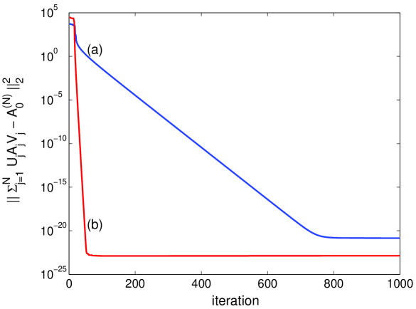
Abbildung 2: Coupled flows minimizing $||\sum_{j=1}^{N}U_{j}A_{j}V_{j}-A_{0}^{(N)}||^{2}_{2}$ with (a) $N=2$ and (b) $N=10$. Here the $A_{j}\in{\mathbf{C}}^{10\times 15}$ are rectangular so that $U_{j}\in{\mathbf{C}}^{10\times 10}$ and $V_{j}\in{\mathbf{C}}^{15\times 15}$.

Fig. 2 shows how the coupled gradient flow minimizes $||\sum_{j=1}^{N}U_{j}A_{j}V_{j}-A_{0}^{(N)}||^{2}_{2}$ by driving it practically to zero. Again the combined flow on $N=10$ unitary pairs (Fig. 2b) converges faster than the one for $N=2$ unitary pairs given in Fig. 2a.

3.2.1 Observation Concerning Sums of Unitary Equivalence Orbits

A non-zero random complex matrix $A_{0}$ is typically distant from a single equivalence orbit of another (non-zero) random matrix $UA_{1}V$ of the same dimension, since generically $A_{0}$ and $A_{1}$ clearly do not share the same singular values. However, a random complex matrix $A_{0}$ is in fact typically arbitrarily close to a sum of two or more equivalence orbits of independent random matrices. This is shown in Fig. 3 by a numerical example for $10\times 10$ complex square matrices, where the inset shows this does not hold for similarity orbits of random square matrices. Interestingly, the findings hold independent of the dimensions and explicitly include rectangular matrices as well as square matrices.

Example 6
For a single random complex square matrix $A_{0}\in{\mathbf{C}}^{10\times 10}$ we now ask how close it typically is to the sum of $N=1,2,3,4,5,10$ equivalence orbits $\sum_{j=1}^{N}U_{j}A_{j}V_{j}$, where the $A_{j}$ are independently chosen random complex matrices $A_{j}\in{\mathbf{C}}^{10\times 10}$. We compare the findings with those of $N$ independent similarity orbits $\sum_{j=1}^{N}U_{j}A_{j}U^{*}_{j}$ and find the results of Fig. 3 underscoring Proposition 3.2.

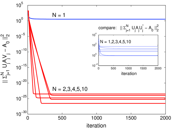
Abbildung 3: A random complex square matrix $A_{0}\in{\mathbf{C}}^{10\times 10}$ is typically distant from a single ($N=1$) equivalence orbit of another random square matrix $UA_{1}V$, as shown in the upper trace. However, it is typically arbitrarily close to a sum of equivalence orbits of several independent random square matrices as demonstrated in the lower traces: $\|\sum_{j=1}^{N}U_{j}A_{j}V_{j}-A_{0}\|^{2}_{2}\to 0$ for $N=2,3,4,5,10$. In contrast, the inset shows this does not hold for $N=1$ through $N=10$ for similarity orbits $\sum_{j=1}^{N}U_{j}A_{j}U^{*}_{j}$.

4 Unitary $t$-Congruence

In this section, we consider

$$\min\left\{\|\sum_{j=1}^{N}U_{j}A_{j}U_{j}^{t}-A_{0}\|:U_{1},\dots,U_{N}\in U(n)\hbox{ unitary}\right\}$$

for given matrices $A_{0},A_{1},\dots,A_{N}$. Sometimes, we can focus on special classes of matrices such as symmetric matrices or skew-symmetric matrices. For symmetric matrices or skew-symmetric matrices, the minimization problem

$$\min\left\{\|UAU^{t}-A_{0}\|:U\hbox{ unitary}\right\}$$

has an analytic solution; see [26]. The problem is wide open even if $N=2$. Therefore, a computer algorithm will be most helpful in the theoretical development. One may also consider whether we can have $UAU^{t}+VBV^{t}=C$ for a symmetric $A$ and a skew-symmetric $B$. In other words, we want to know whether one can write $C$ as the sum of symmetric and skew-symmetric matrices with prescribed singular values. Of course, the problem for general matrices $A,B$ and $C$ is even more challenging, and that is what we pursue by the numerical methods developed in the next paragraph.

4.1 Gradient Flows on Unitary $t$-Congruence Orbits

Again, the minimization task

$$\underset{U,V\in U(n)}{\min}||UAU^{t}+VBV^{t}-C||_{2}^{2}\;,$$ (4.17)

translates via

$$||UAU^{t}+VBV^{t}-C||_{2}^{2}\\ =||A||_{2}^{2}+||B||_{2}^{2}+||C||_{2}^{2}-2\operatorname{Re}{\rm tr}\,\left\{C^{*}(UAU^{t}+VBV^{t})-UAU^{t}\;\bar{V}B^{*}V^{*}\right\}$$

into maximising the function

$$F(U,V):=\operatorname{Re}f(U,V):=\operatorname{Re}{\rm tr}\,\left\{(UAU^{t}+VBV^{t})\,C^{*}-UAU^{t}\;\bar{V}B^{*}V^{*}\right\}\quad,$$ (4.18)

where the differential reads (by virtue of the short-hand $\tilde{C}:=C^{*}-\bar{V}B^{*}V^{*}$)

$$D_{U}f(U)(\Omega U) = {\rm tr}\,\left\{((\Omega U)AU^{t}+UA(\Omega U)^{t})(C^{*}-\bar{V}B^{*}V^{*})\right\}$$

$$= {\rm tr}\,\left\{(\Omega U)AU^{t}\tilde{C}\right\}+{\rm tr}\,\left\{(UA(\Omega U)^{t}\tilde{C})^{t}\right\}$$

$$= {\rm tr}\,\left\{(AU^{t}\tilde{C}+A^{t}U^{t}\tilde{C}^{t})(\Omega U)\right\}\quad.$$

From identifying $D_{U}f(U)\cdot(\Omega U)=\langle\operatorname{grad}_{U}f(U)|\Omega U\rangle{}={\rm tr}\,\left\{(\operatorname{grad}_{U}f(U))^{*}\Omega U\right\}$ one finds

$$\operatorname{grad}_{U}f(U)=(UAU^{t}\tilde{C}+UA^{t}U^{t}\tilde{C}^{t})^{*}U$$ (4.19)

so as to obtain for $F(U):=\operatorname{Re}f(U)$

$$\operatorname{grad}_{U}F(U)=-\big{(}UAU^{t}\tilde{C}+UA^{t}U^{t}\tilde{C}^{t}\big{)}_{s}\,U\quad.$$ (4.20)

Again, taking the respective Riemannian exponentials $\exp_{U}(\operatorname{grad}_{U}F(U))$ and $\exp_{V}(\operatorname{grad}_{V}F(V))$ thus gives the slightly lengthy formula

$$U_{k+1}=\exp\left\{-\alpha_{k}\big{(}U_{k}AU_{k}^{t}(C^{*}-\bar{V}_{k}B^{*}V_{k}^{*})+U_{k}A^{t}U_{k}^{t}(C^{*}-\bar{V}_{k}B^{*}V_{k}^{*})^{t}\big{)}_{s}\right\}\;U_{k}$$ (4.21)

—and an analogous equation for $V_{k+1}$ by substituting $V$ for $U$ and $B$ for $A$—as discretized solutions of the coupled gradient system

$$\dot{U}=\operatorname{grad}_{U}F(U,V)\quad\text{\rm and}\quad\dot{V}=\operatorname{grad}_{V}F(U,V)\;.$$ (4.22)

Likewise, for higher sums of congruence orbits one finds

$$\min\left\{\|\sum_{j=1}^{N}U_{j}A_{j}U^{t}_{j}-A_{0}\|:U_{1},\dots,U_{N}\in U(n)\;\hbox{ unitary}\right\}$$ (4.23)

to be solved by the coupled system of flows ($j=1,2,\dots,N$)

$$U_{k+1}^{(j)}=\exp\left\{-\alpha_{k}^{(j)}{\big{(}A_{k}^{(j)}A_{0jk}^{*}+(A_{0jk}^{*}A_{k}^{(j)})^{t}\big{)}}_{s}\right\}\;U_{k}^{(j)}\quad,$$ (4.24)

where for short we set $A_{k}^{(j)}:=U_{k}^{(j)}A_{j}{U_{k}^{{}^{t}(j)}}$ and $A_{0jk}:=A_{0}-\sum\limits_{\nu=1\atop\nu\neq j}^{N}A_{k}^{(\nu)}$.

5 Outlook: Non-Compact Groups

For orbits $S(A)$ of matrices $A$ under the action of non-compact groups, there are usually no good results for supremum or infinmum of the quantity

$$\|X_{0}-\sum_{j=1}^{N}X_{j}\|$$

with $X_{j}\in S(A_{j})$ for $j=0,1,\dots,N$, for given matrices $A_{0},\dots,A_{N}$.

For example, for the invertible congruence orbit of $A\in M_{n}$

$$S(A)=\left\{S^{*}AS:S\in M_{n}\hbox{ is invertible}\right\},$$

we can let $S=rI$. Then

$$\|S^{*}A_{0}S-\sum_{j=1}^{N}S^{*}A_{j}S\|$$

converges to 0 or $\infty$ depending on $r\rightarrow 0$ or $r\rightarrow\infty$.

Similarly, the same problems occur for the equivalence orbit of $A\in M_{n}$

$$S(A)=\left\{SAT:S,T\in M_{n}\hbox{ are invertible}\right\}.$$

For the similarity orbits, we have the following.

Proposition 5.1

Suppose not all the matrices $A_{0},\dots,A_{N}$ are scalar. Then

$$\sup\|A_{0}-\sum_{j=1}^{N}S_{j}^{-1}A_{j}S_{j}\|=\infty.$$

Proof. Suppose one of the matrices, say, $A_{i}$ is non-scalar. Then there is $S_{j}$ such that $S_{j}^{-1}A_{i}S_{j}$ is in lower triangular form with the $(2,1)$ entry equal to 1, and there are invertible matrices $S_{j}$ such that $S_{j}^{-1}A_{j}s_{j}$ is in upper triangular form for other $j$. Let $D_{r}={\rm diag}\,(r,1,1,\dots,1)$. Then the sequence

$$(S_{0}D_{r})^{-1}A_{0}(S_{0}D_{r})-\sum_{j=1}^{N}(S_{j}D_{r})^{-1}A_{j}(S_{j}D_{r})$$

has unbounded $(2,1)$ entry as $r\rightarrow\infty$. The conclusion follows.   

Determining

$$\inf\|A_{0}-\sum_{j=1}^{N}S_{j}^{-1}A_{j}S_{j}\|$$

is more challenging. Let us first consider two matrices $A,B\in M_{n}$. We have the following.

Proposition 5.2

Let $A,B\in M_{n}$. Then for any unitary similarity invariant norm $\|\cdot\|$,

$$\|({\rm tr}\,A-{\rm tr}\,B)I/n\|\leq\|S^{-1}AS-T^{-1}BT\|$$

for any invertible $S$ and $T$.

Proof. Given two real vectors $x=(x_{1},\dots,x_{n}),y=(y_{1},\dots,y_{n})$, we say that $x$ is weakly majorized by $y$, denoted by $x\prec_{w}y$ if the sum of the $k$ largest entries of $x$ is not larger than that of $y$ for $k=1,\dots,n$. By the Ky Fan dominance theorem, if $X={\rm diag}\,(x_{1},\dots,x_{n})$ and $Y={\rm diag}\,(y_{1},\dots,y_{n})$ are nonnegative matrices such that $(x_{1},\dots,x_{n})\prec_{w}(y_{1},\dots,y_{n})$, then $\|X\|\leq\|Y\|$ for any unitarily invariant norm $\|\cdot\|$.

Now, suppose $S^{-1}AS-T^{-1}BT$ has diagonal entries $d_{1},\dots,d_{n}$ and singular values $s_{1},\dots,s_{n}$. Then

$$|{\rm tr}\,A-{\rm tr}\,B|=|\sum_{j=1}^{n}d_{j}|\leq\sum_{j=1}^{n}|d_{j}|.$$

Thus,

$$|{\rm tr}\,A-{\rm tr}\,B|(1,\dots,1)/n\prec_{w}(|d_{1}|,\dots,|d_{n}|)\prec_{w}(s_{1},\dots,s_{n}).$$

It follows that

$$\|({\rm tr}\,A-{\rm tr}\,B)I/n\|\leq\|{\rm diag}\,(|d_{1}|,\dots,|d_{n}|)\leq\|{\rm diag}\,(s_{1},\dots,s_{n})\|=\|S^{-1}AS-T^{-1}BT\|.$$

  

Can we always find invertible $S$ and $T$ such that

$$\|S^{-1}AS-T^{-1}BT\|=\|({\rm tr}\,A-{\rm tr}\,B)I/n\|?$$

The answer is no, and we have the following.

Proposition 5.3

Let $\|\cdot\|$ be a unitarily invariant norm on $M_{n}$. Suppose $A\in M_{n}$ has eigenvalues $a_{1},\dots,a_{n}$, and $B=bI$. Then

$$\inf\left\{\|S^{-1}AS-B\|:S\in M_{n}\hbox{ is invertible}\right\}=\|{\rm diag}\,(a_{1}-b,\dots,a_{n}-b)\|.$$

Proof. Suppose $S^{-1}AS-B$ has eigenvalues $a_{1}-b,\dots,a_{n}-b$, and singular values $s_{1},\dots,s_{n}$. Then the product of the $k$ largest entries of the vector $(|a_{1}-b|,\dots,|a_{n}-b|)$ is not larger than $(s_{1},\dots,s_{n})$ for $k=1,\dots,n$. It follows that

$$(|a_{1}-b|,\dots,|a_{n}-b|)\prec_{w}(s_{1},\dots,s_{n}),$$

and hence

$$\|{\rm diag}\,(|a_{1}-b|,\dots,|a_{n}-b|)\|\leq\|{\rm diag}\,(s_{1},\dots,s_{n})\|=\|S^{-1}AS-B\|.$$

Note that there is $S$ such that $S^{-1}(A-B)S$ is in upper triangular Jordan form with diagonal entries $a_{1}-b,\dots,a_{n}-b$. Let $D_{r}={\rm diag}\,(1,r,\dots,r^{n-1})$ for $r>0$. Then $(SD_{r})^{-1}(A-B)(SD_{r})\rightarrow{\rm diag}\,(a_{1}-b,\dots,a_{n}-b)$ and $\|(SD_{r})^{-1}(A-B)(SD_{r})\|\rightarrow\|{\rm diag}\,(a_{1}-b,\dots,a_{n}-b)\|$ as $r\rightarrow 0$. So, we get the conclusion about the infinmum.   

From the above result and proof, we see that if $A$ has an eigenvalue $a$ with eigenspace of dimension $p$ and $B$ has an eigenvalue $b$ with eigenspace of dimension $q$ such that $p+q-n=r>0$ then $S^{-1}AS-T^{-1}BT$ has an eigenvalue $a-b$ of multiplicity at least $r$. The question is whether we can write $A=aI_{r}\oplus A_{1}$ and $B=bI_{r}\oplus B_{1}$ and show that

$$\inf\|S_{1}^{-1}A_{1}S_{1}-T_{1}^{-1}B_{1}T_{1}\|=\|({\rm tr}\,A_{1}-{\rm tr}\,B_{1})I_{n-k}/(n-k)\|.$$

It is interesting to note that the following two quantities may be different.

1) $\inf\left\{\|S^{-1}AS-T^{-1}BT\|:S\hbox{ is invertible}\right\}$.

2) $\inf\left\{\|S^{-1}AS-B\|:S\hbox{ is invertible}\right\}$.

For example, suppose $A={\rm diag}\,(2,-1,-1)$ and $B=\left(\begin{array}[]{ccc}0&1&0\\ 0&0&1\\ 0&0&0\end{array}\right)$. Then there are invertible $S$ and $T$ such that

$$S^{-1}AS=\begin{pmatrix}0&1&1\\ 1&0&1\\ 1&1&0\cr\end{pmatrix}\quad\hbox{ and }\quad T^{-1}BT=\begin{pmatrix}0&1&1\\ 0&0&1\\ 0&0&0\cr\end{pmatrix}.$$

So, $C=S^{-1}AS-T^{-1}BT$ is a rank two nilpotent. Thus for any $\varepsilon>0$, there is an invertible $R_{\varepsilon}$ such that

$$R_{\varepsilon}^{-1}CR_{\varepsilon}=\begin{pmatrix}0&\varepsilon&0\\ 0&0&\varepsilon\\ 0&0&0\cr\end{pmatrix}.$$

As a result,

$$\|R_{\varepsilon}^{-1}S^{-1}ASR_{\varepsilon}-R_{\varepsilon}^{-1}T^{-1}BTR_{\varepsilon}\|\rightarrow 0\quad\hbox{ as }\quad\varepsilon\rightarrow 0.$$

So, the quantity in (1) equals zero. On the other hand, for every invertible $S$, we have

$$\|\left(A-SBS^{-1}\right)\left(Se_{1}\right)\|=\|A\left(Se_{1}\right)\|\geq\|Se_{1}\|$$

Therefore, $\inf\|A-SBS^{-1}\|\geq 1$. So, we see that the quantities in (1) and (2) may be different.

In connection to the above discussion, it is interesting to study the following problem.

1. Determine

$$\inf\left\{\|S^{-1}AS-TBT^{-1}\|:S,T\hbox{ are invertible}\right\}$$

and characterize the matrix pairs $(A,B)$

2. Determine

$$\inf\left\{\|S^{-1}AS-B\|:S\hbox{ is invertible}\right\}$$

and characterize the matrix pairs $(A,B)$ attaining the infinmum if they exist.

6 Conclusions

We have treated the least-squares approximation problems by elements on the sum of various matrix orbits including unitary similarity, equivalence and congruence. Special attention has been paid to sums of unitary similarity orbits of a Hermitian $A$ and a skew-Hermitian $B$, where theoretical results have been obtained and shown to be consistent with numerical findings. Further, new results on unitary equivalence orbits have been obtained stimulated by numerical experiments. are related to geometric arguments.

A general framework based on the gradient flows on matrix orbits arising from Lie group actions has been developed to study the proposed problems. The gradient flows devised to this end extend the existing toolbox (see e.g. [2, 9]) by referring to sums of matrix orbits as summerized in Tab. 1. This general approach can be used to treat many problems in theory and applications. For instance, flows on such sums of unitary similarity orbits can also be envisaged as on unitaries taking a block-diagonal form, and hence they relate to relative $C$ numerical ranges, where the group action is restricted to a compact subgroup $\mathbf{K}\subseteq SU(n)$ of the full unitary group [29]. Finally, first results on matrix orbits under non-compact group actions invite further research.

Tabelle 1: Summary of Least-Squares Approximations by Matrix Orbits and Related Gradient Flows

type  and  objective		coupled gradient flows
unitary similarity:
$\underset{U\in SU(n)}{\min}=\|\sum\limits_{j=1}^{N}U_{j}A_{j}U^{*}_{j}-A_{0}\|$		$U_{k+1}^{(j)}=\exp\left\{-\alpha_{k}^{(j)}{[A_{k}^{(j)},A_{0jk}^{*}]}_{s}\right\}\;U_{k}^{(j)}$
		where   $A_{k}^{(j)}:=U_{k}^{(j)}A_{j}{U_{k}^{(j)}}^{*}$ and $A_{0jk}:=A_{0}-\sum\limits_{\nu=1\atop\nu\neq j}^{N}A_{k}^{(\nu)}$
unitary equivalence:
$\underset{U,V\in SU(n)}{\min}\|\sum\limits_{j=1}^{N}U_{j}A_{j}V_{j}-A_{0}\|$		$U_{k+1}^{(j)}=\exp\left\{-\alpha_{k}^{(j)}(U_{k}^{(j)}A_{j}V_{k}^{(j)}A_{0jk}^{*})_{s}\right\}\;U_{k}^{(j)}$
		$V_{k+1}^{(j)}=\exp\left\{-\beta_{k}^{(j)}(V_{k}^{(j)}A_{0jk}^{*}U_{k}^{(j)}A_{j})_{s}\right\}\;V_{k}^{(j)}$
		where   $A_{0jk}:=A_{0}-\sum\limits_{\nu=1\atop\nu\neq j}^{N}U_{k}^{(\nu)}A_{\nu}V_{k}^{(\nu)}$
unitary congruence:
$\underset{U\in SU(n)}{\min}\|\sum\limits_{j=1}^{N}U_{j}A_{j}U^{t}_{j}-A_{0}\|$		$U_{k+1}^{(j)}=\exp\left\{-\alpha_{k}^{(j)}{\big{(}A_{k}^{(j)}A_{0jk}^{*}+(A_{0jk}^{*}A_{k}^{(j)})^{t}\big{)}}_{s}\right\}\;U_{k}^{(j)}$
		where   $A_{k}^{(j)}:=U_{k}^{(j)}A_{j}{U_{k}^{(j)}}^{t}$ and $A_{0jk}:=A_{0}-\sum\limits_{\nu=1\atop\nu\neq j}^{N}A_{k}^{(\nu)}$

7 Further Research

In order to avoid the search in our algorithms is terminated in local extrema, one has to ensure to choose a sufficiently large set of random unitaries distributed according to the Haar measure. Actually, one knows there are commutation properties at the critical points. It would be nice to find a more efficient method to choose starting points for the search, and prove theorems ensuring that the absolute minimum will be reached from one of these starting points using our algorithms.

Our discussion focused on orbits of matrices under actions of compact groups. We can consider other orbits under actions of non-compact groups. Here are some examples for $S,T\in SL(n,{\mathbf{C}})$:

(e) the general similarity orbit of a square matrix $A$ is the set of matrices of the form $SAS^{-1}$,

(f) the equivalence orbit of a rectangular matrix $A$ is the set of matrices of the form $SAT$,

(g) the $*$-congruence orbit of a complex square matrix $A$ is the set of matrices of the form $SAS^{*}$,

(h) the $t$-congruence orbit of a square matrix $A$ is the set of matrices of the form $SAS^{t}$.

However, the fact that $GL(n,{\mathbf{C}})$ and $SL(n,{\mathbf{C}})$ are just locally compact entails there is no Haar measure and consequently no bi-invariant metric on the tangent spaces, but only left or right-invariant metrics. Hence the Hilbert-Schmidt scalar product $\langle B|A\rangle{}={\rm tr}\,\left\{B^{*}A\right\}$ has to be treated with care, in particular since we are interested in the complex domain. Moreover, while in compact Lie groups the exponential map is surjective and geodesic [1], in locally compact Lie groups, it is generically neither surjective nor geodesic. It is for these reasons that devising gradient flows in locally compact Lie groups is the subject of a follow-up study.

• [1] A. Arvanitoyeorgos, An Introduction to Lie Groups and the Geometry of Homogeneous Spaces, American Mathematical Society, Providence, 2003: especially p 125 ff.
• [2] A. Bloch, Ed., Hamiltonian and Gradient Flows, Algorithms and Control, Fields Institute Communications, American Mathematical Society, Providence, 1994.
• [3] R.W. Brockett, Dynamical Systems that Sort Lists, Diagonalise Matrices, and Solve Linear Programming Problems. In Proc. IEEE Decision Control, 1988, Austin, Texas, pages 779–803, 1988; reproduced in: Linear Algebra Appl. 146 (1991), 79–91.
• [4] A.S. Buch, The Saturation Conjecture (after A. Knutson and T. Tao) with an Appendix by William Fulton, Enseign. Math. 46 (2000), 43–60.
• [5] C.M. Cheng, R.A. Horn, and C.K. Li, Inequalities and Equalities for the Cartesian Decomposition, Linear Algebra Appl. 341 (2002), 219–237.
• [6] M.D. Choi and P.Y. Wu, Convex Combinations of Projections, Linear Algebra Appl. 136 (1990), 25–42.
• [7] M.D. Choi and P.Y. Wu, Finite-Rank Perturbations of Positive Operators and Isometries, Studia Math. 173 (2006), no. 1, 73–79.
• [8] M. Christandl, A Quantum Information-Theoretic Proof of the Relation between Horn’s Problem and the Littlewood-Richardson Coefficients, Lecture Notes in Computer Science 5028 (2008), 120–128.
• [9] M. T. Chu, F. Diele, and I. Sgura, Gradient Flow Methods for Matrix Completion with Prescribed Eigenvalues, Linear Algebra and its Applications, 379 (2004), 85–112 .
• [10] J. Day, W. So and R.C. Thompson, The Spectrum of a Hermitian Matrix Sum, Linear Algebra Appl. 280 (1998), 289–332.
• [11] K. Fan and G. Pall, Imbedding Conditions for Hermitian and Normal Matrices, Canad. J. Math. 9 (1957), 298–304.
• [12] W. Fulton, Eigenvalues, Invariant Factors, Highest Weights, and Schubert Calculus, Bull. Amer. Math. Soc. 37 (2000), 209–249.
• [13] S. J. Glaser, T. Schulte-Herbrüggen, M. Sieveking, O. Schedletzky, N. C. Nielsen, O. W. Sørensen, and C. Griesinger, Unitary Control in Quantum Ensembles: Maximising Signal Intensity in Coherent Spectroscopy, Science 280 (1998), 421–424.
• [14] U. Helmke, K. Hüper, J. B. Moore, and T. Schulte-Herbrüggen. Gradient Flows Computing the $C$-Numerical Range with Applications in NMR Spectroscopy, J. Global Optim. 23 (2002), 283–308.
• [15] U. Helmke and J. B. Moore, Optimisation and Dynamical Systems. Springer, Berlin, 1994.
• [16] A. Horn, Eigenvalues of Sums of Hermitian Matrices, Pacific J. Math. 12 (1962), 225–241.
• [17] R.A. Horn and C.R. Johnson, Matrix Analysis, Cambridge University Press, New York, 1985.
• [18] A.A. Klyachko, Stable Bundles, Representation Theory and Hermitian Operators, Selecta Math. (N.S.) 4 (1998), 419–445.
• [19] A. Knutson and T. Tao, The Honeycomb Model of ${\rm GL}_{n}(\mathbb{C})$ Tensor Products. I. Proof of the Saturation Conjecture, J. Amer. Math. Soc. 12 (1999), 1055–1090.
• [20] A. Knutson and T. Tao, Honeycombs and Sums of Hermitian Matrices, Notices Amer. Math. Soc. 48 (2001), 175–185.
• [21] T.G. Lei, Congruence Numerical Ranges and Their Radii, Linear and Multilinear Algebra 43 (1998), 411–427.
• [22] C.K. Li, $C$-Numerical Ranges and $C$-Numerical Radii, Linear and Multilinear Algebra 37 (1994), 51–82.
• [23] C. K. Li and Y. T. Poon, Diagonals and Partial Diagonals of Sum of Matrices, Canadian J. Math. 54 (2002), 571–594.
• [24] C.K. Li and N.K. Tsing, On Unitarily Invariant Norms and Related Results, Linear and Multilinear Algebra 20 (1987), 107–119.
• [25] E. Marques de Sá, On the Inertia of Sums of Hermitian Matrices, Linear Algebra Appl. 37 (1981), 143–159.
• [26] A.W. Marshall and I. Olkin, Inequalities: Theory of Majorization and its Applications, Mathematics in Science and Engineering, 143. Academic Press, Inc., New York-London, 1979.
• [27] F. Mezzadri, How to Generate Random Matrices from the Classical Compact Groups, Notices of the AMS 54 (2007), 592–604.
• [28] L. Mirsky, Symmetric Gauge Functions and Unitarily Invariant Norms, Quart. J. Math. Oxford 11 (1960), 50–59.
• [29] T. Schulte-Herbrüggen, G. Dirr, U. Helmke and S. Glaser The Significance of the $C$-Numerical Range and the Local $C$-Numerical Range in Quantum Control and Quantum Information, Lin. Multilin. Alg. 56 (2008), 3–26.
• [30] T. Schulte-Herbrüggen, G. Dirr, U. Helmke and S. Glaser Gradient Flows for Optimisation and Quantum Control: Foundations and Applications, e-print: http://arxiv.org/pdf/0802.4195 (2008).
• [31] H. Shapiro, A Survey of Canonical Forms and Invariants for Unitary Similarity, Linear Algebra Appl. 147 (1991), 101–167.
• [32] L. O’Shea and R. Sjamaar, Moment Maps and Riemannian Symmetric Pairs, Math. Ann. 317 (2000), 415–457.
• [33] R.C. Thompson and L.J. Freede, On the Eigenvalues of Sums of Hermitian Matrices, Linear Algebra and Appl. 4 (1971) 369–376.
• [34] R.C. Thompson and L.J. Freede, On the Eigenvalues of Sums of Hermitian Matrices, II. Aequationes Math 5 (1970), 103–115
• [35] R.C. Thompson, Singular Values and Diagonal Elements of Complex Symmetric Matrices, Linear Algebra Appl. 26 (1979), 65–106.
• [36] R.C. Thompson, The Congruence Numerical Range, Linear and Multilinear Algebra 8 (1979/80), 197–206.
• [37] H. Weyl, Das asymptotische Verteilungsgesetz der Eigenwerte linearer partieller Differentialgleichungen, Math. Ann. 71 (1912), 441–479