Uniqueness of Brownian motion on Sierpinski carpets

Abstract

We prove that, up to scalar multiples, there exists only one local regular Dirichlet form on a generalized Sierpinski carpet that is invariant with respect to the local symmetries of the carpet. Consequently for each such fractal the law of Brownian motion is uniquely determined and the Laplacian is well defined.

1 Introduction

The standard Sierpinski carpet $F_{\rm SC}$ is the fractal that is formed by taking the unit square, dividing it into 9 equal subsquares, removing the central square, dividing each of the 8 remaining subsquares into 9 equal smaller pieces, and continuing. In [3] two of the authors of this paper gave a construction of a Brownian motion on $F_{\rm SC}$. This is a diffusion (that is, a continuous strong Markov process) which takes its values in $F_{\rm SC}$, and which is non-degenerate and invariant under all the local isometries of $F_{\rm SC}$.

Subsequently, Kusuoka and Zhou in [30] gave a different construction of a diffusion on $F_{\rm SC}$, which yielded a process that, as well as having the invariance properties of the Brownian motion constructed in [3], was also scale invariant. The proofs in [3, 30] also work for fractals that are formed in a similar manner to the standard Sierpinski carpet: we call these generalized Sierpinski carpets (GSCs). In [5] the results of [3] were extended to GSCs embedded in ${\mathbb{R}}^{d}$ for $d\geq 3$. While [3, 5] and [30] both obtained their diffusions as limits of approximating processes, the type of approximation was different: [3, 5] used a sequence of time changed reflecting Brownian motions, while [30] used a sequence of Markov chains.

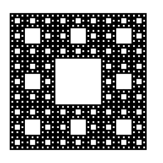
Figure 1: The standard Sierpinski carpet

These papers left open the question of uniqueness of this Brownian motion – in fact it was not even clear whether or not the processes obtained in [3, 5] or [30] were the same. This uniqueness question can also be expressed in analytic terms: one can define a Laplacian on a GSC as the infinitesimal generator of a Brownian motion, and one wants to know if there is only one such Laplacian. The main result of this paper is that, up to scalar multiples of the time parameter, there exists only one such Brownian motion; hence, up to scalar multiples, the Laplacian is uniquely defined.

GSCs are examples of spaces with anomalous diffusion. For Brownian motion on ${\mathbb{R}}^{d}$ one has ${\mathbb{E}}|X_{t}-X_{0}|=ct^{1/2}$. Anomalous diffusion in a space $F$ occurs when instead one has ${\mathbb{E}}|X_{t}-X_{0}|=o(t^{1/2})$, or (in regular enough situations), ${\mathbb{E}}|X_{t}-X_{0}|\approx t^{1/d_{w}}$, where $d_{w}$ (called the walk dimension) satisfies $d_{w}>2$. This phenomena was first observed by mathematical physicists working in the transport properties of disordered media, such as (critical) percolation clusters – see [1, 37]. Since these sets are subsets of the lattice ${\mathbb{Z}}^{d}$, they are not true fractals, but their large scale structure still exhibits fractal properties, and the simple random walk is expected to have anomalous diffusion.

For critical percolation clusters (or, more precisely for the incipient infinite cluster) on trees and ${\mathbb{Z}}^{2}$, Kesten [23] proved that anomalous diffusion occurs. After this work, little progress was made on critical percolation clusters until the recent papers [7, 8, 27].

As random sets are hard to study, it was natural to begin the study of anomalous diffusion in the more tractable context of regular deterministic fractals. The simplest of these is the Sierpinski gasket. The papers [1, 37] studied discrete random walks on graph approximations to the Sierpinski gasket, and soon after [19, 29, 11] constructed Brownian motions on the limiting set. The special structure of the Sierpinski gasket makes the uniqueness problem quite simple, and uniqueness of this Brownian motion was proved in [11]. These early papers used a probabilistic approach, first constructing the Brownian motion $X$ on the space, and then, having defined the Laplacian $\mathcal{L}_{X}$ as the infinitesimal generator of the semigroup of $X$, used the process $X$ to study $\mathcal{L}_{X}$. Soon after Kigami [24] and Fukushima-Shima [18] introduced more analytical approaches, and in particular [18] gave a very simple construction of $X$ and $\mathcal{L}_{X}$ using the theory of Dirichlet forms.

Figure 2: The Sierpinski gasket (left), and a typical nested fractal, the Lindstrøm snowflake (right)

It was natural to ask whether these results were special to the Sierpinski gasket. Lindstrøm [31] and Kigami [25] introduced wider families of fractals (called nested fractals, and p.c.f. self-similar sets respectively), and gave constructions of diffusions on these spaces. Nested fractals are, like the Sierpinski carpet, highly symmetric, and the uniqueness problem can be formulated in a similar fashion to that for GSCs. Uniqueness for nested fractals was not treated in [31], and for some years remained a significant challenge, before being solved by Sabot [41]. (See also [33, 36] for shorter proofs). For p.c.f. self-similar sets, while some sufficient conditions for uniqueness are given in [41, 21], the general problem is still open.

The study of these various families of fractals (nested fractals, p.c.f self-similar sets, and GSCs) revealed a number of common themes, and showed that analysis on these spaces differs from that in standard Euclidean space in several ways, all ultimately connected with the fact that $d_{w}>2$:

• The energy measure $\nu$ and the Hausdorff measure $\mu$ are mutually singular,

• The domain of the Laplacian is not an algebra,

• If $d(x,y)$ is the shortest path metric, then $d(x,\cdot)$ is not in the domain of the Dirichlet form.

See [2, 26, 43] for further information and references.

The uniqueness proofs in [21, 33, 36, 41] all used in an essential way the fact that nested fractals and p.c.f. self-similar sets are finitely ramified – that is, they can be disconnected by removing a finite number of points. For these sets there is a natural definition of a set $V_{n}$ of ‘boundary points at level $n$’ – for the Sierpinski gasket $V_{n}$ is the set of vertices of triangles of side $2^{-n}$. If one just looks at the process $X$ at the times when it passes through the points in $V_{n}$, one sees a finite state Markov chain $X^{(n)}$, which is called the trace of $X$ on $V_{n}$. If $m>n$ then $V_{n}\subset V_{m}$ and the trace of $X^{(m)}$ on $V_{n}$ is also $X^{(n)}$. Using this, and the fact that the limiting processes are known to be scale invariant, the uniqueness problem for $X$ can be reduced to the uniqueness of the fixed point of a non-linear map on a space of finite matrices.

While the boundaries of the squares (or cubes) have an analogous role to the sets $V_{n}$ in the geometrical construction of a GSC, attempts to follow the same strategy of proof encounter numerous difficulties and have not been successful. We use a different idea in this paper, and rather than studying the restriction of the process $X$ to boundaries, our argument treats the Dirichlet form of the process on the whole space. (This also suggests a new approach to uniqueness on finitely ramified fractals, which will be explored elsewhere.)

Let $F$ be a GSC and $\mu$ the usual Hausdorff measure on $F$. Let ${\mathfrak{E}}$ be the set of non-zero local regular conservative Dirichlet forms $(\mathcal{E},\mathcal{F})$ on $L^{2}(F,\mu)$ which are invariant with respect to all the local symmetries of $F$. (See Definition 2.15 for a precise definition.) We remark that elements of ${\mathfrak{E}}$ are not required to be scale invariant – see Definition 2.17. Our first result is that ${\mathfrak{E}}$ is non-empty.

Proposition 1.1

The Dirichlet forms associated with the processes constructed in [3, 5] and [30] are in ${\mathfrak{E}}$.

Our main result is the following theorem, which is proved in Section 5.

Theorem 1.2

Let $F\subset{\mathbb{R}}^{d}$ be a GSC. Then, up to scalar multiples, ${\mathfrak{E}}$ consists of at most one element. Further, this one element of ${\mathfrak{E}}$ satisfies scale invariance.

An immediate corollary of Proposition 1.1 and Theorem 1.2 is the following.

Corollary 1.3

The Dirichlet forms constructed in [3, 5] and [30] are (up to a constant) the same.
(b) The Dirichlet forms constructed in [3, 5] satisfy scale invariance.

A Feller process is one where the semigroup $T_{t}$ maps continuous functions that vanish at infinity to continuous functions that vanish at infinity, and $\lim_{t\to 0}T_{t}f(x)=f(x)$ for each $x\in F$ if $f$ is continuous and vanishes at infinity. Our main theorem can be stated in terms of processes as follows.

Corollary 1.4

If $X$ is a continuous non-degenerate symmetric strong Markov process which is a Feller process, whose state space is $F$, and whose Dirichlet form is invariant with respect to the local symmetries of $F$, then the law of $X$ under ${\mathbb{P}}^{x}$ is uniquely defined, up to scalar multiples of the time parameter, for each $x\in F$.

Remark 1.5

Osada [35] constructed diffusion processes on GSCs which are different from the ones considered here. While his processes are invariant with respect to some of the local isometries of the GSC, they are not invariant with respect to the full set of local isometries.

In Section 2 we give precise definitions, introduce the notation we use, and prove some preliminary lemmas. In Section 3 we prove Proposition 1.1. In Section 4 we develop the properties of Dirichlet forms $\mathcal{E}\in{\mathfrak{E}}$, and in Section 5 we prove Theorem 1.2.

The idea of our proof is the following. The main work is showing that if $\mathcal{A},\mathcal{B}$ are any two Dirichlet forms in ${\mathfrak{E}}$, then they are comparable. (This means that $\mathcal{A}$ and $\mathcal{B}$ have the same domain $\mathcal{F}$, and that there exists a constant $c=c(\mathcal{A},\mathcal{B})>0$ such that $c\mathcal{A}(f,f)\leq\mathcal{B}(f,f)\leq c^{-1}\mathcal{A}(f,f)$ for $f\in\mathcal{F}$.) We then let $\lambda$ be the largest positive real such that $\mathcal{C}=\mathcal{A}-\lambda\mathcal{B}\geq 0$. If $\mathcal{C}$ were also in ${\mathfrak{E}}$, then $\mathcal{C}$ would be comparable to $\mathcal{B}$, and so there would exist $\varepsilon>0$ such that $\mathcal{C}-\varepsilon\mathcal{B}\geq 0$, contradicting the definition of $\lambda$. In fact we cannot be sure that $\mathcal{C}$ is closed, so instead we consider $\mathcal{C}_{\delta}=(1+\delta)\mathcal{A}-\lambda\mathcal{B}$, which is easily seen to be in ${\mathfrak{E}}$. We then need uniform estimates in $\delta$ to obtain a contradiction.

To show $\mathcal{A},\mathcal{B}\in{\mathfrak{E}}$ are comparable requires heat kernel estimates for an arbitrary element of ${\mathfrak{E}}$. Using symmetry arguments as in [5], we show that the estimates for corner moves and slides and the coupling argument of [5, Section 3] can be modified so as to apply to any element $\mathcal{E}\in{\mathfrak{E}}$. It follows that the elliptic Harnack inequality holds for any such $\mathcal{E}$. Resistance arguments, as in [4, 34], combined with results in [20] then lead to the desired heat kernel bounds. (Note that the results of [20] that we use are also available in [10].)

A key point here is that the constants in the Harnack inequality, and consequently also the heat kernel bounds, only depend on the GSC $F$, and not on the particular element of ${\mathfrak{E}}$. This means that we need to be careful about the dependencies of the constants.

The symmetry arguments are harder than in [5, Section 3]. In [5] the approximating processes were time changed reflecting Brownian motions, and the proofs used the convenient fact that a reflecting Brownian motion in a Lipschitz domain in ${\mathbb{R}}^{d}$ does not hit sets of dimension $d-2$. Since we do not have such approximations for the processes corresponding to an arbitrary element $\mathcal{E}\in{\mathfrak{E}}$, we have to work with the diffusion $X$ associated with $\mathcal{E}$, and this process might hit sets of dimension $d-2$. (See [5, Section 9] for examples of GSCs in dimension $3$ for which the process $X$ hits not just lines but also points.)

We use $C_{i}$ to denote finite positive constants which depend only on the GSC, but which may change between each appearance. Other finite positive constants will be written as $c_{i}$.

2 Preliminaries

2.1 Some general properties of Dirichlet forms

We begin with a general result on local Dirichlet forms. For definitions of local and other terms related to Dirichlet forms, see [17]. Let $F$ be a compact metric space and $m$ a Radon (i.e. finite) measure on $F$. For any Dirichlet form $(\mathcal{E},\mathcal{F})$ on $L^{2}(F,m)$ we define

$$\mathcal{E}_{1}(u,u)=\mathcal{E}(u,u)+\|u\|_{2}^{2}.$$ (2.1)

Functions in $\mathcal{F}$ are only defined up to quasi-everywhere equivalence (see [17] p. 67); we use a quasi-continuous modification of elements of $\mathcal{F}$ throughout the paper. We write $\langle\cdot,\cdot\rangle$ for the inner product in $L^{2}(F,m)$ and $\langle\cdot,\cdot\rangle_{S}$ for the inner product in a subset $S\subset F$.

Theorem 2.1

Suppose that $(\mathcal{A},\mathcal{F})$, $(\mathcal{B},\mathcal{F})$ are local regular conservative irreducible Dirichlet forms on $L^{2}(F,m)$ and that

$$\mathcal{A}(u,u)\leq\mathcal{B}(u,u)\quad\hbox{ for all }u\in\mathcal{F}.$$ (2.2)

Let $\delta>0$, and $\mathcal{E}=(1+\delta)\mathcal{B}-\mathcal{A}$. Then $(\mathcal{E},\mathcal{F})$ is a regular local conservative irreducible Dirichlet form on $L^{2}(F,m)$.

Proof. It is clear that $\mathcal{E}$ is a non-negative symmetric form, and is local.

To show that $\mathcal{E}$ is closed, let $\{u_{n}\}$ be a Cauchy sequence with respect to $\mathcal{E}_{1}$. Since $\mathcal{E}_{1}(f,f)\geq(\delta\wedge 1)\mathcal{B}_{1}(f,f)$, $\{u_{n}\}$ is a Cauchy sequence with respect to $\mathcal{B}_{1}$. Since $\mathcal{B}$ is a Dirichlet form and so closed, there exists $u\in\mathcal{F}$ such that $\mathcal{B}_{1}(u_{n}-u,u_{n}-u)\to 0$. As $\mathcal{A}\leq\mathcal{B}$ we have $\mathcal{A}(u_{n}-u,u_{n}-u)\to 0$ also, and so $\mathcal{E}_{1}(u_{n}-u,u_{n}-u)\to 0$, proving that $(\mathcal{E},\mathcal{F})$ is closed.

Since $\mathcal{A}$ and $\mathcal{B}$ are conservative and $F$ is compact, $1\in\mathcal{F}$ and $\mathcal{E}(1,h)=0$ for all $h\in\mathcal{F}$, which shows that $\mathcal{E}$ is conservative by [17, Theorem 1.6.3 and Lemma 1.6.5].

We now show that $\mathcal{E}$ is Markov. By [17, Theorem 1.4.1] it is enough to prove that $\mathcal{E}({\bar{u}},{\bar{u}})\leq\mathcal{E}(u,u)$ for $u\in\mathcal{F}$, where we let ${\bar{u}}=0\vee(u\wedge 1)$. Since $\mathcal{A}$ is local and $u_{+}u_{-}=0$, we have $\mathcal{A}(u_{+},u_{-})=0$ ([42, Proposition 1.4]). Similarly $\mathcal{B}(u_{+},u_{-})=0$, giving $\mathcal{E}(u_{+},u_{-})=0$. Using this, we have

$$\mathcal{E}(u,u)=\mathcal{E}(u_{+},u_{+})-2\mathcal{E}(u_{+},u_{-})+\mathcal{E}(u_{-},u_{-})\geq\mathcal{E}(u_{+},u_{+})$$ (2.3)

for $u\in\mathcal{F}$. Now let $v=1-u$. Then ${\bar{u}}=(1-v_{+})_{+}$ , so

$$\mathcal{E}(u,u) =\mathcal{E}(v,v)\geq\mathcal{E}(v_{+},v_{+})=\mathcal{E}(1-v_{+},1-v_{+})$$

$$\geq\mathcal{E}((1-v_{+})_{+},(1-v_{+})_{+})=\mathcal{E}({\bar{u}},{\bar{u}}),$$

and hence $\mathcal{E}$ is Markov.

As $\mathcal{B}$ is regular, it has a core $\mathcal{C}\subset\mathcal{F}$. Let $u\in\mathcal{F}$. As $\mathcal{C}$ is a core for $\mathcal{B}$, there exist $u_{n}\in\mathcal{C}$ such that $\mathcal{B}_{1}(u-u_{n},u-u_{n})\to 0$. Since $\mathcal{A}\leq\mathcal{B}$, $\mathcal{A}_{1}(u_{n}-u,u_{n}-u)\to 0$ also, and so $\mathcal{E}_{1}(u_{n}-u,u_{n}-u)\to 0$. Thus $\mathcal{C}$ is dense in $\mathcal{F}$ in the $\mathcal{E}_{1}$ norm (and it is dense in $C(F)$ in the supremum norm since it is a core for $\mathcal{B}$), so $\mathcal{E}$ is regular.

Let $A\subset F$ be invariant for the semigroup corresponding to $\mathcal{E}$. By [17, Theorem 1.6.1], this is equivalent to the following: $1_{A}u\in\mathcal{F}$ for all $u\in\mathcal{F}$ and

$$\mathcal{E}(u,v)=\mathcal{E}(1_{A}u,1_{A}v)+\mathcal{E}(1_{F-A}u,1_{F-A}v)\qquad\forall u,v\in\mathcal{F}.$$ (2.4)

Once we have $1_{A}u\in\mathcal{F}$, since $(1_{A}u)(1_{F-A}u)=0$ we have $\mathcal{A}(1_{A}u,1_{F-A}u)=0$, and we obtain (2.4) for $\mathcal{A}$ also. Using [17, Theorem 1.6.1] again, we see that $A$ is invariant for the semigroup corresponding to $\mathcal{A}$. Since $\mathcal{A}$ is irreducible, we conclude that either $m(A)=0$ or $m(X-A)=0$ holds and hence that $(\mathcal{E},\mathcal{F})$ is irreducible.      

Remark 2.2

This should be compared with the situation for Dirichlet forms on finite sets, which is the context of the uniqueness results in [33, 41]. In that case the Dirichlet forms are not local, and given $\mathcal{A}$, $\mathcal{B}$ satisfying (2.2) there may exist $\delta_{0}>0$ such that $(1+\delta)\mathcal{B}-\mathcal{A}$ fails to be a Dirichlet form for $\delta\in(0,\delta_{0})$.

For the remainder of this section we assume that $(\mathcal{E},\mathcal{F})$ is a local regular Dirichlet form on $L^{2}(F,m)$, that $1\in\mathcal{F}$ and $\mathcal{E}(1,1)=0$. We write $T_{t}$ for the semigroup associated with $\mathcal{E}$, and $X$ for the associated diffusion.

Lemma 2.3

$T_{t}$ is recurrent and conservative.

Proof. $T_{t}$ is recurrent by [17, Theorem 1.6.3]. Hence by [17, Lemma 1.6.5] $T_{t}$ is conservative.      

Let $D$ be a Borel subset of $F$. We write $T_{D}$ for the hitting time of $D$, and $\tau_{D}$ for the exit time of $D$:

$$T_{D}=T_{D}^{X}=\inf\{t\geq 0:X_{t}\in D\},{\qquad}\tau_{D}=\tau_{D}^{X}=\inf\{t\geq 0:X_{t}\not\in D\}.$$ (2.5)

Let $\overline{T}_{t}$ be the semigroup of $X$ killed on exiting $D$, and $\overline{X}$ be the killed process. Set

$$q(x)={\mathbb{P}}^{x}(\tau_{D}=\infty),$$

and

$$E_{D}=\{x:q(x)=0\},{\qquad}Z_{D}=\{x:q(x)=1\}.$$ (2.6)

Lemma 2.4

Let $D$ be a Borel subset of $F$. Then $\ m(D-(E_{D}\cup Z_{D}))=0$. Further, $E_{D}$ and $Z_{D}$ are invariant sets for the killed process $\overline{X}$, and $Z_{D}$ is invariant for $X$.

Proof. If $f\geq 0$,

$$\langle\overline{T}_{t}(f1_{E_{D}}),1_{D-E_{D}}q\rangle=\langle f1_{E_{D}},\overline{T}_{t}(1_{D-E_{D}}q)\rangle\leq\langle f1_{E_{D}},\overline{T}_{t}q\rangle=0.$$

So $\overline{T}_{t}(f1_{E_{D}})=0$ on $D-E_{D}$ and hence (see [17, Lemma 1.6.1(ii)]) $E_{D}$ is invariant for $\overline{X}$.

Let $A=\{x:P^{x}(\tau_{D}<\infty)>0\}=Z_{D}^{c}$. The set $A$ is an invariant set of the process $X$ by [17, Lemma 4.6.4]. Using the fact that $\overline{X}=X$, ${\mathbb{P}}^{x}$-a.s. for $x\in Z_{D}$ and [17, Lemma 1.6.1(ii)], we see that $A$ is an invariant set of the process $\overline{X}$ as well. So we see that $Z_{D}$ is invariant both for $X$ and $\overline{X}$. In order to prove $m(D-(E_{D}\cup Z_{D}))=0$, it suffices to show that ${\mathbb{E}}^{x}[\tau_{D}]<\infty$ for a.e. $x\in A\cap D$. Let $U_{D}$ be the resolvent of the killed process $\overline{X}$. Since $A\cap D$ is of finite measure, the proof of Lemma 1.6.5 or Lemma 1.6.6 of [17] give $U_{D}1(x)<\infty$ for a.e. $x\in A\cap D$, so we obtain ${\mathbb{E}}^{x}[\tau_{D}]<\infty$.      

Note that in the above proof we do not use the boundedness of $D$, but only the fact that $m(D)<\infty$.

Next, we give some general facts on harmonic and caloric functions. Let $D$ be a Borel subset in $F$ and let $h:F\to{\mathbb{R}}$. There are two possible definitions of $h$ being harmonic in $D$. The probabilistic one is that $h$ is harmonic in $D$ if $h(X_{t\land\tau_{D^{\prime}}})$ is a uniformly integrable martingale under ${\mathbb{P}}^{x}$ for q.e. $x$ whenever $D^{\prime}$ is a relatively open subset of $D$. The Dirichlet form definition is that $h$ is harmonic with respect to $\mathcal{E}$ in $D$ if $h\in\mathcal{F}$ and $\mathcal{E}(h,u)=0$ whenever $u\in\mathcal{F}$ is continuous and the support of $u$ is contained in $D$.

The following is well known to experts. We will use it in the proofs of Lemma 4.9 and Lemma 4.24. (See [15] for the equivalence of the two notions of harmonicity in a very general framework.) Recall that ${\mathbb{P}}^{x}(\tau_{D}<\infty)=1$ for $x\in E_{D}$.

Proposition 2.5

(a)   Let $(\mathcal{E},\mathcal{F})$ and $D$ satisfy the above conditions, and let $h\in\mathcal{F}$ be bounded. Then $h$ is harmonic in a domain $D$ in the probabilistic sense if and only if it is harmonic in the Dirichlet form sense.
(b)   If $h$ is a bounded Borel measurable function in $D$ and $D^{\prime}$ is a relatively open subset of $D$, then $h(X_{t\land\tau_{D^{\prime}}})$ is a martingale under ${\mathbb{P}}^{x}$ for q.e. $x\in E_{D}$ if and only if $h(x)={\mathbb{E}}^{x}[h(X_{\tau_{D^{\prime}}})]$ for q.e. $x\in E_{D}$.

Proof. (a) By [17, Theorem 5.2.2], we have the Fukushima decomposition $h(X_{t})-h(X_{0})=M^{[h]}_{t}+N^{[h]}_{t},$ where $M^{[h]}$ is a square integrable martingale additive functional of finite energy and $N^{[h]}$ is a continuous additive functional having zero energy (see [17, Section 5.2]). We need to consider the Dirichlet form $(\mathcal{E},\mathcal{F}_{D})$ where $\mathcal{F}_{D}=\{f\in\mathcal{F}:\mathop{{\rm supp}}(f)\subset D\}$, and denote the corresponding semigroup as $P_{t}^{D}$.

If $h$ is harmonic in the Dirichlet form sense, then by the discussion in [17, p. 218] and [17, Theorem 5.4.1], we have ${\mathbb{P}}^{x}(N^{[h]}_{t}=0,~{}\forall t<\tau_{D})=1$ q.e. $x\in F$. Thus, $h$ is harmonic in the probabilistic sense. Here the notion of the spectrum from [17, Sect. 2.3] and especially [17, Theorem 2.3.3] are used.

To show that being harmonic in the probabilistic sense implies being harmonic in the Dirichlet form sense is the delicate part of this proposition. Since $Z_{D}$ is $P^{D}_{t}$-invariant (by Lemma 2.4) and $h(X_{t})$ is a bounded martingale under ${\mathbb{P}}^{x}$ for $x\in Z_{D}$, we have

$$P^{D}_{t}(h1_{Z_{D}})(x)=1_{Z_{D}}(x)P^{D}_{t}h(x)=1_{Z_{D}}(x)E^{x}[h(X_{t})]=h1_{Z_{D}}(x).$$

Thus by [17, Lemma 1.3.4], we have $h1_{Z_{D}}\in\mathcal{F}$ and $\mathcal{E}(h1_{Z_{D}},v)=0$ for all $v\in\mathcal{F}$. Next, note that on $Z_{D}^{c}$ we have $H_{B}h=h$, according to the definition of $H_{B}$ on page 150 of [17] and Lemma 2.4, which implies $H_{B}\left(h1_{Z_{D}^{c}}\right)=h1_{Z_{D}^{c}}$. Then from [17, Theorem 4.6.5], applied with $\widetilde{u}=h1_{Z_{D}^{c}}=h-h1_{Z_{D}}\in\mathcal{F}$ and $B^{c}=D$, we conclude that $h1_{Z_{D}^{c}}$ is harmonic in the Dirichlet form sense. Thus $h=h1_{Z_{D}^{c}}+h1_{Z_{D}}$ is harmonic in the Dirichlet form sense in $D$.

(b) If $h(X_{t\land\tau_{D^{\prime}}})$ is a martingale under ${\mathbb{P}}^{x}$ for q.e. $x\in E_{D}$, then ${\mathbb{E}}^{x}[h(X_{s\land\tau_{D^{\prime}}})]={\mathbb{E}}^{x}[h(X_{t\land\tau_{D^{\prime}}})]$ for q.e. $x\in E_{D}$ and for all $s,t\geq 0$, where we can take $s\downarrow 0$ and $t\uparrow\infty$ and interchange the limit and the expectation since $h$ is bounded. Conversely, if $h(x)=E^{x}[h(X_{\tau_{D^{\prime}}})]$ for q.e. $x\in E_{D}$, then by the strong Markov property, $h(X_{t\land\tau_{D^{\prime}}})=E^{x}[h(X_{\tau_{D^{\prime}}})|{\cal F}_{t\wedge\tau_{D^{\prime}}}]$ under ${\mathbb{P}}^{x}$ for q.e. $x\in E_{D}$, so $h(X_{t\land\tau_{D^{\prime}}})$ is a martingale under ${\mathbb{P}}^{x}$ for q.e. $x\in E_{D}$.      

We call a function $u:{\mathbb{R}}_{+}\times F\to{\mathbb{R}}$ caloric in $D$ in the probabilistic sense if $u(t,x)={\mathbb{E}}^{x}[f(X_{t\land\tau_{D}})]$ for some bounded Borel $f:F\to{\mathbb{R}}$. It is natural to view $u(t,x)$ as the solution to the heat equation with boundary data defined by $f(x)$ outside of $D$ and the initial data defined by $f(x)$ inside of $D$. We call a function $u:{\mathbb{R}}_{+}\times F\to{\mathbb{R}}$ caloric in $D$ in the Dirichlet form sense if there is a function $h$ which is harmonic in $D$ and a bounded Borel $f_{D}:F\to{\mathbb{R}}$ which vanishes outside of $D$ such that $u(t,x)=h(x)+\overline{T}_{t}f_{D}$. Note that $\overline{T}_{t}$ is the semigroup of $X$ killed on exiting $D$, which can be either defined probabilistically as above or, equivalently, in the Dirichlet form sense by Theorems 4.4.3 and A.2.10 in [17].

Proposition 2.6

Let $(\mathcal{E},\mathcal{F})$ and $D$ satisfy the above conditions, and let $f\in\mathcal{F}$ be bounded and $t\geq 0$. Then

$${\mathbb{E}}^{x}[f(X_{t\land\tau_{D}})]=h(x)+\overline{T}_{t}f_{D}$$

q.e., where $h(x)={\mathbb{E}}^{x}[f(X_{\tau_{D}})]$ is the harmonic function that coincides with $f$ on $D^{c}$, and $f_{D}(x)=f(x)-h(x)$.

Proof. By Proposition 2.5, $h$ is uniquely defined in the probabilistic and Dirichlet form senses, and $h(x)={\mathbb{E}}^{x}[h(X_{t\land\tau_{D}})]$. Note that $f_{D}(x)$ vanishes q.e. outside of $D$. Then we have ${\mathbb{E}}^{x}[f_{D}(X_{t\land\tau_{D}})]=\overline{T}_{t}f_{D}$ by Theorems 4.4.3 and A.2.10 in [17].      

Note that the condition $f\in\mathcal{F}$ can be relaxed (see the proof of Lemma 4.9).

We show a general property of local Dirichlet forms which will be used in the proof of Proposition 2.21. Note that it is not assumed that $\mathcal{E}$ admits a carré du champ. Since $\mathcal{E}$ is regular, $\mathcal{E}(f,f)$ can be written in terms of a measure $\Gamma({f,f})$, the energy measure of $f$, as follows. Let $\mathcal{F}_{b}$ be the elements of $\mathcal{F}$ that are essentially bounded. If $f\in\mathcal{F}_{b}$, then $\Gamma({f,f})$ is defined to be the unique smooth Borel measure on $F$ satisfying

$$\int_{F}{g}d\Gamma({f,f})=2\mathcal{E}(f,fg)-\mathcal{E}(f^{2},g),\qquad g\in\mathcal{F}_{b}.$$

Lemma 2.7

If $\mathcal{E}$ is a local regular Dirichlet form with domain $\mathcal{F}$, then for any $f\in\mathcal{F}\cap L^{\infty}(F)$ we have $\Gamma(f,f)(A)=0$, where $A=\{x\in F:f(x)=0\}$.

Proof. Let $\sigma^{f}$ be the measure on ${\mathbb{R}}$ which is the image of the measure $\Gamma(f,f)$ on $F$ under the function $f:F\to{\mathbb{R}}$. By [13, Theorem 5.2.1, Theorem 5.2.3] and the chain rule, $\sigma^{f}$ is absolutely continuous with respect to one-dimensional Lebesgue measure on ${\mathbb{R}}$. Hence $\Gamma(f,f)(A)=\sigma^{f}(\{0\})=0$.      

Lemma 2.8

Given a $m$-symmetric Feller process on $F$, the corresponding Dirichlet form $(\mathcal{E},\mathcal{F})$ is regular.

Proof. First, we note the following: if $H$ is dense in $L^{2}(F,m)$, then $U^{1}(H)$ is dense in $\mathcal{F}$, where $U^{1}$ is the $1$-resolvent operator. This is because $U^{1}:L^{2}\to\mathcal{D}(\mathcal{L})$ is an isometry where the norm of $g\in\mathcal{D}(\mathcal{L})$ is given by $\|g\|_{\mathcal{D}(\mathcal{L})}:=\|(I-\mathcal{L})g\|_{2}$, and $\mathcal{D}(\mathcal{L})\subset\mathcal{F}$ is a continuous dense embedding (see, for example [17, Lemma 1.3.3(iii)]). Here $\mathcal{L}$ is the generator corresponding to $\mathcal{E}$. Since $C(F)$ is dense in $L^{2}$ and $U^{1}(C(F))\subset\mathcal{F}\cap C(F)$ as the process is Feller, we see that $\mathcal{F}\cap C(F)$ is dense in $\mathcal{F}$ in the $\mathcal{E}_{1}$-norm.

Next we need to show that $u\in C(F)$ can be approximated with respect to the supremum norm by functions in $\mathcal{F}\cap C(F)$. This is easy, since $T_{t}u\in\mathcal{F}$ for each $t$, is continuous since we have a Feller process, and $T_{t}u\to u$ uniformly by [39, Lemma III.6.7].      

Remark 2.9

The proof above uses the fact that $F$ is compact. However, it can be easily generalized to a Feller process on a locally compact separable metric space by a standard truncation argument – for example by using [17, Lemma 1.4.2(i)].

2.2 Generalized Sierpinski carpets

Let $d\geq 2$, $F_{0}=[0,1]^{d}$, and let $L_{F}\in{\mathbb{N}}$, $L_{F}\geq 3$, be fixed. For $n\in{\mathbb{Z}}$ let $\mathcal{Q}_{n}$ be the collection of closed cubes of side $L_{F}^{-n}$ with vertices in $L_{F}^{-n}{\mathbb{Z}}^{d}$. For $A\subseteq{\mathbb{R}}^{d}$, set

$$\mathcal{Q}_{n}(A)=\{Q\in\mathcal{Q}_{n}:{\mathop{{\rm int}}}(Q)\cap A\neq\emptyset\}.$$

For $Q\in\mathcal{Q}_{n}$, let $\Psi_{Q}$ be the orientation preserving affine map (i.e. similitude with no rotation part) which maps $F_{0}$ onto $Q$. We now define a decreasing sequence $(F_{n})$ of closed subsets of $F_{0}$. Let $1\leq m_{F}\leq L_{F}^{d}$ be an integer, and let $F_{1}$ be the union of $m_{F}$ distinct elements of $\mathcal{Q}_{1}(F_{0})$. We impose the following conditions on $F_{1}$.

(H1) (Symmetry) $F_{1}$ is preserved by all the isometries of the unit cube $F_{0}$.

(H2) (Connectedness) ${\rm Int}(F_{1})$ is connected.

(H3) (Non-diagonality) Let $m\geq 1$ and $B\subset F_{0}$ be a cube of side length $2L_{F}^{-m}$, which is the union of $2^{d}$ distinct elements of $\mathcal{Q}_{m}$. Then if ${\mathop{{\rm int}}}(F_{1}\cap B)$ is non-empty, it is connected.

(H4) (Borders included) $F_{1}$ contains the line segment $\{x:0\leq x_{1}\leq 1,x_{2}=\cdots=x_{d}=0\}$.

We may think of $F_{1}$ as being derived from $F_{0}$ by removing the interiors of $L_{F}^{d}-m_{F}$ cubes in $\mathcal{Q}_{1}(F_{0})$. Given $F_{1}$, $F_{2}$ is obtained by removing the same pattern from each of the cubes in $\mathcal{Q}_{1}(F_{1})$. Iterating, we obtain a sequence $\{F_{n}\}$, where $F_{n}$ is the union of $m_{F}^{n}$ cubes in $\mathcal{Q}_{n}(F_{0})$. Formally, we define

$$F_{n+1}=\bigcup_{Q\in\mathcal{Q}_{n}(F_{n})}\Psi_{Q}(F_{1})=\bigcup_{Q\in\mathcal{Q}_{1}(F_{1})}\Psi_{Q}(F_{n}),\quad n\geq 1.$$

We call the set $F=\cap_{n=0}^{\infty}F_{n}$ a generalized Sierpinski carpet (GSC). The Hausdorff dimension of $F$ is $d_{f}=d_{f}(F)=\log m_{F}/\log L_{F}$. Later on we will also discuss the unbounded GSC $\widetilde{F}=\cup_{k=0}^{\infty}L_{F}^{k}F$, where $rA=\{rx:x\in A\}$.

Let

$$\mu_{n}(dx)=(L_{F}^{d}/m_{F})^{n}1_{F_{n}}(x)dx,$$

and let $\mu$ be the weak limit of the $\mu_{n}$; $\mu$ is a constant multiple of the Hausdorff $x^{d_{f}}$ - measure on $F$. For $x,y\in F$ we write $d(x,y)$ for the length of the shortest path in $F$ connecting $x$ and $y$. Using (H1)–(H4) we have that $d(x,y)$ is comparable with the Euclidean distance $|x-y|$.

Remark 2.10

1. There is an error in [5], where it was only assumed that (H3) above holds when $m=1$. However, that assumption is not strong enough to imply the connectedness of the set $J_{k}$ in [5, Theorem 3.19]. To correct this error, we replace the (H3) in [5] by the (H3) in the current paper.
2. The standard SC in dimension $d$ is the GSC with $L_{F}=3$, $m_{F}=3^{d}-1$, and with $F_{1}$ obtained from $F_{0}$ by removing the middle cube. We have allowed $m_{F}=L_{F}^{d}$, so that our GSCs do include the ‘trivial’ case $F=[0,1]^{d}$. The ‘Menger sponge’ (see the picture on [32], p. 145) is one example of a GSC, and has $d=3$, $L_{F}=3$, $m_{F}=20$.

Definition 2.11

Define:

$$\mathcal{S}_{n}=\mathcal{S}_{n}(F)=\{Q\cap F:Q\in\mathcal{Q}_{n}(F)\}.$$

We will need to consider two different types of interior and boundary for subsets of $F$ which consist of unions of elements of $\mathcal{S}_{n}$. First, for any $A\subset F$ we write ${\mathop{{\rm int}}}_{F}(A)$ for the interior of $A$ with respect to the metric space $(F,d)$, and $\partial_{F}(A)=\overline{A}-{\mathop{{\rm int}}}_{F}(A)$. Given any $U\subset{\mathbb{R}}^{d}$ we write $U^{o}$ for the interior of $U$ in with respect to the usual topology on ${\mathbb{R}}^{d}$, and $\partial U=\overline{U}-U^{o}$ for the usual boundary of $U$. Let $A$ be a finite union of elements of $\mathcal{S}_{n}$, so that $A=\cup_{i=1}^{k}S_{i}$, where $S_{i}=F\cap Q_{i}$ and $Q_{i}\in\mathcal{Q}_{n}(F)$. Then we define ${\mathop{{\rm int}}}_{r}(A)=F\cap((\cup_{i=1}^{k}Q_{i})^{o})$, and $\partial_{r}(A)=A-{\mathop{{\rm int}}}_{r}(A)$. We have ${\mathop{{\rm int}}}_{r}(A)=A-\partial(\cup_{i=1}^{k}Q_{i})$. (See Figure 3).

Figure 3: Illustration for Definition 2.11 in the case of the standard Sierpinski carpet and $n=1$. Let $A$ be the shaded set. The thick dotted lines give ${\mathop{{\rm int}}}_{F}A$ on the left, and ${\mathop{{\rm int}}}_{r}A$ on the right.

Definition 2.12

We define the folding map $\varphi_{S}:F\to S$ for $S\in\mathcal{S}_{n}(F)$ as follows. Let $\overline{\varphi}_{0}:[-1,1]\to{\mathbb{R}}$ be defined by $\overline{\varphi}_{0}(x)=|x|$ for $|x|\leq 1$, and then extend the domain of $\overline{\varphi}_{0}$ to all of ${\mathbb{R}}$ by periodicity, so that $\overline{\varphi}_{0}(x+2n)=\overline{\varphi}_{0}(x)$ for all $x\in{\mathbb{R}}$, $n\in{\mathbb{Z}}$. If $y$ is the point of $S$ closest to the origin, define $\varphi_{S}(x)$ for $x\in F$ to be the point whose $i^{th}$ coordinate is $y_{i}+L_{F}^{-n}\overline{\varphi}_{0}(L_{F}^{n}(x_{i}-y_{i}))$.

It is straightforward to check the following

Lemma 2.13

(a) $\varphi_{S}$ is the identity on $S$ and for each $S^{\prime}\in\mathcal{S}_{n}$, $\varphi_{S}:S^{\prime}\to S$ is an isometry.
(b) If $S_{1},S_{2}\in\mathcal{S}_{n}$ then

$$\varphi_{S_{1}}\circ\varphi_{S_{2}}=\varphi_{S_{1}}.$$ (2.7)

(c) Let $x,y\in F$. If there exists $S_{1}\in\mathcal{S}_{n}$ such that $\varphi_{S_{1}}(x)=\varphi_{S_{1}}(y)$, then $\varphi_{S}(x)=\varphi_{S}(y)$ for every $S\in\mathcal{S}_{n}$.
(d) Let $S\in\mathcal{S}_{n}$ and $S^{\prime}\in\mathcal{S}_{n+1}$. If $x,y\in F$ and $\varphi_{S}(x)=\varphi_{S}(y)$ then $\varphi_{S^{\prime}}(x)=\varphi_{S^{\prime}}(y)$.

Given $S\in\mathcal{S}_{n}$, $f:S\to{\mathbb{R}}$ and $g:F\to{\mathbb{R}}$ we define the unfolding and restriction operators by

$$U_{S}f=f\circ\varphi_{S},\quad R_{S}g=g|_{S}.$$

Using (2.7), we have that if $S_{1},S_{2}\in\mathcal{S}_{n}$ then

$$U_{S_{2}}R_{S_{2}}U_{S_{1}}R_{S_{1}}=U_{S_{1}}R_{S_{1}}.$$ (2.8)

Definition 2.14

We define the length and mass scale factors of $F$ to be $L_{F}$ and $m_{F}$ respectively.

Let $D_{n}$ be the network of diagonal crosswires obtained by joining each vertex of a cube $Q\in\mathcal{Q}_{n}$ to the vertex at the center of the cube by a wire of unit resistance – see [4, 34]. Write $R_{n}^{D}$ for the resistance across two opposite faces of $D_{n}$. Then it is proved in [4, 34] that there exists $\rho_{F}$ such that there exist constants $C_{i}$, depending only on the dimension $d$, such that

$$C_{1}\rho_{F}^{n}\leq R_{n}^{D}\leq C_{2}\rho_{F}^{n}.$$ (2.9)

We remark that $\rho_{F}\leq L_{F}^{2}/m_{F}$ – see [5, Proposition 5.1].

2.3 $F$-invariant Dirichlet forms

Let $(\mathcal{E},\mathcal{F})$ be a local regular Dirichlet form on $L^{2}(F,\mu)$. Let $S\in\mathcal{S}_{n}$. We set

$$\mathcal{E}^{S}(g,g)=\frac{1}{m_{F}^{n}}\mathcal{E}(U_{S}g,U_{S}g).$$ (2.10)

and define the domain of $\mathcal{E}^{S}$ to be $\mathcal{F}^{S}=\{g:g\mbox{ maps }S\mbox{ to }{\mathbb{R}},U_{S}g\in\mathcal{F}\}$. We write $\mu_{S}=\mu|_{S}$.

Definition 2.15

Let $(\mathcal{E},\mathcal{F})$ be a Dirichlet form on $L^{2}(F,\mu)$. We say that $\mathcal{E}$ is an $F$-invariant Dirichlet form or that $\mathcal{E}$ is invariant with respect to all the local symmetries of $F$ if the following items (1)–(3) hold:

(1) If $S\in\mathcal{S}_{n}(F)$, then $U_{S}R_{S}f\in\mathcal{F}$ (i.e. $R_{S}f\in\mathcal{F}^{S}$) for any $f\in\mathcal{F}$.

(2) Let $n\geq 0$ and $S_{1},S_{2}$ be any two elements of $\mathcal{S}_{n}$, and let $\Phi$ be any isometry of ${\mathbb{R}}^{d}$ which maps $S_{1}$ onto $S_{2}$. (We allow $S_{1}=S_{2}$.) If $f\in\mathcal{F}^{S_{2}}$, then $f\circ\Phi\in\mathcal{F}^{S_{1}}$ and

$$\mathcal{E}^{S_{1}}(f\circ\Phi,f\circ\Phi)=\mathcal{E}^{S_{2}}(f,f).$$ (2.11)

(3) For all $f\in\mathcal{F}$

$$\mathcal{E}(f,f)=\sum_{S\in\mathcal{S}_{n}(F)}\mathcal{E}^{S}(R_{S}f,R_{S}f).$$ (2.12)

We write ${\mathfrak{E}}$ for the set of $F$-invariant, non-zero, local, regular, conservative Dirichlet forms.

Remark 2.16

We cannot exclude at this point the possibility that the energy measure of $\mathcal{E}\in{\mathfrak{E}}$ may charge the boundaries of cubes in $\mathcal{S}_{n}$. See Remark 5.3.

We will not need the following definition of scale invariance until we come to the proof of Corollary 1.3 in Section 5.

Definition 2.17

Recall that $\Psi_{Q}$, $Q\in\mathcal{Q}_{1}(F_{1})$ are the similitudes which define $F_{1}$. Let $(\mathcal{E},\mathcal{F})$ be a Dirichlet form on $L^{2}(F,\mu)$ and suppose that

$$f\circ\Psi_{Q}\in\mathcal{F}\,\hbox{ for all }Q\in\mathcal{Q}_{1}(F_{1}),\,f\in\mathcal{F}.$$ (2.13)

Then we can define the replication of $\mathcal{E}$ by

$$\mathcal{R}\mathcal{E}(f,f)=\sum_{Q\in\mathcal{Q}_{1}(F_{1})}\mathcal{E}(f\circ\Psi_{Q},f\circ\Psi_{Q}).$$ (2.14)

We say that $(\mathcal{E},\mathcal{F})$ is scale invariant if (2.13) holds, and there exists $\lambda>0$ such that $\mathcal{R}\mathcal{E}=\lambda\mathcal{E}$.

Remark 2.18

We do not have any direct proof that if $\mathcal{E}\in{\mathfrak{E}}$ then (2.13) holds. Ultimately, however, this will follow from Theorem 1.2.

Lemma 2.19

Let $(\mathcal{A},\mathcal{F}_{1})$, $(\mathcal{B},\mathcal{F}_{2})\in{\mathfrak{E}}$ with $\mathcal{F}_{1}=\mathcal{F}_{2}$ and $\mathcal{A}\geq\mathcal{B}$. Then $\mathcal{C}=(1+\delta)\mathcal{A}-\mathcal{B}\in{\mathfrak{E}}$ for any $\delta>0$.

Proof. It is easy to see that Definition 2.15 holds. This and Theorem 2.1 proves the lemma.      

Proposition 2.20

If $\mathcal{E}\in{\mathfrak{E}}$ and $S\in\mathcal{S}_{n}(F)$, then $(\mathcal{E}^{S},\mathcal{F}^{S})$ is a local regular Dirichlet form on $L^{2}(S,\mu_{S})$.

Proof. (Local): If $u,v$ are in $\mathcal{F}^{S}$ with compact support and $v$ is constant in a neighborhood of the support of $u$, then $U_{S}u,U_{S}v$ will be in $\mathcal{F}$, and by the local property of $\mathcal{E}$, we have $\mathcal{E}(U_{S}u,U_{S}v)=0$. Then by (2.10) we have $\mathcal{E}^{S}(u,v)=0$.

(Markov): Given that $\mathcal{E}^{S}$ is local, we have the Markov property by the same proof as that in Theorem 2.1.

(Conservative): Since $1\in\mathcal{F}$, $\mathcal{E}^{S}(1,1)=0$ by (2.10).

(Regular): If $h\in\mathcal{F}$ then by (2.12) $\mathcal{E}^{S}(R_{S}h,R_{S}h)\leq\mathcal{E}(h,h)$. Let $f\in\mathcal{F}^{S}$, so that $U_{S}f\in\mathcal{F}$. As $\mathcal{E}$ is regular, given $\varepsilon>0$ there exists a continuous $g\in\mathcal{F}$ such that $\mathcal{E}_{1}(U_{S}f-g,U_{S}f-g)<\varepsilon$. Then $R_{S}U_{S}f-R_{S}g=f-R_{S}g$ on $S$, so

$$\mathcal{E}^{S}_{1}(f-R_{S}g,f-R_{S}g) =\mathcal{E}^{S}_{1}(R_{S}U_{S}f-R_{S}g,R_{S}U_{S}f-R_{S}g)$$

$$\leq\mathcal{E}_{1}(U_{S}f-g,U_{S}f-g)<\varepsilon.$$

As $R_{S}g$ is continuous, we see that $\mathcal{F}^{S}\cap C(S)$ is dense in $\mathcal{F}^{S}$ in the $\mathcal{E}^{S}_{1}$ norm. One can similarly prove that $\mathcal{F}^{S}\cap C(S)$ is dense in $C(S)$ in the supremum norm, so the regularity of $\mathcal{E}^{S}$ is proved.

(Closed): If $f_{m}$ is Cauchy with respect to $\mathcal{E}^{S}_{1}$, then $U_{S}f_{m}$ will be Cauchy with respect to $\mathcal{E}_{1}$. Hence $U_{S}f_{m}$ converges with respect to $\mathcal{E}_{1}$, and it follows that $R_{S}(U_{S}f_{m})=f_{m}$ converges with respect to $\mathcal{E}^{S}_{1}$.      

Fix $n$ and define for functions $f$ on $F$

$$\Theta f=\frac{1}{m_{F}^{n}}\sum_{S\in\mathcal{S}_{n}(F)}U_{S}R_{S}f.$$ (2.15)

Using (2.8) we have $\Theta^{2}=\Theta$, and so $\Theta$ is a projection operator. It is bounded on $C(F)$ and $L^{2}(F,\mu)$, and moreover by [40, Theorem 12.14] is an orthogonal projection on $L^{2}(F,\mu)$. Definition 2.15(1) implies that $\Theta:\mathcal{F}\to\mathcal{F}$.

Proposition 2.21

Assume that $\mathcal{E}$ is a local regular Dirichlet form on $F$, $T_{t}$ is its semigroup, and $U_{S}R_{S}f\in\mathcal{F}$ whenever $S\in\mathcal{S}_{n}(F)$ and $f\in\mathcal{F}$. Then the following are equivalent:

1. For all $f\in\mathcal{F}$, we have $\mathcal{E}(f,f)=\sum_{S\in\mathcal{S}_{n}(F)}\mathcal{E}^{S}(R_{S}f,R_{S}f)$;

2. for all $f,g\in\mathcal{F}$

   $$\mathcal{E}(\Theta f,g)=\mathcal{E}(f,\Theta g);$$ (2.16)

3. $T_{t}\Theta f=\Theta T_{t}f$ a.e for any $f\in L^{2}(F,\mu)$ and $t\geq 0$.

Remark 2.22

Note that this proposition and the following corollary do not use all the symmetries that are assumed in Definition 2.15(2). Although these symmetries are not needed here, they will be essential later in the paper.

Proof. To prove that $(a)\Rightarrow(b)$, note that (a) implies that

$$\mathcal{E}(f,g)=\sum_{T\in\mathcal{S}_{n}(F)}\mathcal{E}^{T}(R_{T}f,R_{T}g)=\frac{1}{m_{F}^{n}}\sum_{T\in\mathcal{S}_{n}(F)}\mathcal{E}(U_{T}R_{T}f,U_{T}R_{T}g).$$ (2.17)

Then using (2.15), (2.17) and (2.8),

$$\mathcal{E}(\Theta f,g) =\frac{1}{m_{F}^{n}}\sum_{S\in\mathcal{S}_{n}(F)}\mathcal{E}(U_{S}R_{S}f,g)$$

$$=\frac{1}{m_{F}^{2n}}\sum_{S\in\mathcal{S}_{n}(F)}\sum_{T\in\mathcal{S}_{n}(F)}\mathcal{E}(U_{T}R_{T}U_{S}R_{S}f,U_{T}R_{T}g)$$

$$=\frac{1}{m_{F}^{2n}}\sum_{S\in\mathcal{S}_{n}(F)}\sum_{T\in\mathcal{S}_{n}(F)}\mathcal{E}(U_{S}R_{S}f,U_{T}R_{T}g).$$

Essentially the same calculation shows that $\mathcal{E}(f,\Theta g)$ is equal to the last line of the above with the summations reversed.

Next we show that $(b)\Rightarrow(c)$. If $\mathcal{L}$ is the generator corresponding to $\mathcal{E}$, $f\in\mathcal{D}(\mathcal{L})$ and $g\in\mathcal{F}$ then, writing $\langle f,g\rangle$ for $\int_{F}fg\,d\mu$, we have

$$\langle\Theta\mathcal{L}f,g\rangle=\langle\mathcal{L}f,\Theta g\rangle=-\mathcal{E}(f,\Theta g)=-\mathcal{E}(\Theta f,g)$$

by (2.16) and the fact that $\Theta$ is self-adjoint in the $L^{2}$ sense. By the definition of the generator corresponding to a Dirichlet form, this is equivalent to

$$\Theta f\in\mathcal{D}(\mathcal{L})\text{ \ and \ }\Theta\mathcal{L}f=\mathcal{L}\Theta f.$$

By [40, Theorem 13.33], this implies that any bounded Borel function of $\mathcal{L}$ commutes with $\Theta$. (Another good source on the spectral theory of unbounded self-adjoint operators is [38, Section VIII.5].) In particular, the $L^{2}$-semigroup $T_{t}$ of $\mathcal{L}$ commutes with $\Theta$ in the $L^{2}$-sense. This implies (c).

In order to see that $(c)\Rightarrow(b)$, note that if $f,g\in\mathcal{F}$,

$$\mathcal{E}(\Theta f,g) =\lim_{t\to 0}t^{-1}\langle(I-T_{t})\Theta f,g\rangle=\lim t^{-1}\langle\Theta(I-T_{t})f,g\rangle$$

$$=\lim t^{-1}\langle(I-T_{t})f,\Theta g\rangle=\lim t^{-1}\langle f,(I-T_{t})\Theta g\rangle$$

$$=\mathcal{E}(f,\Theta g).$$

It remains to prove that $(b)\Rightarrow(a)$. This is the only implication that uses the assumption that $\mathcal{E}$ is local. It suffices to assume $f$ and $g$ are bounded.

First, note the obvious relation

$$\sum_{S\in\mathcal{S}_{n}(F)}\frac{1_{S}(x)}{N_{n}(x)}=1$$ (2.18)

for any $x\in F$, where

$$N_{n}(x)=\sum_{S\in\mathcal{S}_{n}(F)}1_{S}(x)$$ (2.19)

is the number of cubes $\mathcal{S}_{n}$ whose interiors intersect $F$ and which contain the point $x$. We break the remainder of the proof into a number of steps.

Step 1: We show that if $\Theta f=f$, then $\Theta(hf)=f(\Theta h)$. To show this, we start with the relationship $U_{T}R_{T}U_{S}R_{S}f=U_{S}R_{S}f$. Summing over $S\in\mathcal{S}_{n}(F)$ and dividing by $m_{F}^{n}$ yields

$$U_{T}R_{T}f=U_{T}R_{T}\Theta(f)=\Theta f=f.$$

Since $R_{S}(f_{1}f_{2})=R_{S}(f_{1})R_{S}(f_{2})$ and $U_{S}(g_{1}g_{2})=U_{S}(g_{1})U_{S}(g_{2})$, we have

$$\Theta(hf)=\frac{1}{m_{F}^{n}}\sum_{S\in\mathcal{S}_{n}}(U_{S}R_{S}f)(U_{S}R_{S}h)=\frac{1}{m_{F}^{n}}\sum_{S\in\mathcal{S}_{n}}f(U_{S}R_{S}h)=f(\Theta h).$$

In particular, $\Theta(f^{2})=f\Theta f=f^{2}$.

Step 2: We compute the adjoints of $R_{S}$ and $U_{S}$. $R_{S}$ maps $C(F)$, the continuous functions on $F$, to $C(S)$, the continuous functions on $S$. So $R^{*}_{S}$ maps finite measures on $S$ to finite measures on $F$. We have

$$\int f\,d(R_{S}^{*}\nu)=\int R_{S}f\,d\nu=\int 1_{S}(x)f(x)\,\nu(dx),$$

and hence

$$R_{S}^{*}\nu(dx)=1_{S}(x)\,\nu(dx).$$ (2.20)

$U_{S}$ maps $C(S)$ to $C(F)$, so $U_{S}^{*}$ maps finite measures on $F$ to finite measures on $S$. If $\nu$ is a finite measure on $F$, then using (2.18)

$$\int_{S}f\,d(U_{S}^{*}\nu) =\int_{F}U_{S}f\,d\nu=\int_{F}f\circ\varphi_{S}(x)\,\nu(dx)$$ (2.21)

$$=\int_{F}\Big{(}\sum_{T\in\mathcal{S}_{n}}\frac{1_{T}(x)}{N_{n}(x)}\Big{)}f\circ\varphi_{S}(x)\,\nu(dx)$$

$$=\sum_{T}\int_{T}\frac{f\circ\varphi_{S}(x)}{N_{n}(x)}\,\nu(dx).$$

Let $\varphi_{T,S}:T\to S$ be defined to be the restriction of $\varphi_{S}$ to $T$; this is one-to-one and onto. If $\kappa$ is a measure on $T$, define its pull-back $\varphi^{*}_{T,S}\kappa$ to be the measure on $S$ given by

$$\int_{S}f\,d(\varphi^{*}_{T,S}\kappa)=\int_{T}(f\circ\varphi_{T,S})\,d\kappa.$$

Write

$$\nu_{T}(dx)=\frac{1_{T}(x)}{N_{n}(x)}\,\nu(dx).$$

Then (2.21) translates to

$$\int_{S}f\,d(U_{S}^{*}\nu)=\sum_{T}\int_{T}f\,\varphi^{*}_{T,S}(\nu_{T})(dx),$$

and thus

$$U_{S}^{*}\nu=\sum_{T\in\mathcal{S}_{n}}\varphi^{*}_{T,S}(\nu_{T}).$$ (2.22)

Step 3: We prove that if $\nu$ is a finite measure on $F$ such that $\Theta^{*}\nu=\nu$ and $S\in\mathcal{S}_{n}$, then

$$\nu(F)=m_{F}^{n}\int_{S}\frac{1}{N_{n}(x)}\,\nu(dx).$$ (2.23)

To see this, recall that $\varphi^{*}_{T,V}(\nu_{T})$ is a measure on $V$, and then by (2.20) and (2.22)

$$\Theta^{*}\nu =\frac{1}{m_{F}^{n}}\sum_{V\in\mathcal{S}_{n}}R_{V}^{*}U_{V}^{*}\nu$$

$$=\frac{1}{m_{F}^{n}}\sum_{V\in\mathcal{S}_{n}}\sum_{T\in\mathcal{S}_{n}}\int 1_{V}(x)\,\varphi^{*}_{T,V}(\nu_{T})(dx)$$

$$=\frac{1}{m_{F}^{n}}\sum_{V}\sum_{T}\int\,\varphi^{*}_{T,V}(\nu_{T})(dx).$$

On the other hand, using (2.18)

$$\nu(dx)=\sum_{V}\frac{1_{V}(x)}{N_{n}(x)}\,\nu(dx)=\sum_{V}\nu_{V}(dx).$$

Note that $\nu_{V}$ and $m_{F}^{-n}\sum_{T}\varphi^{*}_{T,V}(\nu_{T})$ are both supported on $V$, and the only way $\Theta^{*}\nu$ can equal $\nu$ is if

$$\nu_{V}=m_{F}^{-n}\sum_{T\in\mathcal{S}_{n}}\varphi^{*}_{T,V}(\nu_{T})$$ (2.24)

for each $V$. Therefore

$$\int_{S}\frac{1}{N_{n}(x)}\,\nu(dx) =\nu_{S}(F)=m_{F}^{-n}\sum_{T}\int 1_{F}(x)\,\varphi^{*}_{T,S}(\nu_{T})(dx)$$

$$=m_{F}^{-n}\sum_{T}\int 1_{F}\circ\varphi_{T,S}(x)\,\nu_{T}(dx)=m_{F}^{-n}\sum_{T}\int\nu_{T}(dx)$$

$$=m_{F}^{-n}\sum_{T}\int\frac{1_{T}(x)}{N_{n}(x)}\,\nu(dx)=m_{F}^{-n}\int\nu(dx)=m_{F}^{-n}\nu(F).$$

Multiplying both sides by $m_{F}^{n}$ gives (2.23).

Step 4: We show that if $\Theta f=f$, then

$$\Theta^{*}(\Gamma(f,f))=\Gamma(f,f).$$ (2.25)

Using Step 1, we have for $h\in C(F)\cap\mathcal{F}$

$$\int_{F}h\,\Theta^{*}(\Gamma(f,f))(dx) =\int_{F}\Theta h(x)\,\Gamma(f,f)(dx)=2\mathcal{E}(f,f\Theta h)-\mathcal{E}(f^{2},\Theta h)$$

$$=2\mathcal{E}(f,\Theta(fh))-\mathcal{E}(\Theta f^{2},h)=2\mathcal{E}(\Theta f,fh)-\mathcal{E}(f^{2},h)$$

$$=2\mathcal{E}(f,fh)-\mathcal{E}(f^{2},h)=\int_{F}h\,\Gamma(f,f)(dx).$$

This is the step where we used (b).

Step 5: We now prove (a). Note that if $g\in\mathcal{F}\cap L^{\infty}(F)$ and $A=\{x\in F:g(x)=0\}$, then $\Gamma(g,g)(A)=0$ by Lemma 2.7. By applying this to the function $g=f-U_{S}R_{S}f$, which vanishes on $S$, and using the inequality

$$\Big{|}\Gamma(f,f)(B)^{1/2}-\Gamma(U_{S}R_{S}f,U_{S}R_{S}f)(B)^{1/2}\Big{|} \leq\Gamma(g,g)(B)^{1/2}$$

$$\leq\Gamma(g,g)(S)^{1/2}=0,~{}~{}~{}\forall B\subset S,$$

(see page 111 in [17]), we see that

$$1_{S}(x)\Gamma(f,f)(dx)=1_{S}(x)\Gamma(U_{S}R_{S}f,U_{S}R_{S}f)(dx)$$ (2.26)

for any $f\in\mathcal{F}$ and $S\in\mathcal{S}_{n}(F)$.

Starting from $U_{T}R_{T}U_{S}R_{S}f=U_{S}R_{S}f$, summing over $T\in\mathcal{S}_{n}$ and dividing by $m_{F}^{n}$ shows that $\Theta(U_{S}R_{S}f)=U_{S}R_{S}f$. Applying Step 4 with $f$ replaced by $U_{S}R_{S}f$,

$$\Theta^{*}(\Gamma(U_{S}R_{S}f,U_{S}R_{S}f))(dx)=\Gamma(U_{S}R_{S}f,U_{S}R_{S}f)(dx).$$

Applying Step 3 with $\nu=\Gamma(U_{S}R_{S}f,U_{S}R_{S}f)$, we see

$$\mathcal{E}(U_{S}R_{S}f,U_{S}R_{S}f) =\Gamma(U_{S}R_{S}f,U_{S}R_{S}f)(F)$$

$$=m_{F}^{n}\int_{S}\frac{1}{N_{n}(x)}\,\Gamma(U_{S}R_{S}f,U_{S}R_{S}f)(dx).$$

Dividing both sides by $m_{F}^{n}$, using the definition of $\mathcal{E}^{S}$, and (2.26),

$$\mathcal{E}^{S}(R_{S}f,R_{S}f)=\int_{S}\frac{1}{N_{n}(x)}\,\Gamma(f,f)(dx).$$ (2.27)

Summing over $S\in\mathcal{S}_{n}$ and using (2.18) we obtain

$$\sum_{S}\mathcal{E}^{S}(R_{S}f,R_{S}f)=\int\Gamma(f,f)(dx)=\mathcal{E}(f,f),$$

which is (a).      

Corollary 2.23

If $\mathcal{E}\in{\mathfrak{E}}$, $f\in\mathcal{F}$, $S\in\mathcal{S}_{n}(F)$, and $\Gamma_{S}(R_{S}f,R_{S}f)$ is the energy measure of $\mathcal{E}^{S}$, then

$$\Gamma_{S}(R_{S}f,R_{S}f)(dx)=\frac{1}{N_{n}(x)}\Gamma(f,f)(dx),\quad x\in S.$$

We finish this section with properties of sets of capacity zero for $F$-invariant Dirichlet forms. Let $A\subset F$ and $S\in\mathcal{S}_{n}$. We define

$$\Theta(A)=\varphi_{S}^{-1}(\varphi_{S}(A)).$$ (2.28)

Thus $\Theta(A)$ is the union of all the sets that can be obtained from $A$ by local reflections. We can check that $\Theta(A)$ does not depend on $S$, and that

$$\Theta(A)=\{x:\Theta(1_{A})(x)>0\}.$$

Lemma 2.24

If $\mathcal{E}\in{\mathfrak{E}}$ then

$$\mathop{{\rm Cap}}(A)\leq\mathop{{\rm Cap}}(\Theta(A))\leq m_{F}^{2n}\mathop{{\rm Cap}}(A)$$

for all Borel sets $A\subset F$.

Proof. The first inequality holds because we always have $A\subset\Theta(A)$. To prove the second inequality it is enough to assume that $A$ is open since the definition of the capacity uses an infimum over open covers of $A$, and $\Theta$ transforms an open cover of $A$ into an open cover of $\Theta(A)$. If $u\in\mathcal{F}$ and $u\geq 1$ on $A$, then $m_{F}^{n}\Theta u\geq 1$ on $\Theta(A)$. This implies the second inequality because $\mathcal{E}(\Theta u,\Theta u)\leq\mathcal{E}(u,u)$, using that $\Theta$ is an orthogonal projection with respect to $\mathcal{E}$, that is, $\mathcal{E}(\Theta f,g)=\mathcal{E}(f,\Theta g)$.      

Corollary 2.25

If $\mathcal{E}\in{\mathfrak{E}}$, then $Cap(A)=0$ if and only if $Cap(\Theta(A))=0$. Moreover, if $f$ is quasi-continuous, then $\Theta f$ is quasi-continuous.

Proof. The first fact follows from Lemma 2.24. Then the second fact holds because $\Theta$ preserves continuity of functions on $\Theta$-invariant sets.      

3 The Barlow-Bass and Kusuoka-Zhou
Dirichlet forms

In this section we prove that the Dirichlet forms associated with the diffusions on $F$ constructed in [3, 5, 30] are $F$-invariant; in particular this shows that ${\mathfrak{E}}$ is non-empty and proves Proposition 1.1. A reader who is only interested in the uniqueness statement in Theorem 1.2 can skip this section.

3.1 The Barlow-Bass processes

The constructions in [3, 5] were probabilistic and almost no mention was made of Dirichlet forms. Further, in [5] the diffusion was constructed on the unbounded fractal $\widetilde{F}$. So before we can assert that the Dirichlet forms are $F$-invariant, we need to discuss the corresponding forms on $F$. Recall the way the processes in [3, 5] were constructed was to let $W^{n}_{t}$ be normally reflecting Brownian motion on $F_{n}$, and to let $X^{n}_{t}=W^{n}_{a_{n}t}$ for a suitable sequence $(a_{n})$. This sequence satisfied

$$c_{1}(m_{F}\rho_{F}/L_{F}^{2})^{n}\leq a_{n}\leq c_{2}(m_{F}\rho_{F}/L_{F}^{2})^{n},$$ (3.1)

where $\rho_{F}$ is the resistance scale factor for $F$. It was then shown that the laws of the $X^{n}$ were tight and that resolvent tightness held. Let $U^{\lambda}_{n}$ be the $\lambda$-resolvent operator for $X^{n}$ on $F_{n}$. The two types of tightness were used to show there exist subsequences $n_{j}$ such that $U^{\lambda}_{n_{j}}f$ converges uniformly on $F$ if $f$ is continuous on $F_{0}$ and that the ${\mathbb{P}}^{x}$ law of $X^{n_{j}}$ converges weakly for each $x$. Any such a subsequential limit point was then called a Brownian motion on the GSC. The Dirichlet form for $W^{n}$ is $\int_{F_{n}}|\nabla f|^{2}\,d\mu_{n}$ and that for $X^{n}$ is

$$\mathcal{E}_{n}(f,f)=a_{n}\int_{F_{n}}|\nabla f(x)|^{2}\,\mu_{n}(dx),$$

both on $L^{2}(F,\mu_{n})$.

Fix any subsequence $n_{j}$ such that the laws of the $X^{n_{j}}$’s converge, and the resolvents converge. If $X$ is the limit process and $T_{t}$ the semigroup for $X$, define

$$\mathcal{E}_{BB}(f,f)=\sup_{t>0}\frac{1}{t}\langle f-T_{t}f,f\rangle$$

with the domain $\mathcal{F}_{BB}$ being those $f\in L^{2}(F,\mu)$ for which the supremum is finite.

We will need the fact that if $U^{\lambda}_{n}$ is the $\lambda$-resolvent operator for $X^{n}$ and $f$ is bounded on $F_{0}$, then $U^{\lambda}_{n}f$ is equicontinuous on $F$. This is already known for the Brownian motion constructed in [5] on the unbounded fractal $\widetilde{F}$, but now we need it for the process on $F$ with reflection on the boundaries of $F_{0}$. However the proof is very similar to proofs in [3, 5], so we will be brief. Fix $x_{0}$ and suppose $x,y$ are in $B(x_{0},r)\cap F_{n}$. Then

$$U^{\lambda}_{n}f(x) ={\mathbb{E}}^{x}\int_{0}^{\infty}e^{-\lambda t}f(X^{n}_{t})\,dt$$

$$={\mathbb{E}}^{x}\int_{0}^{S^{n}_{r}}e^{-\lambda t}f(X_{t}^{n})\,dt+{\mathbb{E}}^{x}(e^{-\lambda S^{n}_{r}}-1)U^{\lambda}_{n}f(X^{n}_{S^{n}_{r}})+{\mathbb{E}}^{x}U^{\lambda}_{n}f(X^{n}_{S^{n}_{r}}),$$ (3.2)

where $S^{n}_{r}$ is the time of first exit from $B(x_{0},r)\cap F_{n}$. The first term in (3.2) is bounded by $\|f\|_{\infty}{\mathbb{E}}^{x}S^{n}_{r}$. The second term in (3.2) is bounded by

$$\lambda\|U^{\lambda}_{n}f\|_{\infty}{\mathbb{E}}^{x}S^{n}_{r}\leq\|f\|_{\infty}{\mathbb{E}}^{x}S^{n}_{r}.$$

We have the same estimates in the case when $x$ is replaced by $y$, so

$$|U^{\lambda}_{n}f(x)-U^{\lambda}_{n}f(y)|\leq|{\mathbb{E}}^{x}U^{\lambda}_{n}f(X_{S^{n}_{r}}^{n})-{\mathbb{E}}^{y}U^{\lambda}_{n}f(X_{S^{n}_{r}}^{n})|+\delta_{n}(r),$$

where $\delta_{n}(r)\to 0$ as $r\to 0$ uniformly in $n$ by [5, Proposition 5.5]. But $z\to{\mathbb{E}}^{z}U^{\lambda}_{n}f(X_{S^{n}_{r}}^{n})$ is harmonic in the ball of radius $r/2$ about $x_{0}$. Using the uniform elliptic Harnack inequality for $X^{n}_{t}$ and the corresponding uniform modulus of continuity for harmonic functions ([5, Section 4]), taking $r=|x-y|^{1/2}$, and using the estimate for $\delta_{n}(r)$ gives the equicontinuity.

It is easy to derive from this that the limiting resolvent $U^{\lambda}$ satisfies the property that $U^{\lambda}f$ is continuous on $f$ whenever $f$ is bounded.

Theorem 3.1

Each $\mathcal{E}_{BB}$ is in ${\mathfrak{E}}$.

Proof. We suppose a suitable subsequence $n_{j}$ is fixed, and we write $\mathcal{E}$ for the corresponding Dirichlet form $\mathcal{E}_{BB}$. First of all, each $X^{n}$ is clearly conservative, so $T^{n}_{t}1=1$. Since we have $T_{t}^{n_{j}}f\to T_{t}f$ uniformly for each $f$ continuous, then $T_{t}1=1$. This shows $X$ is conservative, and $\mathcal{E}(1,1)=\sup_{t}\langle 1-T_{t}1,1\rangle=0$.

The regularity of $\mathcal{E}$ follows from Lemma 2.8 and the fact that the processes constructed in [5] are $\mu$-symmetric Feller (see the above discussion, [5, Theorem 5.7] and [3, Section 6]). Since the process is a diffusion, the locality of $\mathcal{E}$ follows from [17, Theorem 4.5.1].

The construction in [3, 5] gives a nondegenerate process, so $\mathcal{E}$ is non-zero. Fix $\ell$ and let $S\in\mathcal{S}_{\ell}(F)$. It is easy to see from the above discussion that $U_{S}R_{S}f\in\mathcal{F}$ for any $f\in\mathcal{F}$. Before establishing the remaining properties of $F$-invariance, we show that $\Theta_{\ell}$ and $T_{t}$ commute, where $\Theta_{\ell}$ is defined in (2.15), but with $\mathcal{S}_{n}(F)$ replaced by $\mathcal{S}_{\ell}(F)$. Let $\langle f,g\rangle_{n}$ denote $\int_{F_{n}}f(x)g(x)\,\mu_{n}(dx)$. The infinitesimal generator for $X^{n}$ is a constant times the Laplacian, and it is clear that this commutes with $\Theta_{\ell}$. Hence $U^{\lambda}_{n}$ commutes with $\Theta_{\ell}$, or

$$\langle\Theta_{\ell}U^{\lambda}_{n}f,g\rangle_{n}=\langle U^{\lambda}_{n}\Theta_{\ell}f,g\rangle_{n}.$$ (3.3)

Suppose $f$ and $g$ are continuous and $f$ is nonnegative. The left hand side is $\langle U^{\lambda}_{n}f,\Theta_{\ell}g\rangle_{n}$, and if $n$ converges to infinity along the subsequence $n_{j}$, this converges to

$$\langle U^{\lambda}f,\Theta_{\ell}g\rangle=\langle\Theta_{\ell}U^{\lambda}f,g\rangle.$$

The right hand side of (3.3) converges to $\langle U^{\lambda}\Theta_{\ell}f,g\rangle$ since $\Theta_{\ell}f$ is continuous if $f$ is. Since $X_{t}$ has continuous paths, $t\to T_{t}f$ is continuous, and so by the uniqueness of the Laplace transform, $\langle\Theta_{\ell}T_{t}f,g\rangle=\langle T_{t}\Theta_{\ell}f,g\rangle$. Linearity and a limit argument allows us to extend this equality to all $f\in L^{2}(F)$. The implication (c) $\Rightarrow$ (a) in Proposition 2.21 implies that $\mathcal{E}\in{\mathfrak{E}}$.      

3.2 The Kusuoka-Zhou Dirichlet form

Write $\mathcal{E}_{KZ}$ for the Dirichlet form constructed in [30]. Note that this form is self-similar.

Theorem 3.2

$\mathcal{E}_{KZ}\in{\mathfrak{E}}$.

Proof. One can see that $\mathcal{E}_{KZ}$ satisfies Definition 2.15 because of the self-similarity. The argument goes as follows. Initially we consider $n=1$, and suppose $f\in\mathcal{F}=\mathcal{D}(\mathcal{E}_{KZ})$. Then [30, Theorem 5.4] implies $U_{S}R_{S}f\in\mathcal{F}$ for any $S\in\mathcal{S}_{1}(F)$. This gives us Definition 2.15(1).

Let $S\in\mathcal{S}_{1}(F)$ and $S=\Psi_{i}(F)$ where $\Psi_{i}$ is one of the contractions that define the self-similar structure on $F$, as in [30]. Then we have

$$f\circ\Psi_{i}=(U_{S}R_{S}f)\circ\Psi_{i}=(U_{S}R_{S}f)\circ\Psi_{j}$$

for any $i,j$. Hence by [30, Theorem 6.9], we have

$$\mathcal{E}_{KZ}(U_{S}R_{S}f,U_{S}R_{S}f) =\rho_{F}m_{F}^{-1}\sum_{j}\mathcal{E}_{KZ}((U_{S}R_{S}f)\circ\Psi_{j},(U_{S}R_{S}f)\circ\Psi_{j})$$

$$=\rho_{F}\mathcal{E}_{KZ}(f\circ\Psi_{i},f\circ\Psi_{i}).$$

By [30, Theorem 6.9] this gives Definition 2.15(3), and moreover

$$\mathcal{E}^{S}(f,f)=\rho_{F}m_{F}^{-1}\mathcal{E}_{KZ}(f\circ\Psi_{i},f\circ\Psi_{i}).$$

Definition 2.15(2) and the rest of the conditions for $\mathcal{E}_{KZ}$ to be in ${\mathfrak{E}}$ follow from (1), (3) and the results of [30]. The case $n>1$ can be dealt with by using the self-similarity.      

Proof of Proposition 1.1 This is immediate from Theorems 3.1 and 3.2.      

4 Diffusions associated with $F$-invariant Dirichlet forms

In this section we extensively use notation and definitions introduced in Section 2, especially Subsections 2.2 and 2.3. We fix a Dirichlet form $\mathcal{E}\in{\mathfrak{E}}$. Let $X=X^{(\mathcal{E})}$ be the associated diffusion, $T_{t}=T^{(\mathcal{E})}_{t}$ be the semigroup of $X$ and ${\mathbb{P}}^{x}={\mathbb{P}}^{x,(\mathcal{E})}$, $x\in F-\mathcal{N}_{0}$, the associated probability laws. Here $\mathcal{N}_{0}$ is a properly exceptional set for $X$. Ultimately (see Corollary 1.4) we will be able to define ${\mathbb{P}}^{x}$ for all $x\in F$, so that $\mathcal{N}_{0}=\emptyset$.

4.1 Reflected processes and the Markov property

Theorem 4.1

Let $S\in\mathcal{S}_{n}(F)$ and $Z=\varphi_{S}(X)$. Then $Z$ is a $\mu_{S}$-symmetric Markov process with Dirichlet form $(\mathcal{E}^{S},\mathcal{F}^{S})$, and semigroup $T^{Z}_{t}f=R_{S}T_{t}U_{S}f$. Write $\widetilde{\mathbb{P}}^{y}$ for the laws of $Z$; these are defined for $y\in S-\mathcal{N}^{Z}_{2}$, where $\mathcal{N}^{Z}_{2}$ is a properly exceptional set for $Z$. There exists a properly exceptional set $\mathcal{N}_{2}$ for $X$ such that for any Borel set $A\subset F$,

$$\widetilde{\mathbb{P}}^{\varphi_{S}(x)}(Z_{t}\in A)={\mathbb{P}}^{x}(X_{t}\in\varphi_{S}^{-1}(A)),\quad x\in F-\mathcal{N}_{2}.$$ (4.1)

Proof. Denote $\varphi=\varphi_{S}$. We begin by proving that there exists a properly exceptional set $\mathcal{N}_{2}$ for $X$ such that

$${\mathbb{P}}^{x}(X_{t}\in\varphi^{-1}(A))=T_{t}1_{\varphi^{-1}(A)}(x)=T_{t}1_{\varphi^{-1}(A)}(y)={\mathbb{P}}^{y}(X_{t}\in\varphi^{-1}(A))$$ (4.2)

whenever $A\subset S$ is Borel, $\varphi(x)=\varphi(y)$, and $x,y\in F-\mathcal{N}_{2}$. It is sufficient to prove (4.2) for a countable base $(A_{m})$ of the Borel $\sigma$-field on $F$. Let $f_{m}=1_{A_{m}}$. Since $T_{t}1_{\varphi^{-1}(A_{m})}=T_{t}U_{S}f_{m}$, it is enough to prove that there exists a properly exceptional set $\mathcal{N}_{2}$ such that for $m\in{\mathbb{N}}$,

$$T_{t}U_{S}f_{m}(x)=T_{t}U_{S}f_{m}(y),\quad\hbox{ if $x,y\in F-\mathcal{N}_{2}$ and $\varphi(x)=\varphi(y)$}.$$ (4.3)

By (2.8), $\Theta(U_{S}f)=U_{S}f$. Using Proposition 2.21,

$$\Theta T_{t}U_{S}f=T_{t}\Theta U_{S}f_{m}=T_{t}U_{S}f,$$

for $f\in L^{2}$, where the equality holds in the $L^{2}$ sense.

Recall that we always consider quasi-continuous modifications of functions in $\mathcal{F}$. By Corollary 2.25, $\Theta T_{t}U_{S}f_{m}$ is quasi-continuous. Since [17, Lemma 2.1.4] tells us that if two quasi-continuous functions coincide $\mu$-a.e., then they coincide q.e., we have that $\Theta(T_{t}U_{S}f_{m})=T_{t}U_{S}f_{m}$ q.e. The definition of $\Theta$ implies that $\Theta(T_{t}U_{S}f_{m})(x)=\Theta(T_{t}U_{S}f_{m})(y)$ whenever $\varphi(x)=\varphi(y)$, so there exists a properly exceptional set $\mathcal{N}_{2,m}$ such that (4.3) holds. Taking $\mathcal{N}_{2}=\cup_{m}\mathcal{N}_{2,m}$ gives (4.2). Using Theorem 10.13 of [16], $Z$ is Markov and has semigroup $T_{t}^{Z}f=R_{S}T_{t}(U_{S}f)$. We take $\mathcal{N}^{Z}_{2}=\varphi(\mathcal{N}_{2})$.

Using (4.3), $U_{S}R_{S}T_{t}U_{S}f=T_{t}U_{S}f$, and then

$$\langle T^{Z}_{t}f,g\rangle_{S}=\langle R_{S}T_{t}U_{S}f,g\rangle_{S}=m_{F}^{-n}\langle U_{S}R_{S}T_{t}U_{S}f,U_{S}g\rangle=m_{F}^{-n}\langle T_{t}U_{S}f,U_{S}g\rangle.$$

This equals $m_{F}^{-n}\langle U_{S}f,T_{t}U_{S}g\rangle$, and reversing the above calculation, we deduce that $\langle f,T_{t}^{Z}g\rangle=m_{F}^{-n}\langle U_{S}f,T_{t}U_{S}g\rangle,$ proving that $Z$ is $\mu_{S}$-symmetric.

To identify the Dirichlet form of $Z$ we note that

$$t^{-1}\langle T^{Z}_{t}f-f,f\rangle_{S}=m_{F}^{-n}t^{-1}\langle T_{t}U_{S}f-U_{S}f,U_{S}f\rangle.$$

Taking the limit as $t\to 0$, and using [17, Lemma 1.3.4], it follows that $Z$ has Dirichlet form

$$\mathcal{E}_{Z}(f,f)=m_{F}^{-n}\mathcal{E}(U_{S}f,U_{S}f)=\mathcal{E}^{S}(f,f).$$

     

Lemma 4.2

Let $S,S^{\prime}\in\mathcal{S}_{n}$, $Z=\varphi_{S}(X)$, and $\Phi$ be an isometry of $S$ onto $S^{\prime}$. Then if $x\in S-\mathcal{N}$,

$${\mathbb{P}}^{x}(\Phi(Z)\in\cdot)={\mathbb{P}}^{\Phi(x)}(Z\in\cdot).$$

Proof. By Theorem 4.1 and Definition 2.15(2) $Z$ and $\Phi(Z)$ have the same Dirichlet form. The result is then immediate from [17, Theorem 4.2.7], which states that two Hunt processes are equivalent if they have the same Dirichlet forms, provided we exclude an $F$-invariant set of capacity zero.      

We say $S,S^{\prime}\in\mathcal{S}_{n}(F)$ are adjacent if $S=Q\cap F$, $S^{\prime}=Q^{\prime}\cap F$ for $Q,Q^{\prime}\in\mathcal{Q}_{n}(F)$, and $Q\cap Q^{\prime}$ is a $(d-1)$-dimensional set. In this situation, let $H$ be the hyperplane separating $S,S^{\prime}$. For any hyperplane $H\subset{\mathbb{R}}^{d}$, let $g_{H}:{\mathbb{R}}^{d}\rightarrow{\mathbb{R}}^{d}$ be reflection in $H$. Recall the definition of $\partial_{r}D$, where $D$ is a finite union of elements of $\mathcal{S}_{n}$.

Lemma 4.3

Let $S_{1},S_{2}\in\mathcal{S}_{n}(F)$ be adjacent, let $D=S_{1}\cup S_{2}$, let $B=\partial_{r}(S_{1}\cup S_{2})$, and let $H$ be the hyperplane separating $S_{1}$ and $S_{2}$. Then there exists a properly exceptional set $\mathcal{N}$ such that if $x\in H\cap D-\mathcal{N}$, the processes $(X_{t},0\leq t\leq T_{B})$ and $(g_{H}(X_{t}),0\leq t\leq T_{B})$ have the same law under ${\mathbb{P}}^{x}$.

Proof. Let $f\in\mathcal{F}$ with support in the interior of $D$. Then Definition 2.15(3) and Proposition 2.20 imply that $\mathcal{E}(f,f)=\mathcal{E}^{S_{1}}(R_{S_{1}}f,R_{S_{1}}f)+\mathcal{E}^{S_{2}}(R_{S_{2}}f,R_{S_{2}}f)$. Definition 2.15(2) implies that $\mathcal{E}(f,f)=\mathcal{E}(f\circ g_{H},f\circ g_{H})$. Hence $(g_{H}(X_{t}),0\leq t\leq T_{B})$ has the same Dirichlet form as $(X_{t},0\leq t\leq T_{B})$, and so they have the same law by [17, Theorem 4.2.7] if we exclude an $F$-invariant set of capacity zero.      

4.2 Moves by $Z$ and $X$

At this point we have proved that the Markov process $X$ associated with the Dirichlet form $\mathcal{E}\in{\mathfrak{E}}$ has strong symmetry properties. We now use these to obtain various global properties of $X$. The key idea, as in [5], is to prove that certain ‘moves’ of the process in $F$ have probabilities which can be bounded below by constants depending only on the dimension $d$.

We need a considerable amount of extra technical notation, based on that in [5], which will only be used in this subsection.

We begin by looking at the process $Z=\varphi_{S}(X)$ for some $S\in\mathcal{S}_{n}$, where $n\geq 0$. Since our initial arguments are scale invariant, we can simplify our notation by taking $n=0$ and $S=F$ in the next definition.

Definition 4.4

Let $1\leq i,j\leq d$, with $i\neq j$, and set

$$H_{i}(t) =\{x=(x_{1},\dots,x_{d}):x_{i}=t\},\,t\in{\mathbb{R}};$$

$$L_{i} =H_{i}(0)\cap[0,1/2]^{d};$$

$$M_{ij} =\{x\in[0,1]^{d}:\,x_{i}=0,\ \tfrac{1}{2}\leq x_{j}\leq 1,\mbox{ and }0\leq x_{k}\leq\tfrac{1}{2}\mbox{ for }k\neq j\}.$$

Let

$$\partial_{e}S=S\cap(\cup_{i=1}^{d}H_{i}(1)),{\qquad}D=S-\partial_{e}S.$$

We now define, for the process $Z$, the sets $E_{D}$ and $Z_{D}$ as in (2.6). The next proposition says that the corners and slides of [5] hold for $Z$, provided that $Z_{0}\in E_{D}$.

Proposition 4.5

There exists a constant $q_{0}$, depending only on the dimension $d$, such that

$$\widetilde{\mathbb{P}}^{x}(T^{Z}_{L_{j}}<\tau^{Z}_{D}) \geq q_{0},\quad x\in L_{i}\cap E_{D},$$ (4.4)

$$\widetilde{\mathbb{P}}^{x}(T^{Z}_{M_{ij}}<\tau^{Z}_{D}) \geq q_{0},\quad x\in L_{i}\cap E_{D}.$$ (4.5)

These inequalities hold for any $n\geq 0$ provided we modify Definition 4.4 appropriately.

Proof. Using Lemma 4.2 this follows by the same reflection arguments as those used in the proofs of Proposition 3.5 – Lemma 3.10 of [5]. We remark that, inspecting these proofs, we can take $q_{0}=2^{-2d^{2}}$.      

Figure 4: Illustration for Definition 4.6 in the case of the standard Sierpinski carpet and $n=1$. The complement of $D$ is shaded. The half-face $A_{1}$ corresponds to a slide move, and the half-face $A_{1}^{\prime}$ corresponds to a corner move. In this case $Q_{*}$ is the lower left cube in $\mathcal{S}_{1}$.

We now fix $n\geq 0$. We call a set $A\subset{\mathbb{R}}^{d}$ a (level $n$) half-face if there exists $i\in\{1,\ldots,d\}$, $a=(a_{1},\ldots,a_{d})\in{\textstyle\frac{1}{2}}{\mathbb{Z}}^{d}$ with $a_{i}\in{\mathbb{Z}}$ such that

$$A=\{x:x_{i}=a_{i}L_{F}^{-n},\quad a_{j}L_{F}^{-n}\leq x_{j}\leq(a_{j}+{1/2})L_{F}^{-n}\quad\hbox{for }j\neq i\}.$$

(Note that a level $n$ half-face need not be a subset of $F$.) For $A$ as above set $\iota(A)=i$. Let $\mathcal{A}^{(n)}$ be the collection of level $n$ half-faces, and

$$\mathcal{A}^{(n)}_{F}=\{A\in\mathcal{A}^{(n)}:A\subset F_{n}\}.$$

We define a graph structure on $\mathcal{A}^{(n)}_{F}$ by taking $\{A,B\}$ to be an edge if

$$\dim(A\cap B)=d-2,\quad\hbox{and }A\cup B\subset Q\hbox{ for some }Q\in\mathcal{Q}_{n}.$$

Let $E(\mathcal{A}^{(n)}_{F})$ be the set of edges in $\mathcal{A}^{(n)}_{F}$. As in [5, Lemma 3.12] we have that the graph $\mathcal{A}^{(n)}_{F}$ is connected. We call an edge $\{A,B\}$ an $i-j$ corner if $\iota(A)=i$, $\iota(B)=j$, and $i\neq j$ and call $\{A,B\}$ an $i-j$ slide if $\iota(A)=\iota(B)=i$, and the line joining the centers of $A$ and $B$ is parallel to the $x_{j}$ axis. Any edge is either a corner or a slide; note that the move $(L_{i},L_{j})$ is an $i-j$ corner, while $(L_{i},M_{ij})$ is an $i-j$ slide.

For the next few results we need some further notation.

Definition 4.6

Let $(A_{0},A_{1})$ be an edge in $E(\mathcal{A}^{(n)}_{F})$, and $Q_{*}$ be a cube in $\mathcal{Q}_{n}(F)$ such that $A_{0}\cup A_{1}\subset Q_{*}$. Let $v_{*}$ be the unique vertex of $Q_{*}$ such that $v_{*}\in A_{0}$, and let $R$ be the union of the $2^{d}$ cubes in $\mathcal{Q}_{n}$ containing $v_{*}$. Then there exist distinct $S_{i}\in\mathcal{S}_{n}$, $1\leq i\leq m$ such that $F\cap R=\cup_{i=1}^{m}S_{i}$. Let $D=F\cap R^{o}$; thus

$$\overline{D}=F\cap R=\cup_{i=1}^{m}S_{i}.$$

Let $S_{*}$ be any one of the $S_{i}$, and set $Z=\varphi_{S_{*}}(X)$. Write

$$\tau=\tau_{D}^{X}=\inf\{t\geq 0:X_{t}\not\in D\}=\inf\{t:Z_{t}\in\partial_{r}R\}.$$ (4.6)

Let

$$E_{D}=\{x\in D:{\mathbb{P}}^{x}(\tau<\infty)=1\}.$$ (4.7)

We wish to obtain a lower bound for

$$\inf_{x\in A_{0}\cap E_{D}}{\mathbb{P}}^{x}(T^{X}_{A_{1}}\leq\tau).$$ (4.8)

By Proposition 4.5 we have

$$\inf_{y\in A_{0}\cap E_{D}}\widetilde{\mathbb{P}}^{y}(T^{Z}_{A_{1}}\leq\tau)\geq q_{0}.$$ (4.9)

$Z$ hits $A_{1}$ if and only if $X$ hits $\Theta(A_{1})$, and one wishes to use symmetry to prove that, if $x\in A_{0}\cap E_{D}$ then for some $q_{1}>0$

$${\mathbb{P}}^{x}(T^{X}_{A_{1}}\leq\tau)\geq q_{1}\widetilde{\mathbb{P}}^{x}(T^{Z}_{A_{1}}\leq\tau)\geq q_{1}q_{0}.$$ (4.10)

This was proved in [5] in the context of reflecting Brownian motion on $F_{n+k}$, but the proof used the fact that sets of dimension $d-2$ were polar for this process. Here we need to handle the possibility that there may be times $t$ such that $X_{t}$ is in more than two of the $S_{i}$. We therefore need to consider the way that $X$ leaves points $y$ which are in several $S_{i}$.

Definition 4.7

Let $y\in E_{D}$ be in exactly $k$ of the $S_{i}$, where $1\leq k\leq m$. Let $S_{1}^{\prime},\dots,S^{\prime}_{k}$ be the elements of $\mathcal{S}_{n}$ containing $y$. (We do not necessarily have that $S_{1}$ is one of the $S^{\prime}_{j}$.) Let $D(y)={\mathop{{\rm int}}}_{r}(\cup_{i=1}^{k}S^{\prime}_{i})$; so that $\overline{D(y)}=\cup_{i=1}^{k}S^{\prime}_{i}$. Let $D_{1}$, $D_{2}$ be open sets in $F$ such that $y\in D_{2}\subset\overline{D}_{2}\subset D_{1}\subset\overline{D}_{1}\subset D(y)$. Assume further that $\Theta(D_{i})\cap D(y)=D_{i}$ for $i=1,2$, and note that we always have $\Theta(D_{i})\supset D_{i}$. For $f\in\mathcal{F}$ define

$$\Theta^{D_{1}}f=k^{-1}m_{F}^{n}1_{D_{1}}\Theta f;$$ (4.11)

the normalization factor is chosen so that $\Theta^{D_{1}}1_{D_{1}}=1_{D_{1}}$.

Figure 5: Illustration for Definition 4.7 in the case of the standard Sierpinski carpet and $n=1$. The complement of $D$ is shaded, and the dotted lines outline $D(y)\supset D_{1}\supset D_{2}$.

As before we define $\mathcal{F}_{D_{1}}\subset\mathcal{F}$ as the closure of the set of functions $\{f\in\mathcal{F}:\mathop{{\rm supp}}(f)\subset D_{1}\}$. We denote by $\mathcal{E}_{D_{1}}$ the associated Dirichlet form and by $T_{t}^{D_{1}}$ the associated semigroup, which are the Dirichlet form and the semigroup of the process $X$ killed on exiting $D_{1}$, by Theorems 4.4.3 and A.2.10 in [17]. For convenience, we state the next lemma in the situation of Definition 4.7, although it holds under somewhat more general conditions.

Lemma 4.8

Let $D_{1}$, $D_{2}$ be as in Definition 4.7.
(a) Let $f\in\mathcal{F}_{D_{1}}$. Then $\Theta^{D_{1}}f\in\mathcal{F}_{D_{1}}$. Moreover, for all $f,g\in\mathcal{F}_{D_{1}}$ we have

$$\mathcal{E}_{D_{1}}(\Theta^{D_{1}}f,g)=\mathcal{E}_{D_{1}}(f,\Theta^{D_{1}}g)$$

and $T_{t}^{D_{1}}\Theta^{D_{1}}f=\Theta^{D_{1}}T_{t}^{D_{1}}f$.
(b) If $h\in\mathcal{F}_{D_{1}}$ is harmonic (in the Dirichlet form sense) in $D_{2}$ then $\Theta^{D_{1}}h$ is harmonic (in the Dirichlet form sense) in $D_{2}$.
(c) If $u$ is caloric in $D_{2}$, in the sense of Proposition 2.6, then $\Theta^{D_{1}}u$ is also caloric in $D_{2}$.

Proof. (a) By Definition 2.15, $\Theta f\in\mathcal{F}$. Let $\psi$ be a function in $\mathcal{F}$ which has support in $D(y)$ and is 1 on $D_{1}$; such a function exists because $\mathcal{E}$ is regular and Markov. Then $\psi\Theta f\in\mathcal{F}$, and $\psi\Theta f=km_{F}^{-n}\Theta^{D_{1}}f$. The rest of the proof follows from Proposition 2.21(b,c) because $\mathcal{E}(\Theta^{D_{1}}f,g)=k^{-1}m_{F}^{n}\mathcal{E}(\Theta f,g)$.
(b) Let $g\in\mathcal{F}$ with $\mathop{{\rm supp}}(g)\subset D_{2}$. Then

$$\mathcal{E}(\Theta^{D_{1}}h,g)=k^{-1}m_{F}^{n}\mathcal{E}(\Theta h,g)=k^{-1}m_{F}^{n}\mathcal{E}(h,\Theta g)=\mathcal{E}(h,\Theta^{D_{1}}g)=0.$$ (4.12)

The final equality holds because $h$ is harmonic on $D_{2}$ and $\Theta^{D_{1}}g$ has support in $D_{2}$. Relation (4.12) implies that $\Theta^{D_{1}}h$ is harmonic in $D_{2}$ by Proposition 2.5.
(c) We denote by $\overline{T}_{t}$ the semigroup of the process $\overline{X}_{t}$, which is $X_{t}$ killed at exiting $D_{2}$. The same reasoning as in (a) implies that $\overline{T}_{t}\Theta^{D_{1}}=\Theta^{D_{1}}\overline{T}_{t}$. Hence (c) follows from (a), (b) and Proposition 2.6.      

Recall from (2.19) the definition of the “cube counting” function $N_{n}(z)$. Define the related “weight” function

$$r_{S}(z)=1_{S}(z)N_{n}(z)^{-1}$$

for each $S\in\mathcal{S}_{n}(F)$. If no confusion can arise, we will denote $r_{i}(z)=r_{S^{\prime}_{i}}(z)$.

Let $(\mathcal{F}^{Z}_{t})$ be the filtration generated by $Z$. Since $\mathcal{F}^{Z}_{0}$ contains all ${\mathbb{P}}^{x}$ null sets, under the law ${\mathbb{P}}^{x}$ we have that $X_{0}=x$ is $\mathcal{F}^{Z}_{0}$ measurable.

Lemma 4.9

Let $y\in E_{D}$, $D_{1}$, $D_{2}$ be as in Definition 4.7. Write $V=\tau^{X}_{D_{2}}$.
(a) If $U\subset\partial_{F}(D_{2})$ satisfies $\Theta(U)\cap D(y)=U$, then

$${\mathbb{E}}^{y}(r_{i}(X_{V})1_{(X_{V}\in U)})=k^{-1}\widetilde{\mathbb{P}}^{\varphi_{S}(y)}(Z_{V}\in\varphi_{S}(U)),\quad\hbox{ for $i=1,\ldots,k=N_{n}(y)$.}$$ (4.13)

(b) For any bounded Borel function $f:D_{1}\to{\mathbb{R}}$ and all $0\leq t\leq\infty$,

$${\mathbb{E}}^{y}(f(X_{t\wedge V})|\mathcal{F}^{Z}_{t\wedge V})=\left(\Theta^{D_{1}}f\right)(Z_{t\wedge V}).$$ (4.14)

In particular

$${\mathbb{E}}^{y}(r_{i}(X_{t\wedge V})|\mathcal{F}^{Z}_{t\wedge V})=k^{-1}.$$ (4.15)

Proof. Note that, by the symmetry of $D_{2}$, $V$ is a $(\mathcal{F}^{Z}_{t})$ stopping time.
(a) Let $f\in\mathcal{F}_{D_{1}}$ be bounded, and $h$ be the function with support in $D_{1}$ which equals $f$ in $D_{1}-D_{2}$, and is harmonic (in the Dirichlet form sense) inside $D_{2}$. Then since $\varphi_{S_{i}^{\prime}}(y)=y$ for $1\leq i\leq k$,

$$\Theta^{D_{1}}h(y)=k^{-1}\sum_{i=1}^{k}h(\varphi_{S_{i}^{\prime}}(y))=h(y).$$

Since $\Theta^{D_{1}}h$ is harmonic (in the Dirichlet form sense) in $D_{2}$ and since $y\in E_{D}$, we have, using Proposition 2.5, that

$$h(y)=\Theta^{D_{1}}h(y)={\mathbb{E}}^{y}(\Theta^{D_{1}}h)(X_{V})=k^{-1}{\mathbb{E}}^{y}\sum_{i=1}^{k}h(\varphi_{S_{i}^{\prime}}(X_{V})).$$

Since $f=h$ on $\partial_{F}(D_{2})$,

$${\mathbb{E}}^{y}(f(X_{V}))=h(y)=k^{-1}{\mathbb{E}}^{y}\sum_{i=1}^{k}f(\varphi_{S_{i}^{\prime}}(X_{V})).$$

Write $\delta_{x}$ for the unit measure at $x$, and define measures $\nu_{i}(\omega,dx)$ by

$$\nu_{1}(dx)=\delta_{X_{V}}(dx),\quad\nu_{2}(dx)=k^{-1}\sum_{i=1}^{k}\delta_{\varphi_{S_{i}^{\prime}}(X_{V})}(dx)=k^{-1}\sum_{i=1}^{k}\delta_{\varphi_{S_{i}^{\prime}}(Z_{V})}(dx).$$

Then we have

$${\mathbb{E}}^{y}\int f(x)\nu_{1}(dx)={\mathbb{E}}^{y}\int f(x)\nu_{2}(dx)$$

for $f\in\mathcal{F}_{D_{1}}$, and hence for all bounded Borel $f$ defined on $\partial_{F}(D_{2})$. Taking $f=r_{i}(x)1_{U}(x)$ then gives (4.13).

(b) We can take the cube $S^{*}$ in Definition 4.6 to be $S^{\prime}_{1}$. If $g$ is defined on $S^{*}$ then $U_{S}g$ is the unique extension of $g$ to $\overline{D(y)}$ such that $\Theta^{D_{1}}U_{S}g=U_{S}g$ on $\overline{D(y)}$. Thus any function on $S$ is the restriction of a function which is invariant with respect to $\Theta^{D_{1}}$. We will repeatedly use the fact that if $\Theta^{D_{1}}g=g$ then $g(X_{t})=g(Z_{t})$, and so also $g(X_{t\wedge V})=g(Z_{t\wedge V})$.

We break the proof into several steps.

Step 1. Let $T_{t}^{D_{2}}$ denote the semigroup of $X$ stopped on exiting $D_{2}$, that is

$$T_{t}^{D_{2}}f(x)={\mathbb{E}}^{x}f(X_{t\wedge V}).$$

If $f\in\mathcal{F}_{D_{1}}$ is bounded, then Proposition 2.6 and Lemma 4.8 imply that q.e. in $D_{2}$

$$T_{t}^{D_{2}}\Theta^{D_{1}}f=\Theta^{D_{1}}T_{t}^{D_{2}}f.$$ (4.16)

Note that by Proposition 2.6 and [17, Theorem 4.4.3(ii)], the notion “q.e.” in $D_{2}$ coincides for the semigroups $T$, $T^{D_{2}}$ and $\overline{T}$, where $\overline{T}$ is defined in Lemma 4.8.

Step 2. If $f,g\in\mathcal{F}_{D_{1}}$ are bounded and $\Theta^{D_{1}}g=g$, then we have $\Theta^{D_{1}}(gf)=g\Theta^{D_{1}}f$. Hence

$$T_{t}^{D_{2}}(g\Theta^{D_{1}}f)=T_{t}^{D_{2}}\Theta^{D_{1}}(gf)=\Theta^{D_{1}}T_{t}^{D_{2}}(gf).$$ (4.17)

Step 3. Let $\nu$ be a Borel probability measure on $D_{2}$. Set $\nu^{*}=(\Theta^{D_{1}})^{*}\nu$. Suppose that $\nu(\mathcal{N}_{2})=0$, where $\mathcal{N}_{2}$ is defined in Theorem 4.1. If $f,g$ are as in the preceding paragraph, then we have

$${\mathbb{E}}^{\nu^{*}}g(Z_{t\wedge V})f(X_{t\wedge V}) =\int_{D_{2}}T_{t}^{D_{2}}\big{(}gf\big{)}(x)\left(\Theta^{D_{1}}\right)^{*}\nu(dx)$$

$$=\int_{D_{2}}\Theta^{D_{1}}\big{(}T_{t}^{D_{2}}(gf)\big{)}(x)\nu(dx)$$

$$=\int_{D_{2}}T_{t}^{D_{2}}\big{(}g\Theta^{D_{1}}f\big{)}(x)\nu(dx)$$

$$={\mathbb{E}}^{\nu}g(Z_{t\wedge V})\Theta^{D_{1}}f(X_{t\wedge V})$$

$$={\mathbb{E}}^{\nu}g(Z_{t\wedge V})\Theta^{D_{1}}f(Z_{t\wedge V}),$$ (4.18)

where we use the definition of adjoint, (4.17) to interchange $T^{D_{2}}$ and $\Theta^{D_{1}}$, and that $g(X_{t\wedge V})=g(Z_{t\wedge V})$.

Step 4. We prove by induction that if $\nu(\mathcal{N}_{2})=0$, $m\geq 0$, $0<t_{1}<\cdots<t_{m}<t$, $g_{1},\ldots,g_{m}$ are bounded Borel functions satisfying $\Theta^{D_{1}}g_{i}=g_{i}$, and $f$ is bounded and Borel, then

$${\mathbb{E}}^{\nu^{*}}(\Pi_{i=1}^{m}g_{i}(Z_{t_{i}\wedge V}))f(X_{t\wedge V})={\mathbb{E}}^{\nu}(\Pi_{i=1}^{m}g_{i}(Z_{t_{i}\wedge V}))\Theta^{D_{1}}f(Z_{t\wedge V}).$$ (4.19)

The case $m=0$ is (4.18). Suppose (4.19) holds for $m-1$. Then set

$$h(x)={\mathbb{E}}^{x}(\Pi_{i=2}^{m}g_{i}(Z_{(t_{i}-t_{1})\wedge V}))f(X_{(t-t_{1})\wedge V}).$$ (4.20)

Write $\delta^{*}_{x}=(\delta_{x})^{*}$. By (4.19) for $m-1$, provided $x$ is such that $\delta_{x}^{*}(\mathcal{N}_{2})=0$,

$$\Theta^{D_{1}}h(x) ={\mathbb{E}}^{\delta_{x}^{*}}(\Pi_{i=2}^{m}g_{i}(Z_{(t_{i}-t_{1})\wedge V}))f(X_{(t-t_{1})\wedge V})$$ (4.21)

$$={\mathbb{E}}^{x}(\Pi_{i=2}^{m}g_{i}(Z_{(t_{i}-t_{1})\wedge V}))\Theta^{D_{1}}f(Z_{(t-t_{1})\wedge V}).$$ (4.22)

So, using the Markov property, (4.18) and (4.21)

$${\mathbb{E}}^{\nu^{*}}(\Pi_{i=1}^{m}g_{i}( Z_{t_{i}\wedge V}))f(X_{t\wedge V})={\mathbb{E}}^{\nu^{*}}g_{1}(Z_{t_{1}\wedge V})h(X_{t_{1}\wedge V})$$

$$={\mathbb{E}}^{\nu}g_{1}(Z_{t_{1}\wedge V})\Theta^{D_{1}}h(X_{t_{1}\wedge V})$$

$$={\mathbb{E}}^{\nu}g_{1}(Z_{t_{1}\wedge V}){\mathbb{E}}^{X_{t_{1}\wedge V}}\big{(}(\Pi_{i=2}^{m}g_{i}(Z_{(t_{i}-t_{1})\wedge V}))\Theta^{D_{1}}f(Z_{(t-t_{1})\wedge V})\big{)}$$

$$={\mathbb{E}}^{\nu}(\Pi_{i=1}^{m}g_{i}(Z_{t_{i}\wedge V}))\Theta^{D_{1}}f(Z_{t\wedge V}),$$

which proves (4.19). Therefore since $(\delta_{x}^{*})^{*}=\delta_{x}^{*}$,

$${\mathbb{E}}^{\delta_{x}^{*}}(\Pi_{i=1}^{m}g_{i}(Z_{t_{i}\wedge V}))f(X_{t\wedge V})={\mathbb{E}}^{\delta_{x}^{*}}(\Pi_{i=1}^{m}g_{i}(Z_{t_{i}\wedge V}))\Theta^{D_{1}}f(Z_{t\wedge V}),$$

and so

$${\mathbb{E}}^{\delta_{x}^{*}}(f(X_{t\wedge V})|\mathcal{F}^{Z}_{t\wedge V})=\left(\Theta^{D_{1}}f\right)(Z_{t\wedge V}).$$

To obtain (4.14), observe that $\delta_{y}^{*}=\delta_{y}$. Equation (4.15) follows since $\Theta^{D_{1}}r_{i}(x)=k^{-1}$ for all $x\in D_{1}$.      

Corollary 4.10

Let $f:D(y)\to{\mathbb{R}}$ be bounded Borel, and $t\geq 0$. Then

$${\mathbb{E}}^{y}(f(X_{{t\wedge\tau}})|\mathcal{F}^{Z}_{{t\wedge\tau}})=\left(\Theta^{D(y)}f\right)(Z_{t\wedge\tau}).$$ (4.23)

Proof. This follows from Lemma 4.9 by letting the regions $D_{i}$ in Definition 4.7 increase to $D(y)$.      

Let $(A_{0},A_{1})$, $Z$ be as in Definition 4.6. We now look at $X$ conditional on $\mathcal{F}^{Z}$. Write $W_{i}(t)=\varphi_{S_{i}}(Z_{t})\in S_{i}$. For any $t$, we have that $X_{t\wedge\tau}$ is at one of the points $W_{i}({t\wedge\tau})$. Let

$$J_{i}(t) =\{j:W_{j}({t\wedge\tau})=W_{i}({t\wedge\tau})\},$$

$$M_{i}(t) =\sum_{j=1}^{m}1_{(W_{j}({t\wedge\tau})=W_{i}({t\wedge\tau}))}=\#J_{i}(t),$$

$$p_{i}(t) ={\mathbb{P}}^{x}(X_{t\wedge\tau}=W_{i}({t\wedge\tau})|\mathcal{F}^{Z}_{t\wedge\tau})M_{i}(t)^{-1}={\mathbb{E}}^{x}(r_{i}(X_{t\wedge\tau})|\mathcal{F}^{Z}_{t\wedge\tau}).$$

Thus the conditional distribution of $X_{t}$ given $\mathcal{F}^{Z}_{t\wedge\tau}$ is

$$\sum_{i=1}^{k}p_{i}(t)\delta_{W_{i}({t\wedge\tau})}.$$ (4.24)

Note that by the definitions given above, we have $M_{i}(t)=N_{n}(W_{i}(t))$ for $0\leq t<\tau$, which is the number of elements of $\mathcal{S}_{n}$ that contain $W_{i}(t)$.

To describe the intuitive picture, we call the $W_{i}$ “particles.” Each $W_{i}(t)$ is a single point, and for each $t$ we consider the collection of points $\{W_{i}(t),1\leq i\leq m\}$. This is a finite set, but the number of distinct points depends on $t$. In fact, we have $\{W_{i}(t),1\leq i\leq m\}=\Theta\{X_{t}\}\cap D$. For each given $t$, $X_{t}$ is equal to some of the $W_{i}(t)$. If $X_{t}$ is in the $r$-interior of an element of $\mathcal{S}_{n}$, then all the $W_{i}(t)$ are distinct, and so there are $m$ of them. In this case there is a single $i$ such that $X_{t}=W_{i}(t)$. If $Z_{t}$ is in a lower dimensional face, then there can be fewer than $m$ distinct points $W_{i}(t)$, because some of them coincide and we can have $X_{t}=W_{i}(t)=W_{j}(t)$ for $i\neq j$. We call such a situation a “collision.” There may be many kinds of collisions because there may be many different lower dimensional faces that can be hit.

Lemma 4.11

The processes $p_{i}(t)$ satisfy the following:
(a) If $T$ is any $(\mathcal{F}^{Z}_{t})$ stopping time satisfying $T\leq\tau$ on $\{T<\infty\}$ then there exists $\delta(\omega)>0$ such that

$$p_{i}(T+h)=p_{i}(T)\quad\hbox{ for }0\leq h<\delta.$$

(b) Let $T$ be any $(\mathcal{F}^{Z}_{t})$ stopping time satisfying $T\leq\tau$ on $\{T<\infty\}$. Then for each $i=1,\dots k$,

$$p_{i}(T)=\lim_{s\to T-}M_{i}(T)^{-1}\sum_{j\in J_{i}(T)}p_{j}(s).$$

Proof. (a) Let $D(y)$ be as defined as in Definition 4.7, and $D^{\prime}=\varphi_{S}(D(X_{T}))$. Let

$$T_{0}=\inf\{s\geq 0:Z_{s}\not\in D^{\prime}\},\quad T_{1}=\inf\{s\geq T:Z_{s}\not\in D^{\prime}\};$$

note that $T_{1}>T$ a.s. Let $s>0$, $\xi_{0}$ be a bounded $\mathcal{F}^{Z}_{T}$ measurable r.v., and $\xi_{1}=\prod_{j=1}^{m}f_{j}(Z_{(T+t_{j})\wedge T_{1}}),$ where $f_{j}$ are bounded and measurable, and $0\leq t_{1}<\dots<t_{m}\leq s$. Write $\xi^{\prime}_{1}=\prod_{j=1}^{m}f_{j}(Z_{(t_{j})\wedge T_{0}})$. To prove that $p_{i}((T+s)\wedge T_{1})=p_{i}(T)$ it is enough to prove that

$${\mathbb{E}}^{x}\xi_{0}\xi_{1}r_{i}(X_{(T+s)\wedge T_{1}})={\mathbb{E}}^{x}\xi_{0}\xi_{1}p_{i}(T).$$ (4.25)

However,

$${\mathbb{E}}^{x}\xi_{0}\xi_{1}r_{i}(X_{(T+s)\wedge T_{1}}) ={\mathbb{E}}^{x}\Big{(}\xi_{0}{\mathbb{E}}(\xi_{1}r_{i}(X_{(T+s)\wedge T_{1}})|\mathcal{F}^{X}_{T})\Big{)}$$

$$={\mathbb{E}}^{x}\Big{(}\xi_{0}{\mathbb{E}}^{X_{T}}(\xi^{\prime}_{1}r_{i}(X_{s\wedge T_{0}}))\Big{)}$$

$$={\mathbb{E}}^{x}\Big{(}\xi_{0}\sum_{j}p_{j}(T){\mathbb{E}}^{W_{j}(T)}(\xi^{\prime}_{1}r_{i}(X_{s\wedge T_{0}}))\Big{)}.$$ (4.26)

If $W_{j}(T)\not\in S_{i}$ then

$${\mathbb{E}}^{W_{j}(T)}(\xi^{\prime}_{1}r_{i}(X_{s\wedge T_{0}}))=0.$$

Otherwise, by (4.15) we have

$${\mathbb{E}}^{W_{j}(T)}(\xi^{\prime}_{1}r_{i}(X_{s\wedge T_{0}}))=M_{i}(T)^{-1}\widetilde{\mathbb{E}}^{Z_{T}}\xi_{1}^{\prime}.$$ (4.27)

So,

$$\sum_{j}p_{j}(T){\mathbb{E}}^{W_{j}(T)}(\xi^{\prime}_{1}r_{i}(X_{s\wedge T_{0}})) =\sum_{j}p_{j}(T)1_{(j\in J_{i}(T))}M_{i}(T)^{-1}\widetilde{\mathbb{E}}^{Z_{T}}\xi_{1}^{\prime}$$

$$=p_{i}(T)\widetilde{\mathbb{E}}^{Z_{T}}\xi_{1}^{\prime}.$$ (4.28)

Here we used the fact that $p_{j}(T)=p_{i}(T)$ if $j\in J_{i}(T)$. Combining (4.26) and (4.28) we obtain (4.25).
(b) Note that $\sum_{j\in J_{i}(T)}r_{j}(x)$ is constant in a neighborhood of $X_{T}$. Hence

$$\lim_{s\to T-}\sum_{j\in J_{i}(T)}r_{j}(X_{s})=\sum_{j\in J_{i}(T)}r_{j}(X_{T}),$$

and therefore

$$\lim_{s\to T-}\sum_{j\in J_{i}(T)}p_{j}(s)=\sum_{j\in J_{i}(T)}p_{j}(T)=M_{i}(T)p_{i}(T),$$

where the final equality holds since $p_{i}(T)=p_{j}(T)$ if $W_{i}(T)=W_{j}(T)$.      

Proposition 4.12

Let $(A_{0},A_{1})$, $Z$ be as in Definition 4.6. There exists a constant $q_{1}>0$, depending only on $d$, such that if $x\in A_{0}\cap E_{D}$ and $T_{0}\leq\tau$ is a finite $(\mathcal{F}^{Z}_{t})$ stopping time, then

$${\mathbb{P}}^{x}(X_{T_{0}}\in S|\mathcal{F}^{Z}_{T_{0}})\geq q_{1}.$$ (4.29)

Hence

$${\mathbb{P}}^{x}(T^{X}_{A_{1}}\leq\tau)\geq q_{0}q_{1}.$$ (4.30)

Proof. In this proof we restrict $t$ to $[0,\tau]$. Lemma 4.11 implies that each process $p_{i}(\cdot)$ is a ‘pure jump’ process, that is it is constant except at the jump times. (The lemma does not exclude the possibility that these jump times might accumulate.)

Let

$$K(t) =\{i:p_{i}(t)>0\},$$

$$k(t) =|K(t)|,$$

$$p_{\min}(t) =\min\{p_{i}(t):i\in K(t)\}=\min\{p_{i}(t):p_{i}(t)>0\}.$$

Note that Lemma 4.11 implies that if $p_{i}(t)>0$ then we have $p_{i}(s)>0$ for all $s>t$. Thus $K$ and $k$ are non-decreasing processes. Choose $I(t)$ to be the smallest $i$ such that $p_{I(t)}(t)=p_{\min}(t)$.

To prove (4.29) it is sufficient to prove that

$$p_{\min}(t)\geq 2^{-dk(t)}\geq 2^{-d2^{d}},\quad 0\leq t\leq\tau.$$ (4.31)

This clearly holds for $t=0$, since $k(0)\geq 1$ and $p_{i}(0)=r_{i}(X_{0})$, which is for each $i$ either zero or at least $2^{-d}$.

Now let

$$T=\inf\{t\leq\tau:p_{\min}(t)<2^{-dk(t)}\}.$$

Since $p_{i}(T+h)=p_{i}(T)$ and $k(T+h)=k(T)$ for all sufficiently small $h>0$, we must have

$$p_{\min}(T)<2^{-dk(T)},\quad\hbox{ on $\{T<\infty$\}}.$$ (4.32)

Since $Z$ is a diffusion, $T$ is a predictable stopping time so there exists an increasing sequence of stopping times $T_{n}$ with $T_{n}<T$ for all $n$, and $T=\lim_{n}T_{n}$. By the definition of $T$, (4.31) holds for each $T_{n}$. Let $A=\{\omega:k(T_{n})<k(T)$ for all $n\}$. On $A$ we have, writing $I=I(T)$, and using Lemma 4.11(b) and the fact that $k(T_{n})\leq k(T)-1$ for all $n$,

$$p_{\min}(T) =p_{I}(T)=M_{I}(T)^{-1}\sum_{j\in J_{I}(T)}p_{j}(T)$$

$$=\lim_{n\to\infty}M_{I}(T)^{-1}\sum_{j\in J_{I}(T)}p_{j}(T_{n})\geq 2^{-d}\lim_{n\to\infty}p_{\min}(T_{n})$$

$$\geq 2^{-d}\lim_{n\to\infty}2^{-dk(T_{n})}\geq 2^{-d}2^{-d(k(T)-1)}=2^{-dk(T)}.$$

On $A^{c}$ we have

$$p_{\min}(T) =\lim_{n\to\infty}M_{I}(T)^{-1}\sum_{j\in J_{I}(T)}p_{j}(T_{n})$$

$$\geq\lim_{n\to\infty}p_{\min}(T_{n})$$

$$\geq\lim_{n\to\infty}2^{-dk(T_{n})}=2^{-dk(T)}.$$

So in both case we deduce that $p_{\min}(T)\geq 2^{-dk(T)}$, contradicting (4.32). It follows that ${\mathbb{P}}(T<\infty)=0$, and so (4.31) holds.

This gives (4.29), and using Proposition 4.5 we then obtain (4.30).      

4.3 Properties of $X$

Remark 4.13

$\mu$ is a doubling measure, so for each Borel subset $H$ of $F$, almost every point of $H$ is a point of density for $H$; see [44, Corollary IX.1.3].

Let $I$ be a face of $F_{0}$ and let $F^{\prime}=F-I$.

Proposition 4.14

There exists a set $\mathcal{N}$ of capacity 0 such that if $x\notin\mathcal{N}$, then ${\mathbb{P}}^{x}(\tau_{F^{\prime}}<\infty)=1$.

Proof. Let $A$ be the set of $x$ such that when the process starts at $x$, it never leaves $x$. Our first step is to show $F-A$ has positive measure. If not, for almost every $x$, $T_{t}f(x)=f(x)$, so

$$\frac{1}{t}\langle f-T_{t}f,f\rangle=0.$$

Taking the supremum over $t>0$, we have $\mathcal{E}(f,f)=0$. This is true for every $f\in L^{2}$, which contradicts $\mathcal{E}$ being non-zero.

Recall the definition of $E_{S}$ in (2.6). If $\mu(E_{S}\cap S)=0$ for every $S\in\mathcal{S}_{n}(F)$ and $n\geq 1$ then $\mu(F-A)=0$. Therefore there must exist $n$ and $S\in\mathcal{S}_{n}(F)$ such that $\mu(E_{S}\cap S)>0$. Let $\varepsilon>0$. By Remark 4.13 we can find $k\geq 1$ so that there exists $S^{\prime}\in\mathcal{S}_{n+k}(F)$ such that

$$\frac{\mu(E_{S}\cap S^{\prime})}{\mu(S^{\prime})}>1-\varepsilon.$$

Let $S^{\prime\prime}\in\mathcal{S}_{n+k}$ be adjacent to $S^{\prime}$ and contained in $S$, and let $g$ be the map that reflects $S^{\prime}\cup S^{\prime\prime}$ across $S^{\prime}\cap S^{\prime\prime}$. Define

$$J_{i}(S^{\prime})=\cup\{T:T\in\mathcal{S}_{n+k+i},\,T\subset{\mathop{{\rm int}}}_{r}(S^{\prime})\},$$

and define $J_{i}(S^{\prime\prime})$ analogously. We can choose $i$ large enough so that

$${\mu(E_{S}\cap J_{i}(S^{\prime}))}>(1-2\varepsilon){\mu(S^{\prime})}.$$ (4.33)

Let $x\in E_{S}\cap J_{i}(S^{\prime})$. Since $x\in E_{S}$, the process started from $x$ will leave $S^{\prime}$ with probability one. We can find a finite sequence of moves (that is, corners or slides) at level $n+k+i$ so that $X$ started at $x$ will exit $S^{\prime}$ by hitting $S^{\prime}\cap S^{\prime\prime}$. By Proposition 4.12 the probability of $X$ following this sequence of moves is strictly positive, so we have

$${\mathbb{P}}^{x}(X(\tau_{S^{\prime}})\in S^{\prime}\cap S^{\prime\prime})>0.$$

Starting from $x\in E_{S}$, the process can never leave $E_{S}$, so $X$ will leave $S^{\prime}$ through $B=E_{S}\cap S^{\prime}\cap S^{\prime\prime}$ with positive probability. By symmetry, $X_{t}$ started from $g(x)$ will leave $S^{\prime\prime}$ in $B$ with positive probability. So by the strong Markov property, starting from $g(x)$, the process will leave $S$ with positive probability. We conclude $g(x)\in E_{S}$ as well. Thus $g(E_{S}\cap J_{i}(S^{\prime}))\subset E_{S}\cap J_{i}(S^{\prime\prime})$, and so by (4.33) we have

$${\mu(E_{S}\cap J_{i}(S^{\prime\prime}))}>(1-2\varepsilon){\mu(S^{\prime\prime})}.$$

Iterating this argument, we have that for every $S_{j}\in\mathcal{S}_{n+k}(F)$ with $S_{j}\subset S$,

$$\mu(E_{S}\cap S_{j})\geq\mu(E_{S}\cap J_{i}(S_{j}))\geq(1-2\varepsilon)\mu(S_{j}).$$

Summing over the $S_{i}$’s, we obtain

$$\mu(E_{S}\cap S)\geq(1-2\varepsilon)\mu(S).$$

Since $\varepsilon$ was arbitrary, then $\mu(E_{S}\cap S)=\mu(S)$. In other words, starting from almost every point of $S$, the process will leave $S$.

By symmetry, this is also true for every element of $\mathcal{S}_{n}(F)$ isomorphic to $S$. Then using corners and slides (Proposition 4.12), starting at almost any $x\in F$, there is positive probability of exiting $F^{\prime}$. We conclude that $E_{F^{\prime}}$ has full measure.

The function $1_{E_{F^{\prime}}}$ is invariant so $T_{t}1_{E_{F^{\prime}}}=1$, a.e. By [17, Lemma 2.1.4], $T_{t}(1-1_{E_{F^{\prime}}})=0$, q.e. Let $\mathcal{N}$ be the set of $x$ where $T_{t}1_{E_{F^{\prime}}}(x)\neq 1$ for some rational $t$. If $x\notin\mathcal{N}$, then ${\mathbb{P}}^{x}(X_{t}\in E_{F^{\prime}})=1$ if $t$ is rational. By the Markov property, $x\in E_{F^{\prime}}$.      

Lemma 4.15

Let $U\subset F$ be open and non-empty. Then ${\mathbb{P}}^{x}(T_{U}<\infty)=1$, q.e.

Proof. This follows by Propositions 4.12 and 4.14.      

4.4 Coupling

Lemma 4.16

Let $(\Omega,\mathcal{F},{\mathbb{P}})$ be a probability space. Let $X$ and $Z$ be random variables taking values in separable metric spaces $E_{1}$ and $E_{2}$, respectively, each furnished with the Borel $\sigma$-field. Then there exists $F:E_{2}\times[0,1]\to E_{1}$ that is jointly measurable such that if $U$ is a random variable whose distribution is uniform on $[0,1]$ which is independent of $Z$ and $\widetilde{X}=F(Z,U)$, then $(X,Z)$ and $(\widetilde{X},Z)$ have the same law.

Proof. First let us suppose $E_{1}=E_{2}=[0,1]$. We will extend to the general case later. Let ${\mathbb{Q}}$ denote the rationals. For each $r\in[0,1]\cap{\mathbb{Q}}$, ${\mathbb{P}}(X\leq r\mid Z)$ is a $\sigma(Z)$-measurable random variable, hence there exists a Borel measurable function $h_{r}$ such that ${\mathbb{P}}(X\leq r\mid Z)=h_{r}(Z)$, a.s. For $r<s$ let $A_{rs}=\{z:h_{r}(z)>h_{s}(z)\}$. If $C=\cup_{r<s;\,r,s\in{\mathbb{Q}}}A_{rs}$, then ${\mathbb{P}}(Z\in C)=0$. For $z\notin C$, $h_{r}(z)$ is nondecreasing in $r$ for $r$ rational. For $x\in[0,1]$, define $g_{x}(z)$ to be equal to $x$ if $z\in C$ and equal to $\inf_{s>x,s\to x;\,s\in{\mathbb{Q}}}h_{s}(z)$ otherwise. For each $z$, let $f_{x}(z)$ be the right continuous inverse to $g_{x}(z)$. Finally let $F(z,x)=f_{x}(z)$.

We need to check that $(X,Z)$ and $(\widetilde{X},Z)$ have the same distributions. We have

$${\mathbb{P}}(X\leq x,Z\leq z) ={\mathbb{E}}[{\mathbb{P}}(X\leq x\mid Z);Z\leq z]=\lim_{s>x,s\in{\mathbb{Q}},s\to x}{\mathbb{E}}[{\mathbb{P}}(X\leq s\mid Z);Z\leq z]$$

$$=\lim{\mathbb{E}}[h_{s}(Z);Z\leq z]={\mathbb{E}}[g_{x}(Z);Z\leq z].$$

On the other hand,

$${\mathbb{P}}(\widetilde{X}\leq x,Z\leq r) ={\mathbb{E}}[{\mathbb{P}}(F(Z,U)\leq x\mid Z);Z\leq z]={\mathbb{E}}[{\mathbb{P}}(f_{U}(Z)\leq x\mid Z);Z\leq z]$$

$$={\mathbb{E}}[{\mathbb{P}}(U\leq g_{x}(Z)\mid Z);Z\leq z]={\mathbb{E}}[g_{x}(Z);Z\leq z].$$

For general $E_{1}$, $E_{2}$, let $\psi_{i}$ be bimeasurable one-to-one maps from $E_{i}$ to $[0,1]$, $i=1,2$. Apply the above to $\overline{X}=\psi_{1}(X)$ and $\overline{Z}=\psi_{2}(Z)$ to obtain a function $\overline{F}$. Then $F(z,u)=\psi_{1}^{-1}\circ\overline{F}(\psi_{2}(z),u)$ will be the required function.      

We say that $x,y\in F$ are $m$-associated, and write $x{\sim_{m}}y$, if $\varphi_{S}(x)=\varphi_{S}(y)$ for some (and hence all) $S\in\mathcal{S}_{m}$. Note that by Lemma 2.13 if $x{\sim_{m}}y$ then also $x\sim_{m+1}y$. One can verify that this is the same as the definition of $x{\sim_{m}}y$ given in [5].

The coupling result we want is:

Proposition 4.17

(Cf. [5, Theorem 3.14].) Let $x_{1},x_{2}\in F$ with $x_{1}\sim_{n}x_{2}$, where $x_{1}\in S_{1}\in\mathcal{S}_{n}(F)$, $x_{2}\in S_{2}\in\mathcal{S}_{n}(F)$, and let $\Phi=\varphi_{S_{1}}|_{S_{2}}$. Then there exists a probability space $(\Omega,\mathcal{F},{\mathbb{P}})$ carrying processes $X_{k}$, $k=1,2$ and $Z$ with the following properties.
(a) Each $X_{k}$ is an $\mathcal{E}$-diffusion started at $x_{k}$.
(b) $Z=\varphi_{S_{2}}(X_{2})=\Phi\circ\varphi_{S_{1}}(X_{1})$.
(c) $X_{1}$ and $X_{2}$ are conditionally independent given $Z$.

Proof. Let $Y$ be the diffusion corresponding to the Dirichlet form $\mathcal{E}$ and let $Y_{1},Y_{2}$ be processes such that $Y_{i}$ is equal in law to $Y$ started at $x_{i}$. Let $Z_{1}=\Phi\circ\varphi_{S_{1}}(Y_{1})$ and $Z_{2}=\varphi_{S_{2}}(Y_{2})$. Since the Dirichlet form for $\varphi_{S_{i}}(Y)$ is $\mathcal{E}^{S_{i}}$ and $Z_{1},Z_{2}$ have the same starting point, then $Z_{1}$ and $Z_{2}$ are equal in law. Use Lemma 4.16 to find functions $F_{1}$ and $F_{2}$ such that $(F_{i}(Z_{i},U),Z_{i})$ is equal in law to $(Y_{i},Z_{i})$, $i=1,2$, if $U$ is an independent uniform random variable on $[0,1]$.

Now take a probability space supporting a process $Z$ with the same law as $Z_{i}$ and two independent random variables $U_{1},U_{2}$ independent of $Z$ which are uniform on $[0,1]$. Let $X_{i}=F_{i}(Z,U_{i})$, $i=1,2$. We proceed to show that the $X_{i}$ satisfy (a)-(c).

$X_{i}$ is equal in law to $F_{i}(Z_{i},U_{i})$, which is equal in law to $Y_{i}$, $i=1,2$, which establishes (a). Similarly $(X_{i},Z)$ is equal in law to $(F(Z_{i},U_{i}),Z_{i})$, which is equal in law to $(Y_{i},Z_{i})$. Since $Z_{1}=\Phi\circ\varphi_{S_{1}}(Y_{1})$ and $Z_{2}=\varphi_{S_{2}}(Y_{2})$, it follows from the equality in law that $Z=\Phi\circ\varphi_{S_{1}}(Y_{1})$ and $Z=\varphi_{S_{2}}(Y_{2})$. This establishes (b).

As $X_{i}=F_{i}(Z,U_{i})$ for $i=1,2$, and $Z,U_{1}$, and $U_{2}$ are independent, (c) is immediate.      

Given a pair of $\mathcal{E}$-diffusions $X_{1}(t)$ and $X_{2}(t)$ we define the coupling time

$$T_{C}(X_{1},X_{2})=\inf\{t\geq 0:X_{1}(t)=X_{2}(t)\}.$$ (4.34)

Given Propositions 4.12 and 4.17 we can now use the same arguments as in [5] to couple copies of $X$ started at points $x,y\in F$, provided that $x{\sim_{m}}y$ for some $m\geq 1$.

Theorem 4.18

Let $r>0$, $\varepsilon>0$ and $r^{\prime}=r/L_{F}^{2}$. There exist constants $q_{3}$ and $\delta$, depending only on the GSC $F$, such that the following hold:
(a) Suppose $x_{1}$, $x_{2}\in F$ with $||x_{1}-x_{2}||_{\infty}<r^{\prime}$ and $x_{1}{\sim_{m}}x_{2}$ for some $m\geq 1$. There exist $\mathcal{E}$-diffusions $X_{i}(t)$, $i=1,2$, with $X_{i}(0)=x_{i}$, such that, writing

$$\tau_{i}=\inf\{t\geq 0:X_{i}(t)\not\in B(x_{1},r)\},$$

we have

$${\mathbb{P}}\bigl{(}T_{C}(X_{1},X_{2})<\tau_{1}\wedge\tau_{2}\bigr{)}>q_{3}.$$ (4.35)

(b) If in addition $||x_{1}-x_{2}||_{\infty}<\delta r$ and $x_{1}{\sim_{m}}x_{2}$ for some $m\geq 1$ then

$${\mathbb{P}}\bigl{(}T_{C}(X_{1},X_{2})<\tau_{1}\wedge\tau_{2}\bigr{)}>1-\varepsilon.$$ (4.36)

Proof. Given Propositions 4.12 and 4.17, this follows by the same arguments as in [5], p. 694–701.      

4.5 Elliptic Harnack inequality

As mentioned in Section $2.1$, there are two definitions of harmonic that we can give. We adopt the probabilistic one here. Recall that a function $h$ is harmonic in a relatively open subset $D$ of $F$ if $h(X_{t\land\tau_{D}^{\prime}})$ is a martingale under ${\mathbb{P}}^{x}$ for q.e. $x$ whenever $D^{\prime}$ is a relatively open subset of $D$.

$X$ satisfies the elliptic Harnack inequality if there exists a constant $c_{1}$ such that the following holds: for any ball $B(x,R)$, whenever $u$ is a non-negative harmonic function on $B(x,R)$ then there is a quasi-continuous modification $\tilde{u}$ of $u$ that satisfies

$$\sup_{B(x,R/2)}{\tilde{u}}\leq c_{1}\inf_{B(x,R/2)}{\tilde{u}}.$$

We abbreviate “elliptic Harnack inequality” by “EHI.”

Lemma 4.19

Let $\mathcal{E}$ be in ${\mathfrak{E}}$, $r\in(0,1)$, and $h$ be bounded and harmonic in $B=B(x_{0},r)$. Then there exists $\theta>0$ such that

$$|h(x)-h(y)|\leq C\Big{(}\frac{|x-y|}{r}\Big{)}^{\theta}(\sup_{B}|h|),\quad x,y\in B(x_{0},r/2),\quad x{\sim_{m}}y.$$ (4.37)

Proof. As in [5, Proposition 4.1] this follows from the coupling in Theorem 4.18 by standard arguments.      

Proposition 4.20

Let $\mathcal{E}$ be in ${\mathfrak{E}}$ and $h$ be bounded and harmonic in $B(x_{0},r)$. Then there exists a set $\mathcal{N}$ of $\mathcal{E}$-capacity $0$ such that

$$|h(x)-h(y)|\leq C\Big{(}\frac{|x-y|}{r}\Big{)}^{\theta}(\sup_{B}|h|),\quad x,y\in B(x_{0},r/2)-\mathcal{N}.$$ (4.38)

Proof. Write $B=B(x_{0},r)$, $B^{\prime}=B(x_{0},r/2)$. By Lusin’s theorem, there exist open sets $G_{n}\downarrow$ such that $\mu(G_{n})\downarrow 0$, and $h$ restricted to $G_{n}^{c}\cap B^{\prime}$ is continuous. We will first show that $h$ restricted to any $G_{n}^{c}$ satisfies (4.37) except when one or both of $x,y$ is in $\mathcal{N}_{n}$, a set of measure 0. If $G=\cap_{n}G_{n}$, then $h$ on $G^{c}$ is Hölder continuous outside of $\cup\mathcal{N}_{n}$, which is a set of measure 0. Thus $h$ is Hölder continuous on all of $B^{\prime}$ outside of a set $E$ of measure 0.

So fix $n$ and let $H=G_{n}^{c}$. Let $x,y$ be points of density for $H$; recall Remark 4.13. Let $S_{x}$ and $S_{y}$ be appropriate isometries of an element of $\mathcal{S}_{k}$ such that $x\in S_{x}$, $y\in S_{y}$, and $\mu(S_{x}\cap H)/\mu(S_{x})\geq\frac{2}{3}$ and the same for $S_{y}$. Let $\Phi$ be the isometry taking $S_{x}$ to $S_{y}$. Then the measure of $\Phi(S_{x}\cap H)$ must be at least two thirds the measure of $S_{y}$ and we already know the measure of $S_{y}\cap H$ is at least two thirds that of $S_{y}$. Hence the measure of $(S_{y}\cap H)\cap(\Phi(S_{x}\cap H))$ is at least one third the measure of $S_{y}$. So there must exist points $x_{k}\in S_{x}\cap H$ and $y_{k}=\Phi(x_{k})\in S_{y}\cap H$ that are $m$-associated for some $m$. The inequality (4.37) holds for each pair $x_{k},y_{k}$. We do this for each $k$ sufficiently large and get sequences $x_{k}\in H$ tending to $x$ and $y_{k}\in H$ tending to $y$. Since $h$ restricted to $H$ is continuous, (4.37) holds for our given $x$ and $y$.

We therefore know that $h$ is continuous a.e. on $B^{\prime}$. We now need to show the continuity q.e., without modifying the function $h$. Let $x,y$ be two points in $B^{\prime}$ for which $h(X_{t\land\tau_{B}})$ is a martingale under ${\mathbb{P}}^{x}$ and ${\mathbb{P}}^{y}$. The set of points $\mathcal{N}$ where this fails has $\mathcal{E}$-capacity zero. Let $R=|x-y|<r$ and let $\varepsilon>0$. Since $\mu(E)=0$, then by [17, Lemma 4.1.1], for each $t$, $T_{t}1_{E}(x)=T_{t}(x,E)=0$ for $m$-a.e. $x$. $T_{t}1_{E}$ is in the domain of $\mathcal{E}$, so by [17, Lemma 2.1.4], $T_{t}1_{E}=0$, q.e. Enlarge $\mathcal{N}$ to include the null sets where $T_{t}1_{E}\neq 0$ for some $t$ rational. Hence if $x,y\notin\mathcal{N}$, then with probability one with respect to both ${\mathbb{P}}^{x}$ and ${\mathbb{P}}^{y}$, we have $X_{t}\notin E$ for $t$ rational. Choose balls $B_{x},B_{y}$ with radii in $[R/4,R/3]$ and centered at $x$ and $y$, resp., such that ${\mathbb{P}}^{x}(X_{\tau_{B_{x}}}\in\mathcal{N})={\mathbb{P}}^{y}(X_{\tau_{B_{y}}}\in\mathcal{N})=0$. By the continuity of paths, we can choose $t$ rational and small enough that ${\mathbb{P}}^{x}(\sup_{s\leq t}|X_{s}-X_{0}|>R/4)<\varepsilon$ and the same with $x$ replaced by $y$. Then

$$|h(x)-h(y)| =|{\mathbb{E}}^{x}h(X_{t\land\tau_{B_{x}}})-{\mathbb{E}}^{y}h(X_{t\land\tau_{B_{y}}})|$$

$$\leq|{\mathbb{E}}^{x}[h(X_{t\land\tau_{B_{x}}});t<\tau_{B_{x}}]-{\mathbb{E}}^{y}[h(X_{t\land\tau_{B_{y}}});t<\tau_{B_{y}}]|\,+2\varepsilon\|{h}\|_{\infty}$$

$$\leq C\Big{(}\frac{R}{r}\Big{)}^{\theta}\|{h}\|_{\infty}+4\varepsilon\|{h}\|_{\infty}.$$

The last inequality above holds because we have ${\mathbb{P}}^{x}(X_{t}\in\mathcal{N})=0$ and similarly for ${\mathbb{P}}^{y}$, points in $B_{x}$ are at most $2R$ from points in $B_{y}$, and $X_{t\land\tau_{B_{x}}}$ and $X_{t\land\tau_{B_{y}}}$ are not in $E$ almost surely. Since $\varepsilon$ is arbitrary, this shows that except for $x,y$ in a set of capacity 0, we have (4.37).      

Lemma 4.21

Let $\mathcal{E}\in{\mathfrak{E}}$. Then there exist constants $\kappa>0$, $C_{i}$, depending only on $F$, such that if $0<r<1$, $x_{0}\in F$, $y,z\in B(x_{0},C_{1}r)$ then for all $0<\delta<C_{1}$,

$${\mathbb{P}}^{y}(T_{B(z,\delta r)}<\tau_{B(x_{0},r)})>\delta^{\kappa}.$$ (4.39)

Proof. This follows by using corner and slide moves, as in [5, Corollary 3.24].      

Proposition 4.22

EHI holds for $\mathcal{E}$, with constants depending only on $F$.

Proof. Given Proposition 4.20 and Lemma 4.21 this follows by the same argument as [5, Theorem 4.3].      

Corollary 4.23

(a) $\mathcal{E}$ is irreducible.
(b) If $\mathcal{E}(f,f)=0$ then $f$ is a.e. constant.

Proof. (a) If $A$ is an invariant set, then $T_{t}1_{A}=1_{A}$, or $1_{A}$ is harmonic on $F$. By EHI, either $1_{A}$ is never 0 except for a set of capacity 0 or else it is 0, q.e. Hence $\mu(A)$ is either 0 or 1. So $\mathcal{E}$ is irreducible.
(b) The equivalence of (a) and (b) in this setting is well known to experts. Suppose that $f$ is a function such that $\mathcal{E}(f,f)=0$, and that $f$ is not a.e. constant. Then using the contraction property and scaling we can assume that $0\leq f\leq 1$ and there exist $0<a<b<1$ such that the sets $A=\{x:f(x)<a\}$ and $B=\{x:f(x)>b\}$ both have positive measure. Let $g=b\wedge(a\vee f)$; then $\mathcal{E}(g,g)=0$ also. By Lemma 1.3.4 of [17], for any $t>0$,

$$\mathcal{E}^{(t)}(g,g)=t^{-1}\langle g-T_{t}g,g\rangle=0.$$

So $\langle g,T_{t}g\rangle=\langle g,g\rangle$. By the semigroup property, $T_{t}^{2}=T_{2t}$, and hence $\langle T_{t}g,T_{t}g\rangle=\langle g,T_{2t}g\rangle=\langle g,g\rangle$, from which it follows that $\langle g-T_{t}g,g-T_{t}g\rangle=0$. This implies that $g(x)={\mathbb{E}}^{x}g(X_{t})$ a.e. Hence the sets $A$ and $B$ are invariant for $(T_{t})$, which contradicts the irreducibility of $\mathcal{E}$.      

Given a Dirichlet form $(\mathcal{E},\mathcal{F})$ on $F$ we define the effective resistance between subsets $A_{1}$ and $A_{2}$ of $F$ by:

$$R_{\rm eff}(A_{1},A_{2})^{-1}=\inf\{\mathcal{E}(f,f):f\in\mathcal{F},f\mid_{A_{1}}=0,f\mid_{A_{2}}=1\}.$$ (4.40)

Let

$$A(t)=\{x\in F:x_{1}=t\},{\qquad}t\in[0,1].$$ (4.41)

For $\mathcal{E}\in{\mathfrak{E}}$ we set

$$||\mathcal{E}||=R_{\rm eff}(A(0),A(1))^{-1}.$$ (4.42)

Let ${\mathfrak{E}}_{1}=\{\mathcal{E}\in{\mathfrak{E}}:||\mathcal{E}||=1\}$.

Lemma 4.24

If $\mathcal{E}\in{\mathfrak{E}}$ then $||\mathcal{E}||>0$.

Proof. Write $\mathcal{H}$ for the set of functions $u$ on $F$ such that $u=i$ on $A(i)$, $i=0,1$. First, observe that $\mathcal{F}\cap\mathcal{H}$ is not empty. This is because, by the regularity of $\mathcal{E}$, there is a continuous function $u\in\mathcal{F}$ such that $u\leq 0$ on the face $A(0)$ and $u\geq 1$ on the opposite face $A(1)$. Then the Markov property for Dirichlet forms says $0\vee(u\wedge 1)\in\mathcal{F}\cap\mathcal{H}$.

Second, observe that by Proposition 4.14 and the symmetry, $T_{A(0)}<\infty$ a.s., which implies that $(\mathcal{E},\mathcal{F}_{A(0)})$ is a transient Dirichlet form (see Lemma 1.6.5 and Theorem 1.6.2 in  [17]). Here as usual we denote $\mathcal{F}_{A(0)}=\{f\in\mathcal{F}:f|_{A(0)}=0\}$. Hence $\mathcal{F}_{A(0)}$ is a Hilbert space with the norm $\mathcal{E}$. Let $u\in\mathcal{F}\cap\mathcal{H}$ and $h$ be its orthogonal projection onto the orthogonal complement of $\mathcal{F}_{A(0)\cup A(1)}$ in this Hilbert space. It is easy to see that $\mathcal{E}(h,h)=||\mathcal{E}||$.

If we suppose that $||\mathcal{E}||=0$, then $h=0$ by Corollary 4.23. By our definition, $h$ is harmonic in the complement of $A(0)\cup A(1)$ in the Dirichlet form sense, and so by Proposition 2.5 $h$ is harmonic in the probabilistic sense and $h(x)={\mathbb{P}}^{x}(X_{T_{A(0)\cup A(1)}}\in A(1))$. Thus, by the symmetries of $F$, the fact that $h=0$ contradicts the fact that $T_{A(1)}<\infty$ by Proposition 4.14.

An alternative proof of this lemma starts with defining $h$ probabilistically and uses [14, Corollary 1.7] to show $h\in\mathcal{F}_{A(0)}$.      

4.6 Resistance estimates

Let now $\mathcal{E}\in{\mathfrak{E}}_{1}$. Let $S\in\mathcal{S}_{n}$ and let $\gamma_{n}=\gamma_{n}(\mathcal{E})$ be the conductance across $S$. That is, if $S=Q\cap F$ for $Q\in\mathcal{Q}_{n}(F)$ and $Q=\{a_{i}\leq x_{i}\leq b_{i},i=1,\ldots,d\}$, then

$$\gamma_{n}=\inf\{\mathcal{E}^{S}(u,u):u\in\mathcal{F}^{S},u\mid_{\{x_{1}=a_{1}\}}=0,u\mid_{\{x_{1}=b_{1}\}}=1\}.$$

Note that $\gamma_{n}$ does not depend on $S$, and that $\gamma_{0}=1$. Write $v_{n}=v_{n}^{\mathcal{E}}$ for the minimizing function. We remark that from the results in [4, 34] we have

$$C_{1}\rho_{F}^{n}\leq\gamma_{n}(\mathcal{E}_{BB})\leq C_{2}\rho_{F}^{n}.$$

Proposition 4.25

Let $\mathcal{E}\in{\mathfrak{E}}_{1}$. Then for $n,m\geq 0$

$$\gamma_{n+m}(\mathcal{E})\geq C_{1}\gamma_{m}(\mathcal{E})\rho_{F}^{n}.$$ (4.43)

Proof. We begin with the case $m=0$. As in [4] we compare the energy of $v_{0}$ with that of a function constructed from $v_{n}$ and the minimizing function on a network where each cube side $L_{F}^{-n}$ is replaced by a diagonal crosswire.

Write $D_{n}$ for the network of diagonal crosswires, as in [4, 34], obtained by joining each vertex of a cube $Q\in\mathcal{Q}_{n}$ to a vertex at the center of the cube by a wire of unit resistance. Let $R_{n}^{D}$ be the resistance across two opposite faces of $F$ in this network, and let $f_{n}$ be the minimizing potential function.

Fix a cube $Q\in\mathcal{Q}_{n}$ and let $S=Q\cap F$. Let $x_{i}$, $i=1,\dots 2^{d}$, be its vertices, and for each $i$ let $A_{ij}$, $j=1,\dots d$, be the faces containing $x_{i}$. Let $A^{\prime}_{ij}$ be the face opposite to $A_{ij}$. Let $w_{ij}$ be the function, congruent to $v_{n}$, which is 1 on $A_{ij}$ and zero on $A^{\prime}_{ij}$. Set

$$u_{i}=\min\{w_{i1},\dots w_{id}\}.$$

Note that $u_{i}(x_{i})=1$, and $u_{i}=0$ on $\cup_{j}A^{\prime}_{ij}$. Then

$$\mathcal{E}(u_{i},u_{i})\leq\sum_{j}\mathcal{E}(w_{ij},w_{ij})=d\gamma_{n}.$$

Write $a_{i}=f(x_{i})$, and $\overline{a}=2^{-d}\sum_{i}a_{i}$. Then the energy of $f_{n}$ in $S$ is

$$\mathcal{E}^{S}_{D}(f_{n},f_{n})=\sum_{i}(a_{i}-\overline{a})^{2}.$$

Now define a function $g_{S}:S\to{\mathbb{R}}$ by

$$g_{S}(y)=\overline{a}+\sum_{i}(a_{i}-\overline{a})u_{i}(y).$$

Then

$$\mathcal{E}^{S}(g_{S},g_{S})\leq C\mathcal{E}(u_{1},u_{1})\sum_{i}(a_{i}-\overline{a})^{2}\leq C\gamma_{n}\mathcal{E}^{S}_{D}(f_{n},f_{n}).$$

We can check from the definition of $g_{S}$ that if two cubes $Q_{1}$, $Q_{2}$ have a common face $A$ and $S_{i}=Q_{i}\cap F$, then $g_{S_{1}}=g_{S_{2}}$ on $A$. Now define $g:F\to{\mathbb{R}}$ by taking $g(x)=g_{S}(x)$ for $x\in S$. Summing over $Q\in\mathcal{Q}_{n}(F)$ we deduce that $\mathcal{E}(g,g)\leq C\gamma_{n}(R^{D}_{n})^{-1}$. However, the function $g$ is zero on one face of $F$, and 1 on the opposite face. Therefore

$$1=\gamma_{0}=\mathcal{E}(v_{0},v_{0})\leq\mathcal{E}(g,g)\leq C\gamma_{n}(R^{D}_{n})^{-1}\leq C\gamma_{n}\rho_{F}^{-n},$$

which gives (4.43) in the case $m=0$.

The proof when $m\geq 1$ is the same, except we work in a cube $S\in\mathcal{S}_{m}$ and use subcubes of side $L_{F}^{-n-m}$.      

Lemma 4.26

We have

$$C_{1}\gamma_{n}\leq\gamma_{n+1}\leq C_{2}\gamma_{n}.$$ (4.44)

Proof. The left-hand inequality is immediate from (4.43). To prove the right-hand one, let first $n=0$. By Propositions 4.12 and 4.14, we deduce that $v_{0}\geq C_{3}>0$ on $A(L_{F}^{-1})$; recall the definition in (4.41). Let $w=(v_{0}\wedge C_{3})/C_{3}$. Choose a cube $Q\in\mathcal{Q}_{1}(F_{1})$ between the hyperplanes $A_{1}(0)$ and $A_{1}(L_{F}^{-1})$; $A_{1}(t)$ is defined in (4.41). Then

$$\gamma_{1}=\mathcal{E}^{F_{1}}(v_{1},v_{1}) \leq\mathcal{E}^{F_{1}}(w,w)\leq\mathcal{E}(w,w)$$

$$=C_{3}^{-2}\mathcal{E}(v_{0}\wedge C_{3},v_{0}\wedge C_{3})\leq C_{3}^{-2}\mathcal{E}(v_{0},v_{0})=C_{4}\gamma_{0}.$$

Again the case $n\geq 0$ is similar, except we work in a cube $S\in\mathcal{S}_{n}$.      

Note that (4.43) and (4.44) only give a one-sided comparison between $\gamma_{n}(\mathcal{E})$ and $\gamma_{n}(\mathcal{E}_{BB})$; however this will turn out to be sufficient.

Set

$$\alpha=\log m_{F}/\log L_{F},{\qquad}\beta_{0}=\log(m_{F}\rho_{F})/\log L_{F}.$$

By [5, Corollary 5.3] we have $\beta_{0}\geq 2$, and so $\rho_{F}m_{F}\geq L_{F}^{2}$. Let

$$H_{0}(r)=r^{\beta_{0}}.$$

We now define a ‘time scale function’ $H$ for $\mathcal{E}$. First note that by (4.43) we have, for $n\geq 0$, $k\geq 0$.

$$\frac{\gamma_{n}m_{F}^{n}}{\gamma_{n+k}m_{F}^{n+k}}\leq C\rho_{F}^{-k}m_{F}^{-k}.$$ (4.45)

Since $\rho_{F}m_{F}\geq L_{F}^{2}>1$ there exists $k\geq 1$ such that

$$\gamma_{n}m_{F}^{n}<\gamma_{n+k}m_{F}^{n+k},\quad n\geq 0.$$ (4.46)

Fix this $k$, let

$$H(L_{F}^{-nk})=\gamma_{nk}^{-1}m_{F}^{-nk},\quad n\geq 0,$$ (4.47)

and define $H$ by linear interpolation on each interval $(L_{F}^{-(n+1)k},L_{F}^{-nk})$. Set also $H(0)=0$. We now summarize some properties of $H$.

Lemma 4.27

There exist constants $C_{i}$ and $\beta^{\prime}$, depending only on $F$ such that the following hold.
(a) $H$ is strictly increasing and continuous on $[0,1]$.
(b) For any $n,m\geq 0$

$$H(L_{F}^{-nk-mk})\leq C_{1}H(L_{F}^{-nk})H_{0}(L_{F}^{-mk}).$$ (4.48)

(c) For $n\geq 0$

$$H(L_{F}^{-(n+1)k})\leq H(L_{F}^{-nk})\leq C_{2}H(L_{F}^{-(n+1)k}).$$ (4.49)

(d)

$$C_{3}(t/s)^{\beta_{0}}\leq\frac{H(t)}{H(s)}\leq C_{4}(t/s)^{\beta^{\prime}}\hbox{ for }\,\,0<s\leq t\leq 1.$$ (4.50)

In particular $H$ satisfies the ‘fast time growth’ condition of [20] and [10, Assumption 1.2].
(e) $H$ satisfies ‘time doubling’:

$$H(2r)\leq C_{5}H(r)\hbox{ for }\,\,0\leq r\leq 1/2.$$ (4.51)

(f) For $r\in[0,1]$,

$$H(r)\leq C_{6}H_{0}(r).$$

Proof. (a), (b) and (c) are immediate from the definitions of $H$ and $H_{0}$, (4.43) and (4.44). For (d), using (4.48) we have

$$\frac{H(L_{F}^{-kn})}{H(L_{F}^{-kn-km})}\geq C_{7}\frac{H(L_{F}^{-kn})}{H(L_{F}^{-kn})H_{0}(L_{F}^{-km})}=C_{7}L_{F}^{km\beta_{0}}=C_{7}\Big{(}\frac{L_{F}^{-kn}}{L_{F}^{-kn-km}}\Big{)}^{\beta_{0}},$$

and interpolating using (c) gives the lower bound in (4.50). For the upper bound, using (4.44),

$$\frac{H(L_{F}^{-kn})}{H(L_{F}^{-kn-km})}\leq C_{8}^{km}=L_{F}^{km\beta^{\prime}}=\Big{(}\frac{L_{F}^{-kn}}{L_{F}^{-kn-km}}\Big{)}^{\beta^{\prime}},$$ (4.52)

where $\beta^{\prime}=\log C_{8}/\log L_{F}$, and again using (c) gives (4.50). (e) is immediate from (d). Taking $n=0$ in (4.48) and using (c) gives (f).      

We say $\mathcal{E}$ satisfies the condition RES$(H,c_{1},c_{2})$ if for all $x_{0}\in F$, $r\in(0,L_{F}^{-1})$,

$$c_{1}\frac{H(r)}{r^{\alpha}}\leq R_{\rm eff}(B(x_{0},r),B(x_{0},2r)^{c})\leq c_{2}\frac{H(r)}{r^{\alpha}}.$$

Proposition 4.28

There exist constants $C_{1}$, $C_{2}$, depending only on $F$, such that $\mathcal{E}$ satisfies RES$(H,C_{1},C_{2})$.

Proof. Let $k$ be the smallest integer so that $L_{F}^{-k}\leq{\textstyle\frac{1}{2}}d^{-1/2}R$. Note that if $Q\in\mathcal{Q}_{k}$ and $x,y\in Q$, then $d(x,y)\leq d^{1/2}L_{F}^{-k}\leq{\textstyle\frac{1}{2}}R$. Write $B_{0}=B(x_{0},R)$ and $B_{1}=B(x_{0},2R)^{c}$.

We begin with the upper bound. Let $S_{0}$ be a cube in $\mathcal{Q}_{k}$ containing $x_{0}$: then $S_{0}\cap F\subset B$. We can find a chain of cubes $S_{0},S_{1},\dots S_{n}$ such that $S_{n}\subset B_{1}$ and $S_{i}$ is adjacent to $S_{i+1}$ for $i=0,\ldots,n-1$. Let $f$ be the harmonic function in $F-(S_{0}\cup B_{1})$ which is 1 on $S_{0}$ and 0 on $B_{1}$. Let $A_{0}=S_{0}\cap S_{1}$, and $A_{1}$ be the opposite face of $S_{1}$ to $A_{0}$. Then using the lower bounds for slides and corner moves, we have that there exists $C_{1}\in(0,1)$ such that $f\geq C_{1}$ on $A_{1}$. So $g=(f-C_{1})_{+}/(1-C_{1})$ satisfies $\mathcal{E}^{S_{1}}(g,g)\geq\gamma_{k}$. Hence

$$R_{\rm eff}(S_{0},B_{1})^{-1}=\mathcal{E}(f,f)\geq\mathcal{E}^{S_{1}}(f,f)\geq(1-C_{1})^{-2}\gamma_{k},$$

and by the monotonicity of resistance

$$R_{\rm eff}(B_{0},B_{1})\leq R_{\rm eff}(S_{0},B_{1})\leq C_{2}\gamma_{k}^{-1},$$

which gives the upper bound in (RES($H,c_{1},c_{2}$)).

Now let $n=k+1$ and let $S\in\mathcal{Q}_{n}$. Recall from Proposition 4.25 the definition of the functions $v_{n}$, $w_{ij}$ and $u_{i}$. By the symmetry of $v_{n}$ we have that $w_{ij}\geq{\textstyle\frac{1}{2}}$ on the half of $S$ which is closer to $A_{ij}$, and therefore $u_{i}(x)\geq{\textstyle\frac{1}{2}}$ if $||x-x_{i}||_{\infty}\leq{\textstyle\frac{1}{2}}L_{F}^{-n}$.

Now let $y\in L_{F}^{-n}{\mathbb{Z}}^{d}\cap F$, and let $V(y)$ be the union of the $2^{d}$ cubes in $\mathcal{Q}_{n}$ containing $y$. By looking at functions congruent to $2u_{i}\wedge 1$ in each of the cubes in $V(y)$, we can construct a function $g_{i}$ such that $g_{i}=0$ on $F-V(y)$, $g_{i}(z)=1$ for $z\in F$ with $||z-y||_{\infty}\leq{\textstyle\frac{1}{2}}L_{F}^{-n}$, and $\mathcal{E}(g_{i},g_{i})\leq C\gamma_{n}$. We now choose $y_{1},\dots y_{m}$ so that $B_{0}\subset\cup_{i}V(y_{i})$: clearly we can take $m\leq C_{5}$. Then if $h=1\wedge(\sum_{i}g_{i})$, we have $h=1$ on $B_{0}$ and $h=0$ on $B_{1}$. Thus

$$R_{\rm eff}(B_{0},B_{1})^{-1}\leq\mathcal{E}(h,h)\leq\mathcal{E}\Big{(}\sum g_{i},\sum g_{i}\Big{)}\leq C_{6}\gamma_{n},$$

proving the lower bound.      

4.7 Heat kernel estimates

We write $h$ for the inverse of $H$, and $V(x,r)=\mu(B(x,r))$. We say that $p_{t}(x,y)$ satisfies HK$(H;\eta_{1},\eta_{2},c_{0})$ if for $x,y\in F$, $0<t\leq 1$,

$$p_{t}(x,y) \geq c_{0}^{-1}V(x,h(t))^{-1}\exp(-c_{0}({H(d(x,y))/t})^{\eta_{1}}),$$

$$p_{t}(x,y) \leq c_{0}V(x,h(t))^{-1}\exp(-c_{0}^{-1}({H(d(x,y))/t})^{\eta_{2}}).$$

The following equivalence is proved in [20]. (See also [10, Theorem 1.3, $(a)\Rightarrow(c)$] for a detailed proof of $(a)\Rightarrow(b)$, which is adjusted to our current setting.)

Theorem 4.29

Let $H:[0,1]\to[0,\infty)$ be a strictly increasing function with $H(1)\in(0,\infty)$ that satisfies (4.51) and (4.50). Then the following are equivalent:
(a) $(\mathcal{E},\mathcal{F})$ satisfies $(VD)$, $(EHI)$ and $(RES(H,c_{1},c_{2}))$ for some $c_{1},c_{2}>0$.
(b) $(\mathcal{E},\mathcal{F})$ satisfies $HK(H;\eta_{1},\eta_{2},c_{0})$ for some $\alpha,\eta_{1},\eta_{2},c_{0}>0$.
Further the constants in each implication are effective.

By saying that the constants are ‘effective’ we mean that if, for example (a) holds, then the constants $\eta_{i}$, $c_{0}$ in (b) depend only on the constants $c_{i}$ in (a), and the constants in (VD), (EHI) and (4.51) and (4.50).

Theorem 4.30

$X$ has a transition density $p_{t}(x,y)$ which satisfies HK$(H;\eta_{1},\eta_{2},C)$, where $\eta_{1}=1/(\beta_{0}-1)$, $\eta_{2}=1/(\beta^{\prime}-1)$, and the constant $C$ depends only on $F$.

Proof. This is immediate from Theorem 4.29, and Propositions 4.22 and 4.28.      

Let

$$J_{r}(f) =r^{-\alpha}\int_{F}\int_{B(x,r)}|f(x)-f(y)|^{2}d\mu(x)d\mu(y),$$

$$N_{H}^{r}(f) =H(r)^{-1}J_{r}(f),$$

$$N_{H}(f) =\sup_{0<r\leq 1}N_{H}^{r}(f),$$

$$W_{H} =\{f\in L^{2}(F,\mu):N_{H}(f)<\infty\}.$$ (4.53)

We now use Theorem 4.1 of [28], which we rewrite slightly for our context. (See also Theorem 1.4 of [10], which is adjusted to our current setting.) Let $r_{j}=L^{-kj}$, where $k$ is as in the definition of $H$.

Theorem 4.31

Suppose $p_{t}$ satisfies HK$(H,\eta_{1},\eta_{2},C_{0})$, and $H$ satisfies (4.51) and (4.50). Then

$$C_{1}\mathcal{E}(f,f)\leq\limsup_{j\to\infty}N_{H}^{r_{j}}(f)\leq N_{H}(f)\leq C_{2}\mathcal{E}(f,f)\quad\hbox{ for all }f\in W_{H},$$ (4.54)

where the constants $C_{i}$ depend only on the constants in (4.51) and (4.50), and in $HK(H;\eta_{1},\eta_{2},C_{0})$. Further,

$$\mathcal{F}=W_{H}.$$ (4.55)

Theorem 4.32

Let $(\mathcal{E},\mathcal{F})\in{\mathfrak{E}}_{1}$.
(a) There exist constants $C_{1},C_{2}>0$ such that for all $r\in[0,1]$,

$$C_{1}H_{0}(r)\leq H(r)\leq C_{2}H_{0}(r).$$ (4.56)

(b) $W_{H}=W_{H_{0}}$, and there exist constants $C_{3},C_{4}$ such that

$$C_{3}N_{H_{0}}(f)\leq\mathcal{E}(f,f)\leq C_{4}N_{H_{0}}(f)\quad\hbox{ for all }f\in W_{H}.$$ (4.57)

(c) $\mathcal{F}=W_{H_{0}}$.

Proof. (a) We have $H(r)\leq C_{2}H_{0}(r)$ by Lemma 4.27, and so

$$N_{H}(f)\geq C_{2}^{-1}N_{H_{0}}(f).$$ (4.58)

Recall that $(\mathcal{E}_{BB},\mathcal{F}_{BB})$ is (one of) the Dirichlet forms constructed in [5]. By (4.58) and (4.55) we have $\mathcal{F}\subset\mathcal{F}_{BB}$. In particular, the function $v_{0}^{\mathcal{E}}\in\mathcal{F}_{BB}$   (see Subsection 4.6).

Now let

$$A=\limsup_{k\to\infty}\frac{H(r_{k})}{H_{0}(r_{k})};$$

we have $A\leq C_{2}$.

Let $f\in\mathcal{F}$. Then by Theorem 4.31

$$\mathcal{E}_{BB}(f,f) \leq C_{3}\limsup_{j\to\infty}H_{0}(r_{j})^{-1}J_{r_{j}}(f)$$

$$=C_{3}\limsup_{j\to\infty}\frac{H(r_{j})}{H_{0}(r_{j})}H(r_{j})^{-1}J_{r_{j}}(f)$$

$$\leq C_{3}\limsup_{j\to\infty}AN^{r_{j}}_{H}(f)\leq C_{4}A\mathcal{E}(f,f).$$

Taking $f=v_{0}^{\mathcal{E}}$,

$$1\leq\mathcal{E}_{BB}(v_{0}^{\mathcal{E}},v_{0}^{\mathcal{E}})\leq C_{4}A\mathcal{E}(v_{0}^{\mathcal{E}},v_{0}^{\mathcal{E}})=C_{4}A.$$ (4.59)

Thus $A\geq C_{5}=C_{4}^{-1}$. By Lemma 4.27(c) we have, for $n,m\geq 0$,

$$\frac{H(r_{n+m})}{H_{0}(r_{n+m})}\leq C_{6}\frac{H(r_{n})}{H_{0}(r_{n})}.$$

So, for any $n$

$$\frac{H(r_{n})}{H_{0}(r_{n})}\geq C_{6}^{-1}A\geq C_{5}/C_{6},$$

and (a) follows.

(b) and (c) are then immediate by Theorem 4.31.      

Remark 4.33

(4.56) now implies that $p_{t}(x,y)$ satisfies HK$(H_{0},\eta_{1},\eta_{1},C)$ with $\eta_{1}=1/(\beta_{0}-1)$.

5 Uniqueness

Definition 5.1

Let $W=W_{H_{0}}$ be as defined in (4.53). Let $\mathcal{A},\mathcal{B}\in{\mathfrak{E}}$. We say $\mathcal{A}\leq\mathcal{B}$ if

$$\mathcal{B}(u,u)-\mathcal{A}(u,u)\geq 0\hbox{ for all }u\in W.$$

For $\mathcal{A},\mathcal{B}\in{\mathfrak{E}}$ define

$$\sup(\mathcal{B}|\mathcal{A})=\sup\left\{\frac{\mathcal{B}(f,f)}{\mathcal{A}(f,f)}:f\in W\right\},$$

$$\inf(\mathcal{B}|\mathcal{A})=\inf\left\{\frac{\mathcal{B}(f,f)}{\mathcal{A}(f,f)}:f\in W\right\},$$

$${h}(\mathcal{A},\mathcal{B})=\log\left(\frac{\sup(\mathcal{B}|\mathcal{A})}{\inf(\mathcal{B}|\mathcal{A})}\right);$$

${h}$ is Hilbert’s projective metric and we have ${h}(\theta\mathcal{A},\mathcal{B})={h}(\mathcal{A},\mathcal{B})$ for any $\theta\in(0,\infty)$. Note that $h(\mathcal{A},\mathcal{B})=0$ if and only if $\mathcal{A}$ is a nonzero constant multiple of $\mathcal{B}$.

Theorem 5.2

There exists a constant $C_{F}$, depending only on the GSC $F$, such that if $\mathcal{A},\mathcal{B}\in{\mathfrak{E}}$ then

$${h}(\mathcal{A},\mathcal{B})\leq C_{F}.$$

Proof. Let $\mathcal{A}^{\prime}=\mathcal{A}/||\mathcal{A}||$, $\mathcal{B}^{\prime}=\mathcal{B}/||\mathcal{B}||$. Then ${h}(\mathcal{A},\mathcal{B})={h}(\mathcal{A}^{\prime},\mathcal{B}^{\prime})$. By Theorem 4.32 there exist $C_{i}$ depending only on $F$ such that (4.57) holds for both $\mathcal{A}^{\prime}$ and $\mathcal{B}^{\prime}$. Therefore

$$\frac{\mathcal{B}^{\prime}(f,f)}{\mathcal{A}^{\prime}(f,f)}\leq\frac{C_{2}}{C_{1}},{\qquad}\hbox{ for }f\in W,$$

and so $\sup(\mathcal{B}^{\prime}|\mathcal{A}^{\prime})\leq C_{2}/C_{1}$. Similarly, $\inf(\mathcal{B}^{\prime}|\mathcal{A}^{\prime})\geq C_{1}/C_{2}$, so ${h}(\mathcal{A}^{\prime},\mathcal{B}^{\prime})\leq 2\log(C_{2}/C_{1})$.      

Proof of Theorem 1.2 By Proposition 1.1 we have that ${\mathfrak{E}}$ is non-empty.

Let $\mathcal{A},\mathcal{B}\in{\mathfrak{E}}$, and $\lambda=\inf(\mathcal{B}|\mathcal{A})$. Let $\delta>0$ and $\mathcal{C}=(1+\delta)\mathcal{B}-\lambda\mathcal{A}$. By Theorem 2.1, $\mathcal{C}$ is a local regular Dirichlet form on $L^{2}(F,\mu)$ and $\mathcal{C}\in{\mathfrak{E}}$. Since

$$\frac{\mathcal{C}(f,f)}{\mathcal{A}(f,f)}=(1+\delta)\frac{\mathcal{B}(f,f)}{\mathcal{A}(f,f)}-\lambda,\qquad f\in W,$$

we obtain

$$\sup(\mathcal{C}|\mathcal{A})=(1+\delta)\sup(\mathcal{B}|\mathcal{A})-\lambda,$$

and

$$\inf(\mathcal{C}|\mathcal{A})=(1+\delta)\inf(\mathcal{B}|\mathcal{A})-\lambda=\delta\lambda.$$

Hence for any $\delta>0$,

$$e^{{h}(\mathcal{A},\mathcal{C})}=\frac{(1+\delta)\sup(\mathcal{B}|\mathcal{A})-\lambda}{\delta\lambda}\geq\frac{1}{\delta}\left(e^{{h}(\mathcal{A},\mathcal{B})}-1\right).$$

If $h(\mathcal{A},\mathcal{B})>0$, this is not bounded as $\delta\to 0$, contradicting Theorem 5.2. We must therefore have $h(\mathcal{A},\mathcal{B})=0$, which proves our theorem.      

Proof of Corollary 1.4 Note that Theorem 1.2 implies that the ${\mathbb{P}}^{x}$ law of $X$ is uniquely defined, up to scalar multiples of the time parameter, for all $x\notin\mathcal{N}$, where $\mathcal{N}$ is a set of capacity 0. If $f$ is continuous and $X$ is a Feller process, the map $x\to{\mathbb{E}}^{x}f(X_{t})$ is uniquely defined for all $x$ by the continuity of $T_{t}f$. By a limit argument it is uniquely defined if $f$ is bounded and measurable, and then by the Markov property, we see that the finite dimensional distributions of $X$ under ${\mathbb{P}}^{x}$ are uniquely determined. Since $X$ has continuous paths, the law of $X$ under ${\mathbb{P}}^{x}$ is determined. (Recall that the the processes constructed in [5] are Feller processes.)      

Remark 5.3

In addition to (H1)-(H4), assume that the $(d-1)$-dimensional fractal $F\cap\{x_{1}=0\}$ also satisfies the conditions corresponding to (H1)-(H4). (This assumption is used in [22, Section 5.3].). Then one can show $\Gamma(f,f)(F\cap\partial F_{0})=0$ for all $f\in\mathcal{F}$ where $\Gamma(f,f)$ is the energy measure for $\mathcal{E}\in{\mathfrak{E}}$ and $f\in\mathcal{F}$. Indeed, by the uniqueness we know that $\mathcal{E}$ is self-similar, so the results in [22] can be applied. For $h$ given in [22, Proposition 3.8], we have $\Gamma(h,h)(F\cap\partial[0,1]^{d})=0$ by taking $i\to\infty$ in the last inequality of [22, Proposition 3.8]. For general $f\in\mathcal{F}$, take an approximating sequence $\{g_{m}\}\subset\mathcal{F}$ as in the proof of Theorem 2.5 of [22]. Using the inequality

$$|\Gamma(g_{m},g_{m})(A)^{1/2}-\Gamma(f,f)(A)^{1/2}| \leq\Gamma(g_{m}-f,g_{m}-f)(A)^{1/2}$$

$$\leq 2\mathcal{E}(g_{m}-f,g_{m}-f)^{1/2},$$

(see page 111 in [17]), we conclude that $\Gamma(f,f)(F\cap\partial[0,1]^{d})=0$. Using the self-similarity, we can also prove that the energy measure does not charge the image of $F\cap\partial[0,1]^{d}$ by any of the contraction maps.

Remark 5.4

One question left over from [3, 5] is whether the sequence of approximating reflecting Brownian motions used to construct the Barlow-Bass processes converges. Let $\widetilde{X}^{n}_{t}=X^{n}_{c_{n}t}$, where $X^{n}$ is defined in Subsection 3.1 and $c_{n}$ is a normalizing constant. We choose $c_{n}$ so that the expected time for $\widetilde{X}^{n}$ started at 0 to reach one of the faces not containing 0 is one. There will exist subsequences $\{n_{j}\}$ such that there is resolvent convergence for $\{\widetilde{X}^{n_{j}}\}$ and also weak convergence, starting at every point in $F$. Any of the subsequential limit points will have a Dirichlet form that is a constant multiple of one of the $\mathcal{E}_{BB}$. By virtue of the normalization and our uniqueness result, all the limit points are the same, and therefore the whole sequence $\{\widetilde{X}^{n}\}$ converges, both in the sense of resolvent convergence and in the sense of weak convergence for each starting point.

Acknowledgment. The authors thank Z.-Q. Chen, M. Fukushima, M. Hino, V. Metz, and M. Takeda for valuable discussions, and D. Croydon for correcting some typos.

References

- [1] Alexander, S. and Orbach, R.: Density of states on fractals: “fractons”. J. Physique (Paris) Lett. 43 (1982), 625-631.
- [2] Barlow, M.T.: Diffusions on fractals. Lectures on probability theory and statistics (Saint-Flour, 1995), 1–121, Lecture Notes in Math. 1690, Springer, Berlin, 1998.
- [3] Barlow, M.T., Bass, R.F.: The construction of Brownian motion on the Sierpinski carpet. Ann. Inst. H. Poincaré 25 (1989) 225–257.
- [4] Barlow, M.T., Bass, R.F.: On the resistance of the Sierpinski carpet. Proc. R. Soc. London A. 431 (1990) 345–360.
- [5] Barlow, M.T., Bass, R.F.: Brownian motion and harmonic analysis on Sierpinski carpets. Canad. J. Math. 54 (1999), 673–744.
- [6] Barlow, M.T., Bass, R.F., Kumagai, T.: Stability of parabolic Harnack inequalities on metric measure spaces. J. Math. Soc. Japan (2) 58 (2006), 485–519.
- [7] Barlow, M.T., Kumagai, T.: Random walk on the incipient infinite cluster on trees. Illinois J. Math., 50 (2006), 33–65.
- [8] Barlow, M.T., Járai, A.A., Kumagai, T., Slade, G.: Random walk on the incipient infinite cluster for oriented percolation in high dimensions. Commun. Math. Phys., 278 (2008), 385–431.
- [9] Barlow, M.T., Bass, R.F., Kumagai, T.: Note on the equivalence of parabolic Harnack inequalities and heat kernel estimates. http://www.math.uconn.edu/bass/papers/phidfapp.pdf
- [10] Barlow, M.T., Bass, R.F., Kumagai, T., Teplyaev, A.: Supplementary notes for “Uniqueness of Brownian motion on Sierpinski carpets”. http://www.math.uconn.edu/bass/papers/scuapp.pdf
- [11] Barlow, M.T., Perkins, E.A.: Brownian Motion on the Sierpinski Gasket. Probab. Theory Rel. Fields 79 (1988), 543–623.
- [12] Ben-Avraham, D., Havlin, S.: Diffusion and reactions in fractals and disordered systems. Cambridge University Press, Cambridge, 2000.
- [13] Bouleau, N., Hirsch, F.: Dirichlet forms and analysis on Wiener space. de Gruyter Studies in Mathematics, 14. Walter de Gruyter and Co., Berlin, 1991.
- [14] Chen, Z.-Q.: On reflected Dirichlet spaces. Probab. Theory Rel. Fields 94 (1992), 135–162.
- [15] Chen, Z.-Q.: On notions of harmonicity. Proc. Amer. Math. Soc., to appear.
- [16] Dynkin, E.B.: Markov Processes - I. Springer, Berlin, 1965.
- [17] Fukushima, M., Oshima, Y., Takeda, M.: Dirichlet Forms and Symmetric Markov Processes. de Gruyter, Berlin, 1994.
- [18] Fukushima, M., Shima, T.: On a spectral analysis for the Sierpiński gasket. Potential Anal. 1 (1992), 1–35.
- [19] Goldstein, S.: Random walks and diffusions on fractals. Percolation theory and ergodic theory of infinite particle systems (Minneapolis, Minn., 1984–1985), 121–129, IMA Vol. Math. Appl. 8, Springer, New York, 1987.
- [20] Grigor’yan, A., Telcs, A.: Two-sided estimates of heat kernels in metric measure spaces. In preparation.
- [21] Hambly, B.M., Metz, V., Teplyaev, A.: Admissible refinements of energy on finitely ramified fractals. J. London Math. Soc. 74 (2006), 93–112.
- [22] Hino, M., Kumagai, T.: A trace theorem for Dirichlet forms on fractals. J. Func. Anal. 238 (2006), 578–611.
- [23] Kesten, H.: Subdiffusive behavior of random walk on a random cluster. Ann. Inst. H. Poincare Probab. Statist., 22 (1986), 425 487.
- [24] Kigami, J.: A harmonic calculus on the Sierpinski space. Japan J. Appl. Math. 6 (1989), 259–290.
- [25] Kigami, J.: A harmonic calculus for p.c.f. self-similar sets. Trans. Amer. Math. Soc. 335 (1993), 721–755.
- [26] Kigami, J.: Analysis on fractals. Cambridge Univ. Press, Cambridge, 2001.
- [27] Kozma, G., Nachmias, A.: The Alexander-Orbach conjecture holds in high dimensions. Preprint 2008.
- [28] Kumagai, T., Sturm, K.-T.: Construction of diffusion processes on fractals, -sets, and general metric measure spaces. J. Math. Kyoto Univ. 45 (2005), no. 2, 307–327.
- [29] Kusuoka, S.: A diffusion process on a fractal. Probabilistic methods in mathematical physics (Katata/Kyoto, 1985), 251–274, Academic Press, Boston, MA, 1987.
- [30] Kusuoka, S., Zhou, X.Y.: Dirichlet forms on fractals: Poincaré constant and resistance. Probab. Theory Related Fields 93 (1992), no. 2, 169–196.
- [31] Lindstrøm, T.: Brownian motion on nested fractals. Mem. Amer. Math. Soc. 420 (1990), 1–128.
- [32] Mandelbrot, B.: The Fractal Geometry of Nature. W.H. Freeman, San Francisco, 1982.
- [33] Metz, V.: Renormalization contracts on nested fractals. J. Reine Angew. Math. 480 (1996), 161–175.
- [34] McGillivray, I.: Resistance in higher-dimensional Sierpiński carpets. Potential Anal. 16 (2002), no. 3, 289–303.
- [35] Osada, H.: Singular time changes of diffusions on Sierpinski carpets. Stochastic Process. Appl. 116 (2006), 675–689.
- [36] Peirone, R.: Convergence and uniqueness problems for Dirichlet forms on fractals. Boll. Unione Mat. Ital. Sez. B Artic. Ric. Mat. (8) 3 (2000), 431–460.
- [37] Rammal, R., Toulouse G.: Random walks on fractal structures and percolation clusters. J. Physique Lettres 44 (1983) L13–L22.
- [38] Reed, M., Simon, B.: Methods of modern mathematical physics. I. Functional analysis. Academic Press, 1980.
- [39] Rogers, L.C.G., Williams, D.: Diffusions, Markov Processes, and Martingales. Volume one: Foundations, 2nd ed. Wiley, 1994.
- [40] Rudin, W.: Functional analysis. McGraw-Hill, 1991.
- [41] Sabot, C.: Existence and uniqueness of diffusions on finitely ramified self-similar fractals. Ann. Sci. École Norm. Sup. (4) 30 (1997), 605–673.
- [42] Schmuland, B.: On the local property for positivity preserving coercive forms. Dirichlet forms and stochastic processes (Beijing, 1993), 345–354, de Gruyter, Berlin, 1995.
- [43] Strichartz, R.S.: Differential Equations on Fractals: a Tutorial. Princeton University Press, Princeton, NJ, 2006.
- [44] Torchinsky, A.: Real-Variable Methods in Harmonic Analysis. Academic Press, Orlando FL, 1986.