The Local Dimension: a method to quantify the Cosmic Web

Abstract

It is now well accepted that the galaxies are distributed in filaments, sheets and clusters all of which form an interconnected network known as the Cosmic Web. It is a big challenge to quantify the shapes of the interconnected structural elements that form this network. Tools like the Minkowski functionals which use global properties, though well suited for an isolated object like a single sheet or filament, are not suited for an interconnected network of such objects. We consider the Local Dimension $D$, defined through $N(R)=AR^{D}$, where $N(R)$ is the galaxy number count within a sphere of comoving radius $R$ centered on a particular galaxy, as a tool to locally quantify the shape in the neigbourhood of different galaxies along the Cosmic Web. We expect $D\sim 1,2$ and $3$ for a galaxy located in a filament, sheet and cluster respectively. Using LCDM N-body simulations we find that it is possible to determine $D$ through a power law fit to $N(R)$ across the length-scales $2$ to $10\,{\rm Mpc}$ for $\sim 33\%$ of the galaxies. We have visually identified the filaments and sheets corresponding to many of the galaxies with $D\sim 1$ and $2$ respectively. In several other situations the structure responsible for the $D$ value could not be visually identified, either due to its being tenuous or due to other dominating structures in the vicinity. We also show that the global distribution of the $D$ values can be used to visualize and interpret how the different structural elements are woven into the Cosmic Web.

1 Introduction

Filaments are the most prominent features visible in the galaxy distribution. This finding dates back to a few papers in the seventies and eighties (Joeveer et al., 1978; Einasto et al., 1980; Zel’dovich , Einasto & Shandarin, 1982). Subsequent work substantiates this (e.g. Geller & Huchra 1989, Shectman et al. 1996, Shandarin & Yess 1998, Bharadwaj et al. 2000, Müller et al. 2000, Basilakos, Plionis, & Rowan-Robinson 2001, Doroshkevich et al. 2004, Pimbblet, Drinkwater & Hawkrigg 2004) and shows the filaments to be statistically significant (Bharadwaj et al., 2004; Pandey & Bharadwaj, 2005). It is now well accepted that galaxies are distributed in an interconnected network of clusters, sheets and filaments encircling voids. This complicated pattern is often referred to as the Cosmic Web. Despite this progress, it still remains a challenge to quantify the Cosmic Web that is so distinctly visible in galaxy redshift surveys (eg. SDSS DR5, Adelman-McCarthy et al. (2006)).

Statistical measures like the void probability function (White, 1979), percolation analysis (Shandarin & Zeldovich, 1983) and the genus curve (Gott, Mellot & Dickinson, 1986) each quantifies a different aspect of the Cosmic Web. The Minkowski functionals (Mecke et al., 1994) are very effective to quantify the shapes of individual structural elements like sheets or filaments. In $3$ dimensions there are $4$ Minkowski functionals, namely the volume, surface area, integrated mean curvature and integrated Gaussian curvature. Sahni et al. (1998) introduce the ’Shapefinders’, essentially ratios of the Minkowski functionals, as a very effective shape diagnostic. A $2$ dimensional version of Shapefinders (Bharadwaj et al., 2000) has been extensively used to quantify the filamentarity in the galaxy distribution (Pandey & Bharadwaj 2008 and references therein).

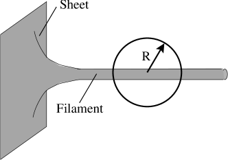
Figure 1: This shows an interconnected sheet and filament. Also shown, a sphere of radius $R$ centered on a galaxy located in the filament.

Though the Minkowski functionals and the Shapefinders are very effective techniques to quantify the shapes of individual structural elements like sheets or filaments, it is very different when dealing with the Cosmic Web which is an interconnected network of filaments, sheets and clusters. For example consider a sheet connected to a filament as shown in Figure 1. The Minkowski functionals are global properties of the entire object ie. the area is the sum of the areas of the sheet and the filament etc., and the fact that object is actually a combination of two different elements would be lost. It is necessary to quantify the local shape at different points in the object in order to determine that it actually is a combination of a sheet and a filament. In this paper we consider the “Local Dimension” as a means to quantify the local shape of the galaxy distribution at different positions along the Cosmic Web.

2 Method of Analysis

We choose a particular galaxy as center and determine $N(R)$ the number of other galaxies within a sphere of comoving radius $R$. This is done varying $R$. In the situation where a power law

$$N(R)=AR^{D}$$ (1)

gives a good fit over the length-scales $R_{1}\leq R\leq R_{2}$, we identify $D$ as the Local Dimension in the neighbourhood of the center. The values $D=1,2$ and $3$ correspond to a filament, sheet and cluster respectively. It may be noted that the term “cluster” here denotes a three dimensional, volume filling structural element and is not to be confused with a “cluster of galaxies”. Values of $D$ other than $1,2$ and $3$ are more difficult to interpret. For example, a galaxy distribution that is more diffuse than a filament but does not fill a plane would give a fractional value (fractal) in the range $1\leq D\leq 2$. Referring to Figure 1, we expect $D=1$ and $D=2$ when the center is located in the filament and the sheet respectively. This is provided that the center is well away from the intersection of the filament and the sheet. When the intersection lies within $R_{1}\leq R\leq R_{2}$ from the center, there will be a change in the slope of $N(R)$ when it crosses the intersection. It is not possible to determine a local dimension at the centers where such a situation occurs.

We perform this analysis using every galaxy in the sample as a center. In general it will be possible to determine a Local Dimension for only a fraction of the galaxies. It is expected that with a suitable choice of the $R$ range ie. $R_{1}$ and $R_{2}$, it will be possible to determine the Local Dimension for a substantial number of the centers. The value of the Local Dimension at different positions will indicate the location of the filaments, sheets and clusters and reveal how these are woven into the Cosmic Web.

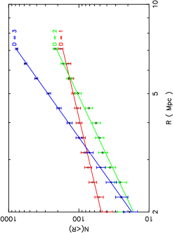
Figure 2: This shows $N(R)$ as a function of $R$ for three different centers from a particular realization. The centers have been chosen so as to demonstrate power law fits with $D\sim 1,2$ and $3$ corresponding to a filament, sheet and cluster respectively.

In this Letter we test this idea and demonstrate its utility by applying it to simulations. We have used a Particle-Mesh (PM) N-body code to simulate the $z=0$ dark matter distribution. The simulations have $256^{3}$ particles on a $256^{3}$ mesh with grid spacing $0.5\,{\rm Mpc}$. The simulations were carried out using a LCDM power spectrum with the parameters $(\Omega_{m0},\Omega_{\Lambda 0},h,n_{s},\sigma_{8})=(0.3,0.7,0.7,1,1)$. We have identified $210,000$ particles, randomly drawn from the simulation output, as galaxies. These have a mean interparticle separation of $\sim 2~{}{\rm Mpc}$, comparable to that in galaxy surveys. This simulated galaxy distribution was carried over to redshift space in the plane parallel approximation. The subsequent analysis to determine the Local Dimension was carried out using this simulated sample of $210,000$ galaxies. Since the resolution of the simulation is about $1\,{\rm Mpc}$, we can’t choose $R_{1}$ to be less than that. The value of $R_{2}$ is determined by the limited box size. We have chosen the value of $R_{1}$ and $R_{2}$ to be $2$ and $10\,{\rm Mpc}$ respectively. Increasing $R_{2}$ causes a considerable drop in the number of centers for which the Local Dimension is defined.

The analysis was carried out for $10$ different, independent realizations of the dark matter distribution. Figure 2 shows $N(R)$ for three different centers chosen from a particular realization. The $1-\sigma$ error at each data point is $\sqrt{N(r)}$ due to the Poisson fluctuation. For each center we have determined the power law $N(R)=AR^{D}$ that provides the best fit to the data. The power law fit is accepted if the chi-square per degree of freedom satisfies $\chi^{2}/\nu\leq 1.2$ and the value of $D$ is accepted as the Local Dimension corresponding to the particular center. The power law fit is rejected for larger values of $\chi^{2}/\nu$, and the Local Dimension is undetermined for the particular center. The criteria $\chi^{2}/\nu\leq 1.2$ is chosen as a compromise between a good power law fit and a reasonably large number of centers for which $D$ can been determined. The number of centers for which $D$ can been determined falls if a more stringent criteria is imposed on $\chi^{2}/\nu$.

3 Results and Conclusions

Figure 3: The galaxies within $10\,{\rm Mpc}$ of a center with $D\sim 1$ are shown as points. The galaxy distribution was converted to a set of 1s and 0s on a grid of spacing $1\,{\rm Mpc}$. Connected structures were identified using the Friend-of-Friend algorithm where adjacent 1s are identified as belonging to the same connected structure. Only the two largest structures have been shown, both pass very close to the center and they appear connected in the figure. The $D$ values have been painted on these structures with red, blue and green representing $D\sim 1,2$ and $3$ respectively. The $D$ value is undetermined for the parts of the structures shown in black.

The number of centers for which it is possible to determine a Local Dimension varies between $69,017$ to $73,481$ ie. less than $7\%$ variation across the $10$ different realizations. The $D$ values in the interval $1\pm 0.5$, $2\pm 0.5$ and $3\pm 0.5$ have respectively been binned as $D\sim 1,2$ and $3$. We have inspected the galaxy distribution in the vicinity of a few centers in order to visually identify the structures corresponding to the respective $D$ values. Figure 3 shows the galaxy distribution within $10\,{\rm Mpc}$ of a center which has Local Dimension $D\sim 1$. We expect this center to be located in a filament. We have used the Friend-of-Friend algorithm with linking length $\sqrt{3}\,{\rm Mpc}$ to identify connected patterns in the galaxy distribution. We note that all the galaxies in this region connect up into a single structure if the linking length is doubled to $2\times\sqrt{3}\,{\rm Mpc}$. Using $\sqrt{3}\,{\rm Mpc}$ yields several disconnected structures of which we show only the largest two. Both the structures pass close to the center, and appear connected in the figure. Of the two structures, one with two well separated tentacles appears below the center, whereas the other with two nearly connected tentacles appears above it. The filamentary nature of these structures is quite evident. Out of the total $79$ galaxies in these two structures, $D$ is undetermined for $58$. There are $8$ galaxies with $D\sim 1$, all located in a contiguous region near the center, and $6$ and $7$ galaxies with $D\sim 2$ and $3$ respectively spread out along the structure at locations quite different from the center. While it is relatively easy to visually identify the filament corresponding to the centers with $D\sim 1$, we have not been able to visually identify the sheets and clusters corresponding to the centers with $D\sim 2$ and $3$ shown in Figure 3. We note that a visual identification of the sheets and clusters corresponding to $D\sim 2$ and $3$ respectively has been possible in other fields where the largest structure is predominantly sheetlike or clusterlike. It is quite apparent that the largest structure in Figure 3 is predominantly filamentary.

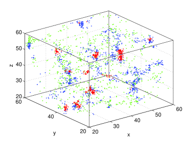
Figure 4: This shows the distribution of $D$ values in a box of size $[40\,{\rm Mpc}]^{3}$, red, blue and green denote $D\sim 1,2$ and $3$ respectively.

Figure 4 shows the distribution of $D$ values over a large region from one of the realizations. The distribution shows distinct patterns, there being regions with size ranging from a few ${\rm Mpc}$ to tens of ${\rm Mpc}$ where the $D$ value is constant. The centers with $D\sim 1$ appear to have a more dense and compact distribution compared to the centers with $D\sim 2$, whereas the centers with $D\sim 3$ appear to have a rather diffuse distribution.

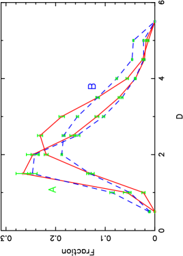
Figure 5: (A) The fraction of centers with a particular $D$ value, and (B) the volume fraction containing a particular $D$ value. The bins in $D$ have size $\pm 0.25$. The solid and dashed curves use $D$ values determined over length-scales $2-10\,{\rm Mpc}$ and $2-5\,{\rm Mpc}$ respectively.

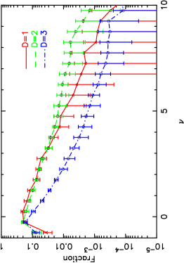
Figure 6: For each $D$ value we separately show the fraction of centers as a function of the density environment. The latter is quantified through $\nu=\delta/\sigma$ where $\delta$ is the density contrast and $\sigma^{2}$ its variance. This is evaluated on a grid of spacing $1\,{\rm Mpc}$ and the density field is smoothened with a Gaussian of width $5\,{\rm Mpc}$.

Figure 5 separately quantifies two different aspects of the distribution of $D$ values, (A.) the fraction of centers with a particular $D$ value, and (B.) the fraction of volume with a particular $D$ value. For this analysis the $D$ values were divided into bins of width $\pm 0.25$ and the centers for which a $D$ value could not be determined were discarded. We find that the fraction of centers and the volume fraction both have very robust statistics with a variation of $\sim 10\%$ or less across the $10$ different realizations. We first consider the distribution of the fraction of centers with different $D$ values. The bin at $D=1.5$ contains the maximum number of centers, and the two bins at $D=1.5$ and $2$ together contain more than $50\%$ of the centers. This indicates that the maximum number of centers for which $D$ can be determined lie in sheets and filaments. Assuming that this is representative of the entire matter distribution, we conclude that the bulk of the matter is contained in sheets and filaments, with the sheets dominating. We next consider the the fraction of volume occupied by a particular $D$ value. We have estimated this using a mesh with grid spacing $1\,{\rm Mpc}$. Each grid position was assigned the $D$ value of the centers within the corresponding grid cell. Cells that contain centers with different values of $D$ were discarded. It was possible to assign a $D$ value to $\sim 35,000$ grid cells. We find that the distribution peaks at $D=2.5$, the peak is rather broad and more than $50\%$ of the volume for which it was possible to assign a $D$ value is occupied by values in the range $2$ to $3$. Assuming that this result is valid for the entire volume, we conclude that the volume is predominantly filled with sheets and clusters. While the matter is mainly contained in sheets and filaments, the filaments do not occupy a very large fraction of the volume. This leads to a picture where the filaments have relatively higher matter densities as compared to clusters. To test this we separately consider the centers with $D$ values $1,2$ and $3$, and for each value we determine the fraction of centers as a function of the density environment. The density was calculated on a $1\,{\rm Mpc}$ grid after smoothing with a Gaussian filter of width $5\,{\rm Mpc}$. We find (Figure 6) that in comparison to the centers with $D\sim 1$ and $2$, the centers with $D\sim 3$ are more abundant in under-dense regions in preference to the over-dense regions. This is consistent with the picture where filaments and sheets located along the Cosmic Web contain the bulk of the matter and also most of the high density regions, whereas the centers with $D\sim 3$ are predominantly located in under-dense regions away from the Cosmic Web, namely the voids.

The results presented above are specific to the length-scale range $2-10\,{\rm Mpc}$. It is quite possible that the relative abundance of clusters, sheets and filaments would be quite different if the same analysis were carried out over a considerably different range of length-scales, say for example $0.1-1\,{\rm Mpc}$. Here we have repeated the entire analysis using a smaller range of length-scales $2-5\,{\rm Mpc}$ for which the results are also shown in Figure 5. We find that the results are qualitatively similar to those obtained using $2-10\,{\rm Mpc}$, indicating that our conclusions regarding the relative abundance of clusters, sheets and filaments are quite robust and are not very sensitive to small changes in the range over which $D$ is determined. This also indicates that the $D$ values determined using length-scales $2-10\,{\rm Mpc}$ are not severely biased by the presence of other structural elements with $5-10\,{\rm Mpc}$ of the one on which the center is located.

In conclusion we note that the Local Dimension provides a robust method to quantify the shapes and probe the distribution of the different, interconnected structural elements that make up the Cosmic Web. We plan to apply this to the SDSS and other galaxy surveys in future.

References

- Adelman-McCarthy et al. (2006) Adelman-McCarthy, J. K., et al. 2006, ApJS, 162, 38
- Basilakos, Plionis, & Rowan-Robinson (2001) Basilakos, S., Plionis, M., & Rowan-Robinson, M. 2001, MNRAS, 323, 47
- Bharadwaj et al. (2004) Bharadwaj S., Bhavsar S. P., & Sheth J. V., 2004, ApJ, 606, 25
- Bharadwaj et al. (2000) Bharadwaj S., Sahni V., Satyaprakash B. S.,Shandarin S. F., & Yess C., 2000, ApJ, 528, 21
- Doroshkevich et al. (2004) Doroshkevich, A., Tucker, D. L., Allam, S., & Way, M. J. 2004, A&A, 418, 7
- Einasto et al. (1980) Einasto, J., Joeveer, M., & Saar, E. 1980, MNRAS, 193, 353
- Geller & Huchra (1989) Geller, M.J. & Huchra, J.P.1989, Science, 246, 897
- Gott, Mellot & Dickinson (1986) Gott J. R., Mellot, A. L., & Dickinson, M. 1986, ApJ, 306, 341
- Joeveer et al. (1978) Joeveer, M., Einasto, J., & Tago, E. 1978, MNRAS, 185, 357
- Mecke et al. (1994) Mecke K. R., Buchert T. & Wagner H., 1994, A&A, 288, 697
- Müller et al. (2000) Müller, V., Arbabi-Bidgoli, S., Einasto, J., & Tucker, D. 2000, MNRAS, 318, 280
- Pandey & Bharadwaj (2005) Pandey, B. & Bharadwaj, S. 2005, MNRAS, 357, 1068
- Pandey & Bharadwaj (2008) Pandey, B. & Bharadwaj, S. 2008, MNRAS, In Press
- Pimbblet, Drinkwater & Hawkrigg (2004) Pimbblet, K. A., Drinkwater, M. J., & Hawkrigg, M. C. 2004, MNRAS, 354, L61
- Sahni et al. (1998) Sahni V., Satyaprakash B. S., & Shandarin S. F., 1998, ApJ, 495, L5
- Shandarin & Yess (1998) Shandarin, S. F. & Yess, C. 1998, ApJ, 505, 12
- Shandarin & Zeldovich (1983) Shandarin S. F., & Zeldovich I. B., 1983, Comments on Astrophysics, 10, 33
- Shectman et al. (1996) Shectman, S. A.,Landy, S. D., Oemler, A., Tucker, D. L., Lin, H., Kirshner, R. P., & Schechter, P. L. 1996, ApJ, 470, 172
- White (1979) White S. D. M., 1979 MNRAS, 186, 145
- Zel’dovich , Einasto & Shandarin (1982) Zel’dovich, I. B., Einasto, J., & Shandarin, S. F. 1982, Nature, 300, 407