M-brane singularity formation

Abstract

We derive self-similar string solutions in a graph representation, near the point of singularity formation, which can be shown to extend to point-like singularities on M-branes, as well as to the radially symmetric case.

I Introduction

For more than 40 years, Barbashov and Chernikov (1966, 1967, 1968) (see also Whitham (1974)), various ways of solving the non-linear equation

$$\ddot{z}(1+z^{\prime 2})-z^{\prime\prime}(1-\dot{z}^{2})=2\dot{z}z^{\prime}\dot{z}^{\prime}$$ (1)

are known. Recent work on higher dimensional time-like zero mean curvature hypersurfaces includes Christodoulou (2007); Milbredt (2008); Hoppe (2008); Bellettini et al. (2008) Here we show that (1) can develop singularities in finite time, starting from finite initial data. The structure of these singularities is described by the self-similar ansatz

$$z(t,x)=z_{0}-\hat{t}+\hat{t}^{\alpha}h\left(\frac{x}{\hat{t}^{\beta}}\right)+\dots$$ (2)

where $\hat{t}:=t_{0}-t\rightarrow 0$ (the dots are indicating lower order terms). Inserting (2) into (1) one finds the above ansatz to be consistent provided $\beta=(1+\alpha)/2>1$, and

$$h^{\prime\prime}\left(2\alpha h-\frac{(\alpha+1)^{2}}{4}\xi^{2}\right)=(\alpha-1)\left[h^{\prime 2}+\alpha h-\frac{3}{4}(\alpha+1)\xi h^{\prime}\right]\;,$$ (3)

for (2) to be an asymptotic solution of (1). For consistency with a finite outer solution of (1), the profile $h$ must satisfy

$$h(\xi)\propto A_{\pm}\xi^{\frac{2\alpha}{\alpha+1}}\quad\mbox{for}\quad\xi\rightarrow\pm\infty$$ (4)

(for a general discussion of matching self-similar solutions to the exterior see Eggers and Fontelos (2008)).

The ansatz (2) is formally consistent for a continuum of similarity exponents $\alpha\geq 1$ and for any solution of the similarity equation (3). However, by considering the regularity of solutions of (3) in the origin $\xi=0$ the similarity exponent must be one of the sequence

$$\alpha=\alpha_{n}=\frac{n+1}{n},\quad n\in\mathbb{N},$$ (5)

certainly if $h(0)=0=h^{\prime}(0)$, and presumably in general (i.e. all relevant solutions of (3)). Of this infinite sequence, we believe that only $\alpha=2$ is realized for generic initial data; indeed, in this case

$$\xi=\zeta+c\zeta^{3}/3,\quad h(\xi)=\zeta^{2}/2+c\zeta^{4}/4,$$ (6)

which we will deduce from a parametric string solution corresponding to (1).

The importance of the similarity solution (2) lies in the fact that it can be generalized to arbitrary dimensions, in particular to membranes. We find that the same type of singular solution is observed in any dimension, even having the same spatial structure (6).

II The similarity equation

A way of satisfying (3) is to demand

$$L^{2}:=h^{\prime 2}+2\alpha h-(\alpha+1)\xi h^{\prime}=0.$$ (7)

(differentiating e.g. $(1+\alpha)\xi=h^{\prime}+2\alpha h/h^{\prime}$ one can eliminate $h^{\prime\prime}$, reducing (3) to an identity, as long as $h^{\prime}\neq 1$).

The transformation

$$h(\xi)=\xi^{2}g(\xi)=\xi^{2}\left(\frac{(1+\alpha)^{2}}{8\alpha}-\frac{v^{2}}{2\alpha}\right)$$ (8)

yields

$$-\frac{d\xi}{\xi}=\frac{vdv}{v^{2}\pm\alpha v+(\alpha^{2}-1)/4}=\frac{1}{2}\left(\frac{\alpha+1}{v\mp\frac{\alpha+1}{2}}-\frac{\alpha-1}{v\mp\frac{\alpha-1}{2}}\right)dv,$$ (9)

i.e. (choosing the upper sign)

$$\frac{\left|v-(\alpha+1)/2\right|^{\alpha+1}}{\left|v-(\alpha-1)/2\right|^{\alpha-1}}=\frac{E}{\xi^{2}}.$$ (10)

This yields solutions $v\in[(\alpha-1)/2,(\alpha+1)/2)$,

$$v\approx\frac{\alpha-1}{2}+\left(\frac{\xi^{2}}{E}\right)^{\frac{1}{\alpha-1}}+\dots\quad\mbox{as}\quad\xi\rightarrow 0$$ (11)

$$v\approx\frac{\alpha+1}{2}-\left(\frac{\xi^{2}}{E}\right)^{\frac{1}{\alpha+1}}+\dots\quad\mbox{as}\quad\xi\rightarrow\pm\infty,$$

i.e.

$$h(\xi)\geq 0,h(0)=0,$$ (12)

$$h(\xi)\propto\xi^{2}/2\quad\mbox{as}\quad\xi\rightarrow 0$$

$$h(\xi)\propto\frac{1+\alpha}{2\alpha}\xi^{\frac{2\alpha}{1+\alpha}}\quad\mbox{as}\quad\xi\rightarrow\pm\infty.$$

Note that these solutions are consistent with the growth conditions (4).

To solve the second order equation (3) we note that $\tilde{h}(\xi):=c\;h(\xi/\sqrt{c})$ solves (3), if $h$ does, and that

$$\frac{h^{\prime}}{\xi}-\frac{2h}{\xi^{2}}=\frac{1}{\alpha}f\left(\sqrt{\frac{(\alpha+1)^{2}}{4}-2\alpha\frac{h(\xi)}{\xi^{2}}}\right)\quad\equiv\left(\frac{1}{\alpha}f(v)\right)$$ (13)

reduces (3) to

$$-\left(v^{2}-\frac{(\alpha+1)^{2}}{4}\right)\left(v^{2}-\frac{(\alpha-1)^{2}}{4}\right)=f\left(\alpha vf^{\prime}-(\alpha-1)f-(\alpha+2)v^{2}+(\alpha^{2}-1)(\alpha-2)/4\right),$$ (14)

and

$$\frac{d\xi}{\xi}=-\frac{vdv}{f(v)}=\frac{\alpha dg}{f}.$$ (15)

The growth condition (4) implies that $h$ grows less than quadratically at infinity. Thus we deduce from (13) that $f$ vanishes at $(\alpha+1)/2$. Furthermore, from a direct calculation using the growth exponent (4) we find the first derivative, yielding the initial conditions

$$f\left(\frac{\alpha+1}{2}\right)=0,\quad f^{\prime}\left(\frac{\alpha+1}{2}\right)=1.$$ (16)

Using (16), (14) yields a polynomial solution

$$f(v)=\left(v-\frac{(\alpha+1)}{2}\right)\left(v-\frac{(\alpha-1)}{2}\right)=v^{2}-\alpha v+\frac{\alpha^{2}-1}{4},$$ (17)

(i.e.) (10), which corresponds to the first order equation (7), but also an infinity of other solutions (a Taylor expansion around $v_{\infty}=(\alpha+1)/2$ shows that (14) leaves $f^{\prime\prime}((\alpha+1)/2)$ undetermined, when (16) holds). We note that (14) also has the solution $f_{-}(v)=f(-v)$, and for the special case $\alpha=2$ another pair of polynomial solutions,

$$\tilde{f}(v)=\left(v+3/2\right)\left(v-1/2\right)=v^{2}+v-3/4,$$ (18)

and $\tilde{f}_{-}(v)=\tilde{f}(-v)$. While the asymptotic behavior following from (18) is in disagreement with (4), integration methods similar to those used by Abel Abel (1881) perhaps permit a complete reduction of (14) to quadratures.

In any case, (14) can be simplified in various ways. For $\alpha=2$, e.g. it reduces to

$$yy^{\prime}=y-\frac{1}{4v^{5/2}}(v^{2}-9/4)(v^{2}-1/4)$$ (19)

via

$$f(v)=\sqrt{v}y(4v^{3/2}/3).$$ (20)

The solution (17), which is consistent with the growth condition (4), is equivalent to the solution (10) of (7) given before. If one investigates the behavior of the solution in the origin (either using (10) directly or by series expansion of (7)), one finds that only for $\alpha=\alpha_{n}$ (cf. (5)) a smooth solution is possible. Thus the first consistent solution is found for $n=1$ or $\alpha=2$. Higher order solutions $n=2,3,\dots$ are also possible in principle. They have the property that apart from $f^{\prime\prime}(0)$, the first non-vanishing derivative is $f^{(2n+2)}(0)$. However, we believe that they correspond to non-generic initial conditions, whose derivatives have corresponding properties of vanishing up to a certain order. To demonstrate this point, one would have to perform a stability analysis of the corresponding solution Eggers and Fontelos (2008). In the string picture discussed below this can be shown explicitly, as higher order solutions correspond to non-generic initial data.

III Higher dimensions

The solutions of (7), found to govern singularities of (1), also apply to higher dimensions. The reason is that the left hand side of (7) is the leading order term of

$${\cal L}^{2}=1-\dot{z}^{2}+z^{\prime 2}.$$ (21)

In other words, the asymptotic singular solutions discussed above have ${\cal L}^{2}=0+$ lower order. In fact, differentiating (21) with respect to $t$ and $x$ one easily shows that ${\cal L}^{2}=0$ provides solutions of (1). In higher dimensions, differentiating $1-z^{\alpha}z_{\alpha}=0$ gives $z^{\alpha}z_{\alpha\beta}=0$, and hence

$$(1-z_{\alpha}z^{\alpha})\square z+z^{\beta}z^{\alpha}z_{\alpha\beta}=0.$$ (22)

Thus solutions of ${\cal L}^{2}=0$ also solve the M-brane equation (22) in arbitrary dimensions.

For the special case of radially symmetric membranes:

$$\ddot{z}(1+z^{\prime 2})-z^{\prime\prime}(1-\dot{z}^{2})-2\dot{z}z^{\prime}\dot{z}^{\prime}=\frac{z^{\prime}}{r}\left(1-\dot{z}^{2}+z^{\prime 2}\right)\equiv\frac{z^{\prime}}{r}{\cal L}^{2}.$$ (23)

Insert the radial version of the ansatz (2),

$$z(t,r)=-\hat{t}+\hat{t}^{\alpha}h\left(\frac{r-r_{0}}{\hat{t}^{\beta}}\right)+\dots,$$ (24)

into (23). If $r_{0}\neq 0$, the entire right hand side of (23) is of lower order in $\hat{t}$, and the similarity equation (3) remains the same. Geometrically, this corresponds to the singularity forming along a circular ridge of radius $r_{0}$.

If on the other hand $r_{0}=0$, i.e. the singularity forms along the axis, the right hand side is of the same order, and the similarity equation becomes

$$h^{\prime\prime}\left(2\alpha h-\frac{(\alpha+1)^{2}}{4}\xi^{2}\right)+(1-\alpha)\left[h^{\prime 2}+\alpha h-\frac{3}{4}(\alpha+1)\xi h^{\prime}\right]=-\frac{h^{\prime}}{\xi}\left[h^{\prime 2}+2\alpha h-(\alpha+1)\xi h^{\prime}\right].$$ (25)

This equation can in principle have solutions different from (3). For solutions of (7), however, the expression in angular brackets in (25) vanishes, hence solutions of (7) also solve (25). Thus (24),(6) describe a point-like singularity on a membrane. These observations straightforwardly generalize to higher M-branes, $M>2$.

IV Parametric string solution

Let us now compare our findings with the solution of closed bosonic string motions given by equation (50) of Hoppe (1995). (note that the definitions of $f$ and $g$ are changed by $\pi/4$, and that the constant $\lambda$ is chosen to be 1):

$$\dot{{\bf x}}(t,\varphi)=\sin(f-g)\left(\begin{array}[]{c}-\sin(f+g)\\ \cos(f+g)\end{array}\right)$$ (26)

$${\bf x}^{\prime}(t,\varphi)=\cos(f-g)\left(\begin{array}[]{c}\cos(f+g)\\ \sin(f+g)\end{array}\right),$$ (27)

where $f=f(\varphi+t)$ and $g=g(\varphi-t)$. From (27) one finds the curvature

$$k(t,\varphi)=\frac{f^{\prime}+g^{\prime}}{\cos(f-g)}.$$ (28)

The hodograph transformation

$$(t,\varphi)\rightarrow t=x^{0},\quad x=x^{1}(t,\varphi),$$ (29)

$$x^{2}(t,\varphi)=z(t,x^{1}(t,\varphi)),$$

implying $\dot{z}=\dot{y}-\dot{x}y^{\prime}/x^{\prime}$, $z^{\prime}=y^{\prime}/x^{\prime}$, $(\partial\phi/\partial x^{0}=-\dot{x}/x^{\prime},(\partial\phi/\partial x^{1}=1/x^{\prime})$ permits to go between the parametric string picture (26)-(28) and the graph description (1). In particular,

$$1-\dot{z}^{2}+z^{\prime 2}=\left(\frac{\cos(f-g)}{\cos(f+g)}\right)^{2}$$ (30)

is manifestly non-negative in the parametric string-description, while for solutions of (1) one has to demand it explicitly - leading e.g. to the exclusion of solutions with $h^{\prime}(0)=0$, $h(0)<0$.

Let us give an explicit example of $\mathbb{M}_{2}\subset\mathbb{R}^{1,2}$ being at $t=0$ a regular graph, while for $t=1$ a curvature singularity has developed. Let $\mathbb{M}_{2}$ be described by ${\bf x}(\varphi,t)$, as defined by (26),(27), with $\varphi\in\mathbb{R}$, $t\geq 0$. Let

$$f(w)=\left\{\begin{array}[]{ll}\arctan w&\mbox{for}\quad w\geq\epsilon\\ \chi_{\epsilon}(w)\arctan w&\mbox{for}\quad 0\leq w\leq\epsilon<0\\ 0&\mbox{for}\quad w\leq 0\end{array}\right.,$$ (34)

where $\chi_{\epsilon}(w\geq\epsilon)=1$, $\chi_{\epsilon}(w\leq 0)=0$, and $\chi_{\epsilon}(0<w<0)$ such that $f^{\prime}(w)\geq 0$. We also assume that $g(w)=-f(-w)$. A simple calculation then shows that for $\varphi\in[-t+\epsilon,t-\epsilon]$ one obtains (${\bf x}_{0}(t=0,u=0)=0$)

$$x(\varphi,t)=-\varphi+\arctan(\varphi+t)+\arctan(\varphi-t)$$ (35)

$$y(\varphi,t)=\ln\sqrt{\left(1+(\varphi+t)^{2}\right)\left(1+(\varphi-t)^{2}\right)}$$

$$k(\varphi,t)=\frac{2}{\sqrt{\left(1+(\varphi+t)^{2}\right)\left(1+(\varphi-t)^{2}\right)}}\frac{\varphi^{2}+1+t^{2}}{\varphi^{2}+1-t^{2}}$$

Note that for $t>1$ this is no longer a graph.

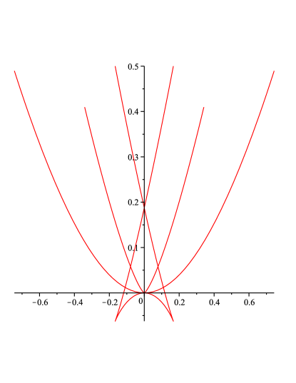
Figure 1: The formation of a swallowtail, as described by (40). Shown is a smooth minimum, ($\hat{t}>0$), a minimum with a 4/3 singularity ($\hat{t}=0$), and a swallowtail or double cusp ($\hat{t}<0$).

The example (34) underlies a general structure that can be uncovered by a local expansion of the functions $f$ and $g$ around the singularity. Namely, as seen from (28), the singularity occurs when $f-g$ is a multiple of $\pi/2$; for simplicity, we also assume that $g(w)=-f(-w)$ as before.

Then a local Taylor expansion yields

$$f(\zeta)=\pi/4+a(\zeta-\zeta_{0})-b(\zeta-\zeta_{0})^{2}+O(\zeta-\zeta_{0})^{3},$$ (36)

so together with the symmetry requirement we find

$$f-g=\pi/2+2a(t-\zeta_{0})-2b\varphi^{2}+(t-\zeta_{0})^{2},$$ (37)

where we neglected higher-order terms in the expansion, which will turn out to be irrelevant for the singularity formation.

From this expression it is clear that $\zeta_{0}$ has to be identified with the singular time $t_{0}$ and $a>0$ for the solution to be regular for $t<t_{0}$. Similarly, one must have $b>0$ (otherwise $f-g$ would be $\pi/2$ at an earlier time), and the singularity occurs at $\varphi=0$. Thus to leading order we have

$$f-g\approx\pi/2-2a\hat{t}-2b\varphi^{2},\quad f+g\approx 2a\varphi,$$ (38)

from which we get

$$x^{\prime}=2a\hat{t}+2b\varphi^{2},\quad y^{\prime}=4a^{2}\hat{t}\varphi+4ab\varphi^{3}.$$ (39)

Integrating this expression, using the integrability condition (27), gives

$$x=\hat{t}\varphi+c\varphi^{3}/3,\quad y=-\hat{t}+\hat{t}\varphi^{2}/2+c\varphi^{4}/4,$$ (40)

where we have used a rescaling of the parameter $\varphi$.

The curve described by (40) is shown in Fig. 1, but disregarding the spatial translation of $z$ by the term $-\hat{t}$. In catastrophe theory, this is known as the swallowtail Arnold (1984). For $\hat{t}>0$ the curve is smooth, while for $\hat{t}=0$ a rather mild singularity develops; at the origin, $y\propto x^{4/3}$. After the singularity ($\hat{t}<0$) the curve self-intersects. The solution (40) leads directly to the similarity form (2), if one notices that $\varphi$ is of order $\hat{t}^{1/2}$ for the terms in (40) to balance. Thus, using the notation of (2), and putting $\zeta=\varphi/\hat{t}^{1/2}$, one finds $\alpha=2,\beta=3/2$ for the exponents, and (6) for the similarity function. The crucial point is that although (6) came out of an expansion, all higher order terms are subdominant in the limit $\hat{t}\rightarrow 0$. Thus (6) is in fact an exact solution of (3) with $\alpha=2$. Moreover, it is even a solution of (7), and precisely of the form (10).

In the case of non-generic initial conditions other solutions are possible. For example, instead of (36)

$$f(\zeta)=\pi/4+a(\zeta-\zeta_{0})-b(\zeta-\zeta_{0})^{2n},$$ (41)

where $n\in\mathbb{N}$ but $n>1$. Only even powers $2n$ are allowed, otherwise the singularity occurs for all $\varphi$ at the same time, i.e. it is no longer point-like. If the leading order term is not linear but itself of higher order, the resulting similarity profile becomes singular at the origin, cf. 51. Repeating the above calculation along the same lines, we find

$$x^{\prime}=2a\hat{t}+2b\varphi^{2n},\quad y^{\prime}=4a^{2}\hat{t}\varphi+4ab\varphi^{2n+1},$$ (42)

which is equivalent to the symmetric shape function

$$\xi=\zeta+2d(n+1)\zeta^{2n+1}/(2n+1)$$ (43)

$$h=\zeta^{2}/2+d\zeta^{2n+2}.$$

The corresponding similarity exponent is $\alpha=\alpha_{n}$, as given by (5). We thus retrieve the exact same solutions identified by our previous analysis, based on a similarity description.

*

Appendix A Additional solutions of the similarity equation

It is possible to construct many more solutions to the similarity equation (7), which are all defined on the real line, but which we reject since they either contradict (4) or are not smooth. The simplest case is

$$h(\xi)=\frac{\xi^{2}}{2},$$ (44)

which is a solution for any $\alpha$, but evidently does not satisfy the matching condition (4).

Recall that for $\alpha=\alpha_{n}$, (10) furnishes smooth solutions on the real line. On the other hand, while for $\alpha=3$ the second derivative of the resulting solution is well-defined, the third derivative is discontinuous. Namely, for $E=4$ (e.g.) one finds that for $\xi>0$,

$$h(\xi)=-\frac{2}{3}\left(\xi+2(1+\xi)-2(1+\xi)^{3/2}\right)$$ (45)

$$h^{\prime}(\xi)=2\left(\sqrt{1+\xi}-1\right)>0$$

$$h^{\prime\prime}(\xi)=1/\sqrt{1+\xi},$$

so that

$$h^{\prime\prime\prime}(\xi)=\left\{\begin{array}[]{ll}-(1+\xi)^{-3/2}/2&\mbox{for}\quad\xi>0\\ (1+\xi)^{-3/2}/2&\mbox{for}\quad\xi<0.\\ \end{array}\right.$$ (48)

Other solutions whose scaling exponent is not from the set (5), but which have well-defined second derivatives, can be found from the parametric string solution as described in section IV. If the expansion of $f$ does not start with a linear term as in (36), but at higher order, e.g.

$$f(\zeta)=\pi/4+(\zeta-\zeta_{0})^{3}/2-b(\zeta-\zeta_{0})^{4},$$ (49)

one finds instead of (39)

$$x^{\prime}=3\hat{t}\varphi^{2}+2b\varphi^{4},\quad y^{\prime}=3\hat{t}\varphi^{5}+2b\varphi^{7}.$$ (50)

Integrating (50), the result once more conforms with (2), with a similarity exponent of $\alpha=4$, and the similarity function has the parametric form

$$\xi=\zeta^{3}+2b\zeta^{5}/5$$ (51)

$$h=\zeta^{6}/2+b\zeta^{8}/4.$$

It is confirmed easily that (51) solves (7) with $\alpha=4$, but the third derivative of $h(\xi)$ is singular at the origin.

References

Barbashov and Chernikov (1966)
B. M. Barbashov
and N. A.
Chernikov, Sov. Phys. JETP
23, 861 (1966).
Barbashov and Chernikov (1967)
B. M. Barbashov
and N. A.
Chernikov, Sov. Phys. JETP
24, 437 (1967).
Barbashov and Chernikov (1968)
B. M. Barbashov
and N. A.
Chernikov, Sov. Phys. JETP
27, 971 (1968).
Whitham (1974)
G. B. Whitham,
Linear and Nonlinear Waves (John
Wiley & Sons, 1974).
Christodoulou (2007)
D. Christodoulou,
The Formation of Shocks in 3-dimensional Fluids
(EMS Monographs in Mathematics, 2007).
Milbredt (2008)
O. Milbredt,
The Cauchy problem for membranes,
Ph.D. Thesis, FU Berlin (2008).
Hoppe (2008)
J. Hoppe,
Non-linear realization of Poincaré invariance in
the graph-representation of extremal hypersurfaces (2008),
URL http://arxiv:0806.0656.
Bellettini et al. (2008)
G. Bellettini,
M. Novaga, and
G. Orlandi,
Time-like Lorentzian minimal submanifolds as singular
limits of nonlinear wave equations (2008).
Eggers and Fontelos (2008)
J. Eggers and
M. A. Fontelos,
The role of self-similarity in singularities of partial
differential equations (2008),
URL http://arXiv:0812.1339.
Abel (1881)
N. H. Abel,
Oeuvres II (Imprimerie de
Grøndahl & Søn, Christiania, 1881).
Hoppe (1995)
J. Hoppe,
Conservation laws and formation of singularities in
relativistic theories of extended objects (1995),
URL http://arxiv:hep-th/9503069.
Arnold (1984)
V. I. Arnold,
Catastrophe Theory (Springer,
1984).