Efficiency of structured adiabatic quantum computation

Abstract

We show enough evidence that a structured version of Adiabatic Quantum Computation (AQC) is efficient for most satisfiability problems. More precisely, when the success probability is fixed beforehand, the computational resources grow subexponentially in the number of qubits. Our study focuses on random satisfiability and exact cover problems, developing a multi-step algorithm that solves clauses one by one. Relating the computational cost to classical properties of the problem, we collect significant statistics with up to $N=140$ qubits, around the phase transitions, which is where the hardest problems appear.

While the general framework of Quantum Computation is to a large extent justified by the progressive miniaturization of integrated circuits, there is still a major open problem in the field which is the finding of new quantum algorithms. This task is rather difficult due to both the lack of a fully quantum programming model and the general requirement that any quantum algorithm should outperform its classical counterparts –a perhaps too ambitious expectation which imposes both proofs of the classical and quantum complexities.

The Adiabatic Quantum Computation paradigm Farhi et al. (2001) is a very appealing framework for the development of new algorithms. While equivalent to the circuit model Aharonov et al. (2004), this paradigm aims at adiabatically preparing the ground state of a quantum Hamiltonian, a state which encodes the solution to a problem we want to solve. The resource that measures the computational cost in AQC is the time required to prepare the state and the adiabatic theorem Messiah (1999) provides a criterion to bound this time, either numerically or analytically. In addition to this, the adiabatic formulation is particurlarly well suited for constraint solving problems. The constraints may be encoded as energy penalties in a Hamiltonian, so that any solution of the whole problem must be a ground state of the final Hamiltonian.

The traditional interest on AQC is precisely rooted on its relation to constraint solving and in particular to logical satisfiability (SAT) problems. From a practical point of view, many real-world problems, including automated hardward design and verification, can be suitably represented in SAT form. Furthermore, the subset of 3SAT problems were also the first problems shown to be NP-complete Cook (1971); Levin (1973). This implies that if we had an algorithm to efficiently solve 3SAT, we could also solve all problems in the much larger NP family . However, to date, the extensive literature about classical SAT algorithms suggests that these problems are exponentially hard to solve Skjernaa (2004), even in the average and typical cases Coarfa et al. (2003).

Regarding the utility of quantum computation in solving SAT problems, there is not yet a clear cut answer. Despite the promising results of the very first AQC simulations Farhi et al. (2001), nowadays AQC is expected to be expontentially costly for the worst-case instances of NP-complete SAT problems van Dam et al. (2001); Ambainis (2004); Aaronson (2006); Žnidarič (2005), when no use of the structure of the problem is made. One may argue that the worst-case complexity is less relevant than the average-case cost Levin (1986), and there are evidences for average exponential speedups in the quantum query problem Ambainis and de Wolf (2001). Many works have adopted this point of view and studied the running times of average or typical adiabatic computations Farhi et al. (2001); Hogg (2003); Latorre and Orús (2004); Bañuls et al. (2006); Schutzhold and Schaller (2006); Young et al. (2008). Here the results are still mixed, ranging from polynomial Young et al. (2008) to subexponential Farhi et al. (2001); Bañuls et al. (2006) and to exponential Hogg (2003) growth. These discrepancies can be attributed to the difficulty of simulating a quantum algorithm, which limits the analysis to small instances and statistical samples.

In this work we want to rule out not only the worst-case restriction, but also the use of unstructured algorithms. We will introduce a new composite algorithm for SAT that alternates diabatic and adiabatic stages. We will then relate the running times of the algorithm to classical properties of the SAT instances. Using this connection, we exactly characterize the performance of the algorithm for very large problems, with a much larger sampling space than any previous study —up to $N=140$ bits with $2\times 10^{6}$ instances—. With this data we will answer a question of great practical relevance: given a desired success probability, what is the scaling of the resources required to solve that fraction of randomly picked, but classically hard problems. The result will be that the resources grow subexponentially, even in regimes in which the classical algorithms would be exponentially costly Coarfa et al. (2003).

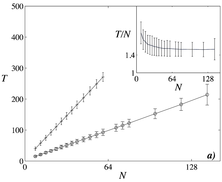
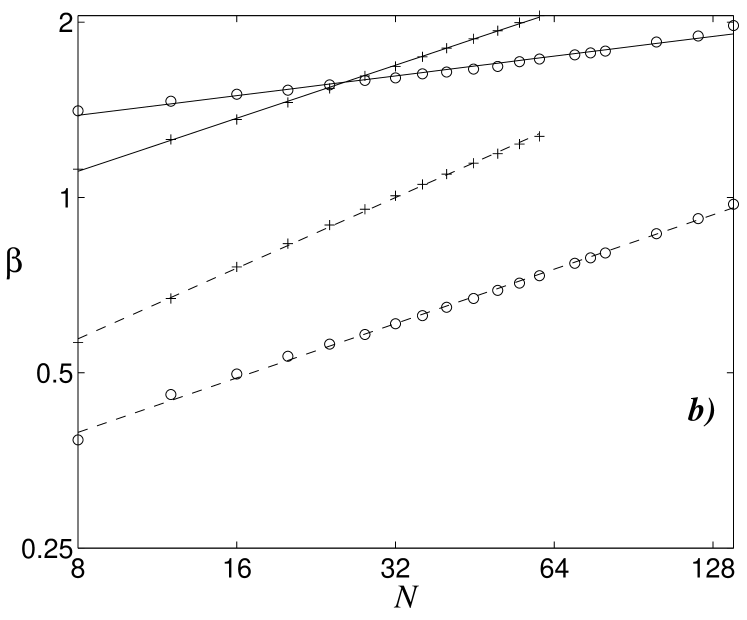
Figure 1: Efficiency of the quantum algorithm. In (a) we plot the total running time vs. the number of qubits. We have used Eq. (1) with $\Omega=1.$ We plot average results for X3SAT (circles) and 3SAT (crosses) together with standard deviations. The inset shows the deviation from a linear law for X3SAT. Figure (b) is a log-log plot of the average value (solid) and variance (dashed) of the value $\beta,$ which is the logarithm of the maximum time required by one of the adiabatic intervals. The lines are fits to power laws, $\beta,\Delta\beta\sim aN^{b}.$ Each point in the plots involves $2\times 10^{6}$ random instances.

This work focuses on the solution of SAT problems. An instance of this family is defined by a set of $M$ logical constraints or clauses on a finite set of $N$ Boolean variables $(s_{1},s_{2}\ldots s_{N}).$ In the particular case of $p$-SAT, each clause is a Boolean function depending only on $p$ variables $f_{k}(s_{k_{1}},s_{k_{2}},\ldots s_{k_{p}}):\{0,1\}^{\otimes p}\to\{0,1\}.$ The problem is to determine whether there exists an assignment of the $N$ variables satisfying all $M$ clauses, a task for which there exist both heuristic and probabilistic classical algorithms.

Our quantum algorithm for SAT is a hybrid that alternates non-adiabatic evolution with adiabatic steps, in a way that goes beyond structured AQC Roland and Cerf (2003). The key ingredients are to initially sort the set of logical clauses, and to have each adiabatic step solving a single clause. Let us call $S_{m}$ the set of assignments which are compatible with the $m$ first logical clauses. As shown below, during the $m$-th time interval of adiabatic evolution $(t_{m-1},t_{m}),$ the quantum register will evolve from a linear superposition of all states in $S_{m-1}$ to a linear superposition of those in $S_{m}.$ For this step of the computation to succeed we require a run time

$$t_{m}-t_{m-1}=\Omega\times{d_{m-1}}/{d_{m}},$$ (1)

where $d_{m}=|S_{m}|$ is the size of the set $S_{m}$ and $\Omega$ is some big multiplicative constant specified by the adiabatic theorem Messiah (1999). This relates the resource of the adiabatic algorithm —time— to a classical property —the structure of solution spaces—, and it will be the main tool in our analysis of the efficiency. Note that if we add all clauses in the same adiabatic interval, the adiabatic time becomes exponentially large $T_{\mathrm{search}}\sim\Omega d_{0}/{d_{M}}\sim 2^{N},$ consistently with search algorithms for unstructured problems Roland and Cerf (2002). Let us now present the algorithm and derive Eq. (1).

The algorithm.

In AQC, the solution of a computational problem is encoded in a state $\psi_{g}$ which is the ground state of a problem Hamiltonian, $H_{P}$. To prepare $\psi_{g},$ the Hamiltonian of the quantum register is slowly modulated from an initial operator $H(0)$ with an easily prepared ground state $\psi(0)$, up to our final operator $H(T)=H_{P}.$ The adiabatic theorem states that if the evolution is slow enough, the quantum register will end up in the desired state, $\psi(T)=\psi_{g}.$ The condition “slow enough” evolution means that the changes in the Hamiltonian happen in a long time scale $T\gg 1/(\Delta E)^{2},$ larger than the minimal gap $\Delta E$ between the ground state manifold and the excited states of $H(t)$.

In our algorithm the initial state is a linear combination of all states in the computational basis $\left|{\psi(0)}\right\rangle\propto\sum_{\mathbf{s}}\left|{\mathbf{s}}\right\rangle=\left(\left|{0}\right\rangle+\left|{1}\right\rangle\right)^{\otimes N}.$ This product state is evolved with a Hamiltonian that is piecewise continuous. Within the $m$-th interval, $t\in\left(t_{m-1},t_{m}\right),$ we write

$$H(t)=H_{C}^{(m)}+[1-\lambda_{m}(t)]H_{B}^{(m)}+\lambda_{m}(t)H_{P}^{(m)},$$ (2)

with adiabatic parameter $\lambda_{m}(t)=(t-t_{m-1})/(t_{m}-t_{m-1})$. The three operators are

$$H_{P}^{(m)}\left|{\mathbf{s}}\right\rangle = \left[1-f_{m}(s_{m_{1}},s_{m_{2}},s_{m_{3}})\right]\left|{\mathbf{s}}\right\rangle,$$ (3)

$$H_{B}^{(m)}\left|{\mathbf{s}}\right\rangle = -\frac{1}{2^{N/2}}\sum_{\mathbf{s}^{\prime}}\left|{\mathbf{s}^{\prime}}\right\rangle,\;\mathrm{and}$$ (4)

$$H_{C}^{(m)} = \Gamma\sum_{k=1}^{m-1}H_{P}^{(k)}.$$ (5)

Respectively, a term that penalizes invalid configurations for the $m$-th clause, a component that mixes all possible configurations and an operator that penalizes any violation of the $m-1$ clauses we have solved so far. We expect that, if the adiabatic steps succeed and the non-adiabatic steps do not introduce significant errors, after each time $t_{m}$ the register will be in a linear combination of all assignments which are compatible with the $m$ first logical clauses, $\psi(t_{m})\simeq\left|{\Xi_{m}}\right\rangle\propto\sum_{s\in S_{m}}\left|{s}\right\rangle.$

Non-adiabatic errors.

In between adiabatic intervals the Hamiltonian changes non-adiabatically from $H(t_{m}^{-})$ to $H(t_{m}^{+}).$ This implies strengthening the last clause by a factor $\Gamma$ and switching on the term $H_{B}^{(m)}.$ Without affecting the execution time, this process introduces a controllable error on the state, which amounts to the difference between the ground states of $H(t)$, that is $\psi_{g}(t),$ immediately before $t_{m}$ and after it. Applying the results in Ref. Aharonov et al. (2004) we obtain $\left\langle\psi_{g}(t_{m}^{+})|\psi_{g}(t^{-}_{m})\right\rangle\leq 1-\frac{1}{\Gamma-1}.$ Since the difference is ${\cal O}(1/\Gamma),$ the $M$ adiabatic steps will amount to an overall error $M/\Gamma,$ which can be decreased with resources that are polynomial in $M.$

Cost of the algorithm.

Given the previous assumption that the constraints term is dominant, $\Gamma\gg 1,$ we may diagonalize the model Hamiltonian (2) approximately, and thus compute the minimum energy gap during each adiabatic step. We separate the Hilbert space into two parts, ${\cal H}={\cal H}_{m-1}\oplus{\cal H}^{\perp}_{m-1},$ the space of solutions which are compatible with the previous $m-1$ clauses, ${\cal H}_{m-1}=\mathrm{lin}\{\left|{\bf s}\right\rangle,{\bf s}\in S_{m-1}\},$ and its orthogonal complement. During each interval $(t_{m-1},t_{m}),$ the low energy spectrum of $H(t)$ is approximately given Aharonov et al. (2004) by that of its projection onto ${\cal H}_{m-1},$ an operator that we call $H_{m-1}(t).$ In the two dimensional space spanned by the vector $\Xi_{m}$ and its complement $\left|{\Xi^{\perp}_{m}}\right\rangle\propto\sum_{\mathbf{s}\in{\bar{S}}_{m}\cap S_{m-1}}\left|{\mathbf{s}}\right\rangle,$ we may write $H_{m-1}=(\lambda_{n}-\frac{1}{2})\mathbb{I}+\frac{1}{2}(\lambda-1)\sin(2\alpha_{n})\sigma^{x}+\frac{1}{2}\left[(\lambda_{n}-1)\cos(2\alpha_{n})-\lambda\right]\sigma^{z},$ expressed using the Pauli matrices and $\cos(\alpha_{n})=\sqrt{d_{n}/d_{n-1}}=\left\langle\Xi_{m}|\Xi_{m-1}\right\rangle$. This matrix has a minimal separation or energy gap at $\lambda_{n}=1/2,$ given by $\Delta E_{m}=\cos(\alpha_{m})=\sqrt{d_{m}/d_{m-1}}.$ This provides a first estimate for the running time of the adiabatic step, $t_{m}-t_{m-1}\gg 1/(\Delta E_{m})^{2}$ or Eq. (1). But for this reasoning to be complete, we must also consider the influence of states with energy $\gg\Gamma.$ Following Ref. Aharonov et al. (2004) the high energy states produce corrections in the energy gap and the ground state wavefunctions which are small, ${\cal O}(1/\Gamma)$. Therefore, by imposing a penalty $\Gamma\simeq\kappa\sqrt{d_{n-1}/d_{n}}$ at each step, with a constant $\kappa\gg 1$, or using a global $\Gamma$ larger than all the individual factors, we can ensure that Eq. (1) still holds. Finally, since multiplicative factors in the Hamiltonian affect the total running time, one should actually consider an adimensional running time Aharonov et al. (2004) such as $\tilde{T}=T\max_{s}\|H(s)\|\sim T\times\Gamma,$ but with the previous choices, both $T$ and $\tilde{T}$ scale similarly.

Performance.

For our benchmarks we have chosen two sets of problems: Exact Cover and 3SAT in conjunctive normal form (CNF). The first family, also known as X3SAT (or one-in-three SAT), has clauses that require exactly one bit to be set: $f_{k}(s_{k_{1}},s_{k_{2}},s_{k_{3}})=1$ iff $s_{k_{1}}+s_{k_{2}}+s_{k_{3}}=1.$ These problems have been extensively used to test the efficiency of unstructured adiabatic quantum computationFarhi et al. (2001); Latorre and Orús (2004); Childs et al. (2001); Bañuls et al. (2006). However, it is known that even though they form an NP-complete set, Exact Cover problems tend to be easier than general 3SAT ones. Hence, we have also studied this more general set of problems, casting them in a convenient form: $f_{k}(s_{k_{1}},s_{k_{2}},s_{k_{3}})=0$ iff $s_{k_{1}}=a_{k},\,s_{k_{2}}=b_{k},\,s_{k_{3}}=c_{k},$ where each function forbids a precise combination $(a_{k},b_{k},c_{k})$ of the bits involved.

Our statistical study is based on a random sampling of 3SAT and X3SAT problems, generated with a bias towards hard instances. This is done by fixing the ratio of clauses to bits, $\alpha=M/N,$ close to the phase transition from trivially satisfiable problems to problems with no solution. It is known that the density of hard problems is highest around these narrow regions Mitchell et al. (1992); Achlioptas et al. (2000, 2005); Kalapala and Moore ; Raymond et al. (2007), $\alpha_{SAT}\in(4,4.24)$ and $\alpha_{X3SAT}\in(0.54,0.64),$ while the outer regions can be easily solved using specialized solvers. For each instance we generate $M$ clauses, each one acting on three different random bits. In the case of 3SAT we also generate the random bit sequences to be rejected, $(a_{k},b_{k},c_{k})$. Our pseudo-random number generator is a Mersenne-Twister Matsumoto and Nishimura (1998) which has a period $\sim 2^{19937}$ and good equidistribution properties.

We have applied our algorithm to a sufficiently large selection of randomly generated 3SAT and Exact Cover instances. For each random instance of 3SAT or X3SAT the clauses are sorted according to the indices of the bits that are involved. We loop over the sorted clauses, iteratively creating the space of valid assignments, which is decomposed into configurations of the $n_{a}(m)$ active and $N-n_{a}(m)$ inactive bits, $S_{m}=A_{m}\otimes I_{m}.$ Since $d_{m}=|A_{m}|2^{N-n_{a}(m)}$, only $A_{m}$ needs to be stored and computed. The set $A_{m}$ itself is created from $A_{m-1}$ using a parallelized algorithm which involves 128 processors and a total of 256Gb of memory for the largest problems. Note that sorting the clauses is an essential ingredient to make both $n_{a}(m)$ and $|A_{m}|$ grow slowly.

The optimal total running time $t_{M}$ is computed as the sum over all clauses of the terms in Eq. (1). As shown in Fig. 1a it has an average behavior which is close to linear in the number of bits. However, preparing an experiment that runs in this optimal time requires some knowledge about the solution spaces, as some intervals require more time than others. A more realistic goal is choosing a running time that ensures a high probability of success for arbitrary instances. For this we introduce a new variable

$$\beta=\max_{m}\log_{2}(d_{m-1}/d_{m}),$$ (6)

with which we can uniformly bound the total running time of a given problem as

$$t_{M}\leq\Omega M\times 2^{\beta}.$$ (7)

We have computed the value $\beta$ for every instance in the samples. By studying the statistics of this quantity over different problems we infer an optimal value, $\beta_{opt}(\sigma,N,M),$ such that running the quantum computer for a time $T_{opt}=\Omega M\exp(\beta_{opt})$ ensures the correct solution of a large fraction $\sigma$ (say $\sigma=99.99\%$) of all $N$-bit hard instances. The scaling of $\beta_{opt}$ with respect to the problem size and success probability is a more meaningful characterization of the algorithm than the scaling of the worst case times.

The first results are shown in Fig. 1b, where we plot the average value of $\beta$ and its variance, and fit them to curves of the form $\beta_{X3SAT}=1.14N^{0.162},$ $\Delta\beta_{X3SAT}=0.1N^{0.447},$ and $\beta_{3SAT}=0.468N^{0.438},$ $\Delta\beta_{3SAT}=0.133N^{0.581}.$ Based on this, the running time without previous knowledge of the problem could be

$$T_{opt}\sim\Omega\times N\times 2^{\beta+6\Delta\beta}\sim N2^{cN^{r}},$$ (8)

where exponent $6\Delta\beta$ guarantees a very small probability of failure. This suggests an overall behavior that follows a sub-exponential law with $r<0.5$ for X3SAT and $r<0.6$ for 3SAT.

By studying the actual probability distribution of $\beta$ we can confirm the sub-exponential behavior, obtain a better choice of the running time and actually estimate the failure probability. Since $\beta$ cannot be larger than the number of bits, these distributions have all finite support. Nevertheless, as shown in Fig. 2, their tails can be accurately bounded by an exponential law $\exp(-\beta/\xi).$ According to this law, the failure probability of a particular setup which uses a running time $T_{opt}=\Omega M\exp(\beta_{opt})$ is bounded by

$$P_{\rm fail}=\int_{\beta_{opt}}^{\infty}P(\beta)d\beta\sim\exp(-\beta_{opt}/\xi).$$ (9)

Our numerical analysis reveals that $\xi$ grows algebraically with the number of bits. Therefore, a fixed success probability can be achieved with subexponential resources.

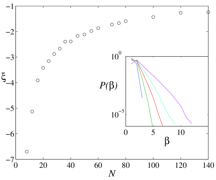
Figure 2: Probability distribution of algorithm running times. The inset shows the probability distributions, $P(\beta;N),$ of the logarithm of the interval that takes the most time in our algorithm (6), for $N=8,16,32,60$ and $140$ bits (left to right). These distributions are subject to an exponential fit $P(\beta;N)\sim\exp(-\beta/\xi),$ which gives the parameter $\xi(N)$ shown in the plot. This value grows subexponentially in the number of qubits and is a realistic measure of the algorithm efficiency.

Summing up, in this work we have presented a hybrid quantum algorithm which has the advantage that its efficiency can be computed at a relatively low cost. We have shown that it is possible to establish a running time such that the algorithm solves a large fraction of randomly picked but still classically hard problems. This time is found to scale subexponentially in the size of the problem, which is to be compared with the average exponential behavior of classical algorithms Coarfa et al. (2003). While the long range interactions make this algorithm suboptimal for implementation, our work opens the path to the development and analysis of other structured algorithms.

JJGR acknowledges support from Spanish projects FIS2006-04885 and CAM-UCM/910758. The computations for this work were performed at the Barcelona Supercomputing Center of Spain (BSC-CNS).

References

- Farhi et al. (2001) E. Farhi, J. Goldstone, S. Gutmann, J. Lapan, A. Lundgren, and D. Preda, Science 292, 472 (2001).
- Aharonov et al. (2004) D. Aharonov, W. van Dam, J. Kempe, Z. Landau, S. Lloyd, and O. Regev, Foundations of Computer Science, Annual IEEE Symposium on 0, 42 (2004).
- Messiah (1999) A. Messiah, Quantum Mechanics (Dover Publications, 1999), chap. xvii.
- Cook (1971) S. A. Cook, in STOC ’71: Proceedings of the third annual ACM symposium on Theory of computing (ACM, New York, NY, USA, 1971), pp. 151–158.
- Levin (1973) L. A. Levin, Problems of information transmission 9, 265 (1973).
- Skjernaa (2004) B. Skjernaa, Ph.D. thesis, University of Aarhus (2004).
- Coarfa et al. (2003) C. Coarfa, D. D. Demopoulos, A. S. M. Aguirre, D. Subramanian, and M. Y. Vardi, Constraints 8, 243 (2003).
- van Dam et al. (2001) W. van Dam, M. Mosca, and U. Vazirani, Foundations of Computer Science, 2001. Proceedings. 42nd IEEE Symposium on pp. 279–287 (2001).
- Ambainis (2004) A. Ambainis, SIGACT News 35, 22 (2004).
- Aaronson (2006) S. Aaronson, SIAM Journal on Computing 35, 804 (2006).
- Žnidarič (2005) M. Žnidarič, Phys. Rev. A 71, 062305 (2005).
- Levin (1986) L. A. Levin, SIAM Journ. Comp. 15, 285 (1986).
- Ambainis and de Wolf (2001) A. Ambainis and R. de Wolf, J. Phys. A: Math. Gen. 34, 6741 (2001).
- Hogg (2003) T. Hogg, Phys. Rev. A 67, 022314 (2003).
- Latorre and Orús (2004) J. I. Latorre and R. Orús, Phys. Rev. A 69, 062302 (2004).
- Bañuls et al. (2006) M. C. Bañuls, R. Orús, J. I. Latorre, A. Pérez, and P. Ruiz-Femenía, Phys. Rev. A 73, 022344 (2006).
- Schutzhold and Schaller (2006) R. Schutzhold and G. Schaller, Phys. Rev. A 74 (2006).
- Young et al. (2008) A. P. Young, S. Knysh, and V. N. Smelyanskiy, Phys. Rev. Lett. 101, 170503 (2008), arXiv:0803.3971.
- Roland and Cerf (2003) J. Roland and N. J. Cerf, Phys. Rev. A 68, 062312 (2003).
- Roland and Cerf (2002) J. Roland and N. J. Cerf, Phys. Rev. A 65, 042308 (2002).
- Childs et al. (2001) A. M. Childs, E. Farhi, and J. Preskill, Phys. Rev. A 65, 012322 (2001).
- Mitchell et al. (1992) D. Mitchell, B. Selman, and H. Levesque, in Proceedings of the Tenth National Conference on Artificial Intelligence (AAAI-92), San Jose, CA (1992), pp. 459–465.
- Achlioptas et al. (2000) D. Achlioptas, C. Gomes, H. Kautz, and B. Selman, in In AAAI/IAAI (AAAI Press, 2000), pp. 256–261.
- Achlioptas et al. (2005) D. Achlioptas, A. Naor, and Y. Peres, Nature 435, 759 (2005).
- (25) V. Kalapala and C. Moore, arXiv:cs/0508037.
- Raymond et al. (2007) J. Raymond, A. Sportiello, and L. Zdeborova, Phys. Rev. E 76, 011101 (2007).
- Matsumoto and Nishimura (1998) M. Matsumoto and T. Nishimura, ACM Trans. Model. Comput. Simul. 8, 3 (1998).