Local Star formation triggered by SN shocks in magnetized diffuse neutral clouds

Abstract

In this work, considering the impact of a supernova remnant (SNR) with a neutral magnetized cloud we derived analytically a set of conditions that are favorable for driving gravitational instability in the cloud and thus star formation. Using these conditions, we have built diagrams of the SNR radius, $R_{SNR}$, versus the initial cloud density, $n_{c}$, that constrain a domain in the parameter space where star formation is allowed. This work is an extension to previous study performed without considering magnetic fields (Melioli et al. 2006). The diagrams are also tested with fully 3-D MHD radiative cooling simulations involving a SNR and a self-gravitating cloud and we find that the numerical analysis is consistent with the results predicted by the diagrams. While the inclusion of a homogeneous magnetic field approximately perpendicular to the impact velocity of the SNR with an intensity $\sim 1\;\mu$G within the cloud results only a small shrinking of the star formation zone in the diagram relative to that without magnetic field, a larger magnetic field ($\sim 10\;\mu$G) causes a significant shrinking, as expected. Though derived from simple analytical considerations these diagrams provide a useful tool for identifying sites where star formation could be triggered by the impact of a SN blast wave. Applications of them to a few regions of our own galaxy (e.g., the large CO shell in the direction of Cassiopeia, and the Edge Cloud 2 in the direction of the Scorpious constellation) have revealed that star formation in those sites could have been triggered by shock waves from SNRs for specific values of the initial neutral cloud density and the SNR radius. Finally, we have evaluated the effective star formation efficiency for this sort of interaction and found that it is generally smaller than the observed values in our own Galaxy (sfe $\sim$ 0.01$-$0.3). This result is consistent with previous work in the literature and also suggests that the mechanism presently investigated, though very powerful to drive structure formation, supersonic turbulence and eventually, local star formation, does not seem to be sufficient to drive $global$ star formation in normal star forming galaxies, not even when the magnetic field in the neutral clouds is neglected.

1 Introdution

Essentially all present day star formation takes place in molecular clouds (MCs; e.g. Blitz 1993; Williams, Blitz & McKee 2000). It is likely that the MCs are relatively transient, dynamically evolving structures produced by compressive motions in the diffuse HI medium of either gravitational or turbulent origin, or some combination of both (e.g., Hartmann et al. 2001; Ballestero-Paredes et al. 2007). In fact, observations of supersonic line-widths in the MCs support the presence of supersonic turbulence in these clouds with a wealth of structures on all length-scales (Larson 1981; Blitz & Williams 1999; Elmegreen & Scalo 2004; Lazarian & Esquivel 2003). Recent numerical simulations in periodic boxes have shed some light on the role of the turbulence in the evolution of the MCs and the star formation within them. They suggest that the $continuous$ injection of supersonic motions, maintained by internal or external driving mechanisms (see below), can support a cloud $globally$ against gravitational collapse so that the net effect of turbulence seems to inhibit collapse and this would explain the observed low overall star formation efficiencies in the Galaxy (Klessen et al. 2000; Mac Low & Klessen 2004; Vazquez-Semandeni et al. 2005). On the other hand, the supersonic turbulence is also able to produce density enhancements in the gas that may allow $local$ collapse into stars in both nonmagnetized (Klessen et al. 2000; Elmegreen & Scalo 2004) and magnetized media (Heitsch et al. 2001; Nakamura & Li 2005).

What are the possible sources of this turbulence in the MCs? Suggested candidates for an internal driving mechanism of turbulence include feedback from both low-mass and massive stars. These later, in particular, are major structuring agents in the ISM in general (McCray & Snow 1979), initially through the production of powerful winds and intense ionizing radiation and, at the end of their lives through the explosions as supernovae (SNe). It is worth noting however, that MCs with and without star formation have similar kinematic properties (Williams, Blitz & McKee 2000). External candidates include galactic spiral shocks (Roberts 1969; Bonnell et al. 2006) and again SNe shocks (Wada & Norman 2001; Elmegreen & Scalo 2004). These processes seem to have sufficient energy to explain the kinematics of the ISM and can generate the observed velocity dispersion-sizescale relation (Kornreich & Scalo 2000). Other mechanisms, such as magnetorotational instabilities, and even the expansion of HII regions and fluctuations in the ultraviolet (UV) field apparently inject energy into the ambient medium at a rate which is about an order of magnitude lower than the energy that is required to explain the random motions of the ISM at several scales, nonetheless the relative importance of all these injection mechanisms upon star formation is still a matter of debate (see, e.g., Joung & Mac Low 2006; Ballesteros-Paredes et al. 2007; Mac Low 2008 for reviews).

In this work, we focus on one of these driving mechanisms $-$ supernova explosions produce large blast waves that strike the interstellar clouds, compressing and sometimes destroying them, but the compression by the shock may also trigger local star formation (Elmegreen & Lada 1977; see also Nakamura & Li 2005 and references therein). There has been extensive analytical and numerical work exploring the role of the SNe in generating supersonic turbulence and multi-phase structures in the ISM (e.g., Cox & Smith 1974; McKee & Cowie 1975; McKee & Ostriker 1977; Kornreich & Scalo 2000; Mac Low & Klessen 2004; Vazquez-Semadeni et al. 2000; de Avillez & Breitschwerdt 2005) and even at the galactic scale, in the generation of large-scale outflows like galactic fountains and winds (e.g., de Gouveia Dal Pino & Medina-Tanco 1999; de Avillez 2000; Heckman et al. 2001; de Avillez & Berry 2001; Melioli et al. 2008a, 2008b). The collective effect of the SNe is likely to be the dominant contributor to the observed supersonic turbulence in the Galaxy (Norman & Ferrara 1996; Mac Low & Klessen 2004), however, it is possible that it inhibits $global$ star formation rather than triggering it (Joung & Mac Low 2006). Here, instead of examining the global effects of multiple SNe explosions upon the evolution of the ISM and the MCs, we will explore the $local$ effects of these interactions. To this aim, we will consider a supernova remnant (SNR) either in its adiabatic or in its radiative phase impacting with an initially homogeneous diffuse neutral cloud and show that it is possible to derive analytically a set of conditions that can constrain a domain in the relevant parameter space where these interactions may lead to the formation of gravitationally unstable, collapsing structures. In Melioli et al. (2006; hereafter Paper I), we gave a first step into this direction by examining interactions involving a SNR and a non-magnetized cloud and then applying the results to a SF region in the local ISM where the young stellar association of $\beta$ Pictoris was born. Presently, besides including the effects of the magnetic fields, we will extend this analysis to few other SF regions with some indication of recent-past interactions with SN shock fronts (e.g., the Edge Cloud 2, Yasui et al. 2006, Ruffle et al. 2007; and the ”Great CO Shell”, Reynoso & Mangum 2001). Finally, we will also test our analytically derived $SF$ $domain$ with 3D MHD simulations of SNR interactions with self-gravitating neutral clouds.

In Section 2, we consider the equations that describe the interaction between an expanding SNR and a cloud. In Section 3, we obtain analytically the set of constraints from these interactions with both non-magnetized and magnetized clouds that may lead to star formation (SF) and then build diagrams where these constraints delineate a domain in the parameter space which is appropriate for SF. In Section 4, we describe radiative cooling 3D MHD simulations of these interactions which confirm the results obtained from the analytical study, and 5 we apply these analytical results to few examples of regions of the ISM that present some indication of SF due to a recent SNR-cloud interaction. In Section 6, we briefly discuss the role of these interactions to the global efficiency of star formation in the Galaxy and in Section 7, we draw our conclusions.

2 SNR-Cloud Interactions: an analytical description

As in paper I, we start by considering the equations that are relevant in the study of the interaction between a SNR and a cloud. A type II SN explosion generates a spherical shock wave that sweeps the interstellar medium (ISM), leading to the formation of a SNR. The interaction between a SNR and a cloud may compress the gas sufficiently to drive the collapse of the cloud. In order to describe analytically this interaction we will consider a diffuse neutral cloud with initially homogeneous density and constant temperature. After the impact, an internal forward shock propagates into the cloud with a velocity $v_{cs}$. The ram pressure of the blast wave, $\sim n_{sh}v_{SNR}^{2}$, must be comparable to the ram pressure behind the shock in the cloud, $\sim n_{c}v_{cs}^{2}$ and this results the well known relation for $v_{cs}$ in the case of a planar shock:

$$v_{cs}\sim v_{SNR}\left(\frac{n_{sh}}{n_{c}}\right)^{1/2}$$ (1)

where $\left(\frac{n_{sh}}{n_{c}}\right)=\chi$ is the density contrast between the SNR shell and the cloud, $n_{sh}$ is the shell density and $n_{c}$ is the gas cloud density. During its evolution a SNR undergoes two main regimes: an adiabatic (or Sedov-Taylor) and later a radiative regime. When the SNR is still in the adiabatic phase, we may use its expansion velocity (as derived in Eq. 4 of Paper I) to find

$$v_{cs,a}\sim 68\left(\frac{n_{sh}}{n_{c}}\right)^{1/2}\left(\frac{E_{51}}{n}\right)^{1/2}\frac{1}{R_{SNR,50}^{3/2}}$$

$$\sim 43\frac{E_{51}^{1/2}}{R_{SNR,50}^{3/2}\;n_{c,10}^{1/2}}\;\;\;\rm km/s$$ (2)

where $n_{c,10}$ is the cloud density in units of 10 $\rm cm^{-3}$, $E_{51}$ is the SN energy in units of $10^{51}\;\rm erg$, $R_{SNR,50}$ is the SNR shell radius in units of 50 pc. When the SNR enters the the radiative phase, the expansion velocity of the SNR is described by Eq. (7) of Paper I and this results a forward shock into the cloud:

$$v_{cs,r}\sim 47\frac{E_{51}^{0.8}\;f_{10}^{1/2}}{R_{SNR,50}^{5/2}\;n_{c,10}^{1/2}n^{0.41}}\;\;\;\rm km/s$$ (3)

where $f_{10}$ ($f=\left(\frac{n_{sh}}{n}\right)$) is the density contrast between the SNR shell and the ISM density in units of 10 and $n$ is the ambient medium density.

The equations above are valid for a planar shock only. Since it is not rare that both the SNR and the cloud have dimensions which are of the same order, the effects of curvature of the shock should be considered. In Ap. A, we have derived a correction factor (I) that must be multiplied to $v_{cs}$ for the case of spherical cloud$-$SNR interactions, i.e.:

$${\hat{v}}_{cs}=v_{SNR}\ \left({{n_{sh}}\over{n_{c}}}\right)^{0.5}\ I$$ (4)

where I is given by eq. (41) of Ap. A.

2.1 The inclusion of the magnetic field in the cloud

Zeeman measurements indicate that the magnetic flux-to-mass ratios in molecular cloud cores are close to the critical value for magnetic support (e.g., Crutcher 1999, 2005, 2008), while in neutral clouds these ratios are observed to be supercritical. In other words, the typical observed magnetic fields in these clouds ($\sim 6\mu$G - $10\mu$G) are smaller than the critical value ($B_{cr}\simeq 2\pi G^{1/2}$N, where N is the cloud surface density) necessary to suppress gravitational instability in them (e.g., Nakano & Nakamura 1978). This could be an indication that the presence of the magnetic field in these neutral clouds is not relevant when considering their interactions with SNRs. However, the impact will compress the magnetic field behind the shock and this may affect the evolution of the shocked material and therefore, its conditions for gravitational collapse.

Let us then consider a magnetized diffuse cloud. For simplicity, let us assume that its magnetic field is initially approximately uniform and, in order to maximize the effects of the field we shall also assume that it is initially normal to the SNR shock velocity at the impact. The observed magnetic fields are actually randomly distributed. This means that only a fraction of its average strength will be effectively normal to the SNR velocity and work against the impact. We will find below that when we take an effective value for the cloud magnetic field $B_{c}\simeq 1\mu$G, its effect upon the SF diagrams is in fact not too relevant. However, when we take values $\sim 5-10\;\mu$G, the allowed SF domain in the diagrams shrank considerably.

Depending on the physical conditions of the cloud, the propagation of the shock front into it can be either adiabatic or radiative. For the shocked gas at temperatures $T\leq 10^{4}$ K, we find that the radiative cooling time is shorter than the crushing time (see e.g. Melioli, de Gouveia Dal Pino & Raga 2005) and therefore, we can assume that the forward shock wave propagating into the cloud is approximately radiative. The Rankine-Hugoniot relations for a radiative strong shock (with M $\geq$ 10) (see, e.g. Draine & McKee 1993), are

$$T_{c,sh}=T_{c}$$ (5)

$$n_{c,sh,B}=y\;n_{c}$$ (6)

$$B_{c,sh}=y\;B_{c}$$ (7)

$$y=\frac{4}{2M^{-2}+M_{A}^{-2}+[(2M^{-2}+M_{A}^{-2})^{2}+8M_{A}^{-2}]^{1/2}}$$ (8)

where $T_{c,sh}$, $n_{c,sh,B}$ and $B_{c,sh}$ are the temperature, density, and magnetic field of the shocked cloud gas, respectively, $M$ is the Mach number given by Eqs. (48) and (49) for an adiabatic and for a radiative-phase SNR, respectively, and $M_{A}$ is the Afvénic Mach number. For an interaction with a SNR in the adiabatic phase, using equation (2), $M_{A}$ becomes

$$M_{A,a}=\frac{\hat{v}_{cs}}{v_{A}}=68.5\;\frac{E_{51}^{1/2}I_{5}}{B_{c,6}\;R_{SNR,50}^{3/2}}$$ (9)

where $v_{A}$ is the Alfvén speed in the cloud, $B_{c,6}$ is the pre-shock magnetic field of the cloud in units of $10^{-6}\;G$ and $I_{5}$ is the factor I (eq. 41) calculated for $R_{SNR}/r_{c}=5$. For an interaction with a SNR in the radiative phase, using Eq. (3), $M_{A}$ is given by:

$$M_{A,r}=75\;\frac{f_{10}^{1/2}\;E_{51}^{0.8}\;I_{5}}{B_{c,6}\;R_{SNR,50}^{5/2}\;n^{0.41}}$$ (10)

Replacing (9) and (48) in Eq. (6), we obtain the density of the shocked gas in the magnetized cloud after the interaction with an adiabatic SNR:

$$n_{c,sh,B,a}\sim\frac{4\times 10^{4}\;E_{51}\;n_{c,10}\;I_{5}^{2}}{R_{SNR,50}^{3}\;\left[F+\sqrt{F^{2}+G}\right]}$$ (11)

where

$$F=1.2\;T_{c,100}\;n_{c,10}+0.21\;B_{c,6}^{2}$$

and

$$G=1700\frac{B_{c,6}^{2}\;E_{51}\;I_{5}^{2}}{R_{SNR,50}^{3}}$$

Using (10) and (49), we obtain the density of the shocked cloud gas after the interaction with a radiative SNR:

$$n_{c,sh,B,r}\sim\frac{4\times 10^{4}\;E_{51}^{1.6}\;n_{c,10}\;f_{10}\;I_{5}^{2}}{R_{SNR,50}^{5}\;n^{0.82}\left[H+\sqrt{H^{2}+J}\right]}$$ (12)

where

$$H=1\;T_{c,100}\;n_{c,10}+0.18\;B_{c,6}^{2}$$

and

$$J=1430\frac{B_{c,6}^{2}\;E_{51}^{1.6}\;f_{10}\;I_{5}^{2}}{R_{SNR,50}^{5}\;n^{0.82}}$$

When $1\ll M_{A}\ll M^{2}$, the equations above become (e.g., Draine & McKee 1993):

$$n_{c,sh,a}=2^{1/2}M_{A}\;n_{c}\sim 970\;n_{c,10}\;\frac{E_{51}^{1/2}I_{5}}{B_{c,6}\;R_{SNR,50}^{3/2}}$$ (13)

and

$$n_{c,sh,r}=2^{1/2}M_{A}\;n_{c}\sim 1060\;n_{c,10}\;\frac{f_{10}^{1/2}\;E_{51}^{0.8}\;I_{5}}{B_{c,6}\;R_{SNR,50}^{5/2}\;n^{0.41}}$$ (14)

In the limit $1\ll M^{2}\ll M_{A}$, which implies a dynamically negligible magnetic field behind the shock, we recover the equations without magnetic field derived in Ap. A (Eq. 50 and 51; see also Paper I).

3 Conditions to drive gravitational collapse in the cloud

We can now derive a set of constraints that will determine the conditions for driving gravitational instability in the cloud right after the interaction with a SNR. A first constraint will simply determine the Jeans mass limit for the compressed cloud material. A second one will establish the condition on the SNR forward shock front at which it will $not$ be too strong to destroy the cloud completely making the gas to disperse in the interstellar medium before becoming gravitationally unstable. A third constraint will establish the penetration extent of the same shock front inside the cloud before being stalled due to radiative losses. The shock must have energy enough to compress as much cloud material as possible before fading. Let us derive these three constraints.

3.1 The Jeans Mass Constraint

3.1.1 In the absence of magnetic field

In Paper I, we have derived the Jeans mass limit for the shocked gas in interactions involving non-magnetized clouds. The more precise equations obtained in Ap. A for spherical SNR$-$cloud interactions produce slight modifications in the Jeans mass derived in Eqs. (22) and (23) of paper I. When the interacting SNR is still in the adiabatic regime, the corresponding Jeans mass of the shocked cloud material in the absence of magnetic field is given by:

$$m_{J,a}\sim 750\frac{T_{c,100}^{2}\;R_{SNR,50}^{1.5}}{I_{5}\;E_{51}^{0.5}}\;\;M_{\odot}$$ (15)

and if the SNR is in the radiative regime:

$$m_{J,r}\sim 685\frac{T_{c,100}^{2}\;R_{SNR,50}^{2.5}\;n^{0.41}}{I_{5}\;f_{10}^{0.5}\;E_{51}^{0.8}}\;\;M_{\odot}$$ (16)

In terms of the SNR radius, the conditions above over the shocked gas of the cloud imply:

$$R_{SNR,a}\mathrel{\hbox{\hbox to0.0pt{\hbox{\lower 4.0pt\hbox{$\sim$}}\hss}\hbox{$<$}}}55.8\;\frac{E_{51}^{1/3}\;I_{5}^{2/3}\;n_{c,10}^{2/3}\;r_{c,10}^{2}}{T_{c,100}^{4/3}}\ \ \ {\rm pc}$$ (17)

and

$$R_{SNR,r}\mathrel{\hbox{\hbox to0.0pt{\hbox{\lower 4.0pt\hbox{$\sim$}}\hss}\hbox{$<$}}}55.1\;\frac{E_{51}^{0.33}\;I_{5}^{0.4}\;\;f_{10}^{0.2}\;n_{c,10}^{0.4}\;r_{c,10}^{2.4}}{T_{c,100}^{0.8}\;\;\;n^{0.17}}\ \ \ {\rm pc}$$ (18)

respectively.

3.1.2 In the presence of magnetic field

When including the magnetic field in the cloud, the corresponding minimum mass (Jeans mass) that the shocked material must have in order to suffer gravitational collapse is given using the Virial Theorem by

$$m_{J,B}\simeq\frac{6.63\times 10^{24}}{n_{c,sh}^{1/2}}\left[\frac{B_{c,sh}^{2}}{8\pi\;n_{c,sh}}+3k_{B}\;T_{c,sh}\right]^{3/2}\;M_{\odot}$$ (19)

In terms of the cloud pre-shock and the SNR parameters this condition reads (using Eqs. 5 - 7):

$$m_{J,B}\simeq 2100\left[\frac{4yB_{c,6}^{2}}{n_{c,10}}+4.14T_{c,100}\right]^{3/2}\frac{1}{(y\;n_{c,10})^{1/2}}\;\;M_{\odot}$$ (20)

We can obtain $R_{SNR}$ as function of $n_{c}$ and then obtain an approximate condition for gravitational collapse solving the condition $m_{c}\geq m_{J,B}$, where $m_{c}$ is the cloud mass, or:

$$n_{c,10}^{2}\;r_{c,10}^{2}\;y^{1/3}\geq 5.63\>n_{c,10}\>T_{c,100}+0.54\>B_{c,6}^{2}\;y$$ (21)

where $y$ is given by Eq. (8). Replacing $y$ in the equation above and substituting Eqs. (48) and (9) we obtain numerically the Jeans limit or an upper limit for $R_{SNR,a}$ for the shocked gas of a magnetized cloud due to the impact with a SNR in the adiabatic regime and substituting (49) and (10) we obtain the same conditions for an interaction with a SNR in the radiative regime (see Section 3.4 below).

We notice that in the limit that $\frac{B^{2}}{8\pi}\ll\rho\;c_{s}^{2}$ the equation above (21) recovers the solutions (17) and (18), for the adiabatic and radiative phases, respectively.

3.2 Constraint for non-destruction of the cloud due to a SNR impact

3.2.1 In the absence of magnetic field

As remarked before, if the SNR-cloud interaction is too strong this may cause the complete destruction of the cloud even if the shocked material had $a$ $priori$ a total mass superior to the Jeans limit. The stability of a cloud against destruction right after the impact of a wind or a SNR due to the growth of Rayleigh-Taylor and Kelvin-Helmholtz instabilities has been explored in detail by several authors (see e.g., Murray et al. 1993; Poludnenko et al. 2002; Melioli, de Gouveia Dal Pino & Raga 2005, and references therein). In order to obtain the condition for a shocked cloud not to be destroyed, we must compare the gravitational free-fall time-scale of the shocked gas with the destruction time-scale due to the impact and the consequent development of those instabilities, $t_{d}$. More precisely, in order to have collapse, a gravitationally unstable mode (with typical time $t_{un}$) must grow fast enough to become non-linear within the time-scale of the cloud-SNR shock interaction (see, e.g., Nakamura et al. 2006). Following Nakamura et al., the condition for non-destruction then reads: $t_{un}<t_{d}$, where $t_{d}$ is a few times the crushing time, $t_{cc}=2r_{c}/{\hat{v}}_{cs}$ (eqs. A3 and A4), i.e., the time that the internal forward shock takes to cross the cloud. With the help of numerical simulations that have taken into account the effects of non-equilibrium radiative cooling in the interactions between clouds and SNRs, Melioli, de Gouveia Dal Pino & Raga (2005) have shown that the cloud destruction time is $t_{d}\sim$ 4-6 $t_{cc}$, when radiative cooling is present. Hence, in order to have collapse, we should expect that $t_{un}\mathrel{\hbox{\hbox to0.0pt{\hbox{\lower 4.0pt\hbox{$\sim$}}\hss}\hbox{$<$}}}5t_{cc}$. This implies a Mach number:

$$M\mathrel{\hbox{\hbox to0.0pt{\hbox{\lower 4.0pt\hbox{$\sim$}}\hss}\hbox{$<$}}}60.5\;\frac{\mu_{0}^{7/9}}{\zeta^{2}}\;.$$ (22)

where $\zeta\approx 0.8$ is the shock compression factor in the transverse direction (Nakamura et al. 2006) and

$$\mu_{0}=m_{c}\frac{(G^{3}\rho_{c})^{1/2}}{c_{s}^{3}}\;$$ (23)

is the non-dimensional cloud mass, and $m_{c}$ is the cloud mass. Thus, we have:

$$M\mathrel{\hbox{\hbox to0.0pt{\hbox{\lower 4.0pt\hbox{$\sim$}}\hss}\hbox{$<$}}}47\left(\frac{n_{c,10}}{T_{c,100}}\right)^{1.16}r_{c,10}^{2.3}$$ (24)

We note that in Paper I, the exponent of $r_{c}$ in the equation above was incorrectly given by 3. This relation implies:

$$R_{SNR,a}\mathrel{\hbox{\hbox to0.0pt{\hbox{\lower 4.0pt\hbox{$\sim$}}\hss}\hbox{$>$}}}45\ {{E_{51}^{0.33}\ T_{c,100}^{0.44}\ I_{5}^{0.66}}\over{n_{c,10}\ r_{c,10}^{1.56}}}\ \ \ \ {\rm pc}$$ (25)

for an interaction with a SNR in the adiabatic regime, and

$$R_{SNR,r}\mathrel{\hbox{\hbox to0.0pt{\hbox{\lower 4.0pt\hbox{$\sim$}}\hss}\hbox{$>$}}}48.7\ {{E_{51}^{0.33}\ f_{10}^{0.2}\ T_{c,100}^{0.26}\ I_{5}^{0.4}}\over{n_{c,10}^{0.7}\ n^{0.17}\ r_{c,10}^{0.93}}}\ \ \ \ {\rm pc}$$ (26)

for an interaction with a SNR in the radiative phase.

3.2.2 In the presence of magnetic field

When the cloud is magnetized with an average magnetic field normal to the shock velocity then the shock strength must be decreased by the magnetic pressure and tension forces. Using the same condition for collapse as described in the previous paragraph, but including the magnetic field in the cloud, we obtain the following condition over the Mach number:

$$\frac{M(1+y\beta/3)^{3/8}}{y^{5/8}}\mathrel{\hbox{\hbox to0.0pt{\hbox{\lower 4.0pt\hbox{$\sim$}}\hss}\hbox{$<$}}}\;18.7\left(\frac{n_{c,10}}{T_{c,100}}\right)^{7/8}r_{c,10}^{7/4}$$ (27)

where

$$\beta=\frac{B_{c}^{2}}{8\pi\rho_{c}c_{s}^{2}}$$

Substituting the relations found for $y$ (Eq. 8), $M$ and $M_{A}$ for a collision with an adiabatic (Eqs. 9 and 48) and with a radiative SNR (Eqs. 10 and 49) into the equation above (Eq. 27) we can find numerically the new constraints over $R_{SNR,a}$ and $R_{SNR,r}$, respectively, in order to not destroy the magnetized cloud at the impact and allow its gravitational collapse (see below).

3.3 Penetration extent of the SNR shock front into the cloud

Besides the constraints derived in the previous sections (3.1 and 3.2), we still need a third condition upon the impact. As remarked before, the shock should have strength enough to penetrate into the cloud and compress as much material as possible for this to undergo gravitational collapse.

3.3.1 In the absence of magnetic field

When the shock propagates into the cloud, it will decelerate due to continuous radiative losses and to the resistance of the unshocked cloud material. We can estimate the approximate time at which the shock will stall within the cloud ($t_{st}$) using energy conservation arguments. At $t=t_{st}$, the velocity of the shocked gas in the cloud should become $\approx c_{s}$, so that the Mach number will decay from its initial value right after the impact to $M\sim 1$. As in paper I, from the energy conservation behind the shock, we find approximately that:

$$\frac{5}{2}\;\frac{k_{B}\;T_{c,sh}(0)}{\mu m_{H}}+\frac{1}{2}\;v_{sh}^{2}(0)$$

$$\simeq\frac{5}{2}\;\frac{k_{B}\;T_{c,sh}(t_{st})}{\mu m_{H}}+\frac{1}{2}\;v_{sh}^{2}(t_{st})+\frac{\Lambda[T_{c,sh}(t_{st})]\;n_{c,sh}(t_{st})}{\mu m_{H}}\;t_{st}$$ (28)

where the left-hand side is the total energy behind the shock in the cloud immediately after the impact and the right-hand side is the total energy behind the shock at the time $t_{st}$ when it stalls. The initial temperature and density of the shocked cloud material in the left hand-side of the equation are approximately given by the adiabatic values. On the right hand side, at $t_{st}$, the shocked temperature and density are obtained from the Rankine-Hugoniot relations for a radiative shock with $M\simeq 1$, i.e., $T_{c,sh}(t_{st})\simeq T_{c}$, and $n_{c,sh}(t_{st})\simeq n_{c}$. The radiative cooling function at $t_{st}$, $\Lambda[T_{sh}(t_{st})]\simeq\Lambda(T_{c})$, can be approximated by that of an optically thin gas (see e.g. Dalgarno & McCray 1972). The substitution of these conditions into the equation above results:

$$t_{st}\simeq{31\over 32}{{\mu m_{H}}\over{n_{c}\Lambda(T_{c})}}\hat{v}_{cs}^{2}\ \ \ {\rm s.}$$ (29)

where $\hat{v}^{2}_{cs}$ is given by eq. (4) or, in terms of the initial Mach number, by eq. (48) or (49), and $\Lambda(T_{c})$ is calculated for $T_{c}=100$ K.

As in paper I, we use this time to compute the maximum distance that the shock front (initiated by a given SNR) can travel into the cloud before being stopped. This distance is then compared with the diameter of the cloud ($\hat{v}_{cs}\;t_{st}\geq 2r_{c}$) in order to establish the maximum size (that is, the minimum energy) that the SNR should have in order to generate a shock able to compress the cloud as much as possible before being stalled. In the case of an adiabatic SNR this gives:

$$R_{SNR,a}\mathrel{\hbox{\hbox to0.0pt{\hbox{\lower 4.0pt\hbox{$\sim$}}\hss}\hbox{$<$}}}170{{E_{51}^{0.33}I_{5}^{0.66}}\over{(r_{c,10}\Lambda_{27})^{2/9}n_{c}^{0.5}}}\ \ \ {\rm pc}$$ (30)

And in the case of a SNR in the radiative regime, we find:

$$R_{SNR,r}\mathrel{\hbox{\hbox to0.0pt{\hbox{\lower 4.0pt\hbox{$\sim$}}\hss}\hbox{$<$}}}108\frac{E_{51}^{0.32}I_{5}^{2/5}f_{10}^{1/5}}{n_{c,10}^{1/3}\;n^{0.16}\;(r_{c,10}\Lambda_{27})^{2/15}}\;\;pc$$ (31)

where $\Lambda_{27}$ is the cooling function ($\Lambda$) in units of $10^{-27}$ erg cm³ s^-1, which is the approximate value for $T_{c}=100$ K and an ionization fraction $10^{-4}$ (see below).

3.3.2 In the presence of magnetic field

When considering the presence of the normal magnetic field in the cloud, our estimates from energy conservation imply approximately:

$$\frac{5}{2}\;\frac{k_{B}\;T_{c,sh}(0)}{\mu m_{H}}+\frac{1}{2}\;v_{sh}^{2}(0)+\frac{B_{c,sh}^{2}(0)}{4\pi\mu m_{H}n_{c,sh}(0)}$$

$$\simeq\frac{5}{2}\;\frac{k_{B}\;T_{c,sh}(t_{st})}{\mu m_{H}}+\frac{1}{2}\;v_{sh}^{2}(t_{st})+\frac{\Lambda[T_{c,sh}(t_{st})]\;n_{c,sh}(t_{st})}{\mu m_{H}}\;t_{st}$$

$$+\frac{B_{c,sh}(t_{st})^{2}}{4\pi\mu m_{H}n_{c,sh}(t_{st})}$$ (32)

Where again the left-hand side gives the total energy behind the shock in the cloud immediately after the impact with the initial temperature, density and magnetic field of the shocked cloud material being approximately given by the adiabatic values. The right-hand side gives the total energy behind the shock at $t_{st}$ when $v_{sh}$ decreases to $v_{sh}(t_{st})^{2}\simeq\gamma c_{s}^{2}+v_{A}^{2}$. At this time, $n_{c,sh}(t_{st})$, $T_{c,sh}(t_{st})$, and $B_{c,sh}(t_{st})$ are obtained from the Rankine-Hugoniot relations for a magnetized radiative shock (eqs. 5 to 7), for $y\simeq 1$. So that again $\Lambda[T_{sh}(t_{st})]\simeq\Lambda(T_{c})$. The substitution of these conditions into the equation above results approximately the same estimate for $t_{st}$ as in Eq. (29) for the non-magnetic case and, therefore, the same upper limits over $R_{SNR}$ in order to the shock to sweep the cloud as much as possible before being stalled (Eqs. 30 and 31). This is due to the fact that for the typical fields observed in these clouds ($\sim 10^{-4}-10^{-6}\;G$), the magnetic energy terms in Eq. (32) are negligible compared to the others.

3.4 Diagrams for Star Formation

The three constraints derived above in Sections 3.1, 3.2, and 3.3 for both non-magnetized and magnetized clouds interacting with SNRs either in the adiabatic or in the radiative phase can be plotted together in a diagram showing the SNR radius versus the initial (un-shocked) cloud density for different values of the cloud radius, as performed in Paper I. Figures 1 and 2 show examples of these diagrams for non-magnetized and magnetized clouds with $B=1\;\mu$G, respectively, with an initial temperature $T_{c}=$ 100 K and radius varying between $r_{c}=$ 1 pc and 20 pc. The three constraints establish a shaded zone in the parameter space of the diagrams where conditions are appropriate for gravitational collapse of the shocked cloud material. Only cloud$-$SNR interactions with initial physical conditions ($r_{c}$, $n_{c}$, and $R_{SNR}$)lying within the shaded region (between the solid, dotted and dashed lines) may lead to a process of star formation. We have chosen a SNR in the adiabatic phase in these diagrams because it has more stored energy than one with the same characteristics in the radiative phase (see, however, Figure 9 an example of an interaction involving a radiative SNR). As in paper I, we should remark that according to the equations (17, 18, 25, 26, 30 and 31), these interactions are not very sensitive to the initial temperature of the cloud and this explains why we have taken only a characteristic value for it. We further notice that a cloud with a temperature in the range of 10$-$50 K and a radius larger than 10 pc is already Jeans unstable over a large range of densities ( $>$ 5 $cm^{-3}$ when the magnetic field is neglected) and does not require, in principle, a shock wave to trigger SF. Besides, it will be more difficulty for a SNR shock front to destroy a cloud at these temperatures.

Figure 1, which describes interactions with a non-magnetized cloud, was already presented in Paper I. However, the modifications in the equations described in Sections 3.1$-$3.3 above have resulted slight modifications in the diagrams. Few remarks are in order with regard to this Figure:

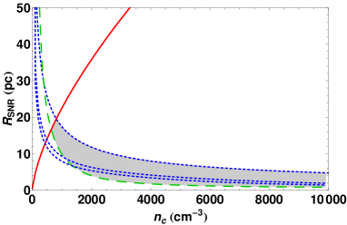
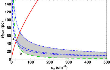
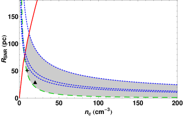
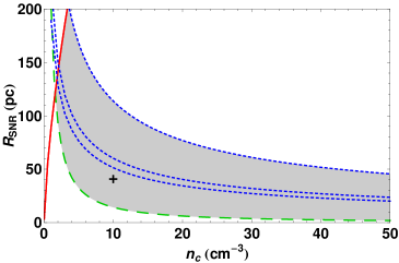
Figure 1: Constraints on the SNR radius versus cloud density for 4 different cloud radius. From top to bottom: first panel, $r_{c}$ = 1 pc; second panel, $r_{c}$ = 5 pc; third panel, $r_{c}$ = 10 pc; and forth panel, $r_{c}$ = 20 pc. Dashed (green) line: upper limit for complete cloud destruction after an encounter with an adiabatic SNR derived from Eq. (25); solid (red) line: upper limit for the shocked cloud to reach the Jeans mass derived from Eq. (17); dotted (blue) lines: upper limits for the shock front to travel into the cloud before being decelerated to subsonic velocities derived from Eq. (30) for different values of the cooling function $\Lambda(T_{sh})=10^{-25}$ erg cm³ s^-1 (lower curve), $5\times 10^{-26}$ erg cm³ s^-1 (middle curve), and $3\times 10^{-27}$ erg cm³ s^-1 (upper curve). The shaded area (between the solid, dashed and dotted lines) defines the region where star formation can be induced by a SNR-cloud interaction. The crosses and the triangle in the panels indicate the initial conditions assumed for the clouds in the numerical simulations described in Section 4.2 of Paper I (see text for details).

1. In paper I, the dotted (blue) curves of the diagrams were built for one value only of the radiative cooling function of the shocked material, i.e. $\Lambda(T_{sh})\simeq 10^{-27}$ erg cm³ s^-1 which is valid for a diffuse gas with temperature 100 K and ionization fraction $\leq$ 10^-4. Considering that the constraint established by the dotted (blue) curve is sensitive to $\Lambda(T_{sh})$ (through Eq. 30) which in turn, can vary by two orders of magnitude depending on the value of the ionization fraction of the cloud gas, we have presently plotted in the diagrams three different dotted (blue) curves in order to cover a more realistic range of possible ionization fractions from 0.1 to 10^-4, corresponding to $\Lambda(T_{sh})=10^{-25}$ erg cm³ s^-1 (lower dotted curve), $5\times 10^{-26}$ erg cm³ s^-1 (middle dotted curve), and $3\times 10^{-27}$ erg cm³ s^-1 (upper dotted curve), respectively (see Dalgarno & McCray 1972). The middle dotted (blue) curve corresponds to the average value of $\Lambda$ in the range above, $5\times 10^{-26}$ erg cm³ s^-1, and could be taken as a reference.

2. In the solution presented in Paper I for the cloud with $r_{c}=$ 1 pc (top panel of Figure 1), there was no allowed SF shaded zone. According to the present corrections and modifications, we see that a thin shaded ”star-formation unstable” zone appears now when the cooling function $\Lambda$ has values which are smaller than $10^{-25}$ erg cm³ s^-1, or ionization fractions $\mathrel{\hbox{\hbox to0.0pt{\hbox{\lower 4.0pt\hbox{$\sim$}}\hss}\hbox{$<$}}}10^{-1}$.

3. The cross labeled in the bottom panel of Figure 1 for an $r_{c}=$ 20 pc diffuse cloud corresponds to the initial conditions of the numerical simulations presented in Figure 6 of paper I (i.e., for a SNR at a distance $R_{SNR}\sim$ 42 pc from the surface of the cloud). In the paper I, that cross lies outside the unstable shaded zone just above the upper limit for a complete shock penetration into the cloud (the middle dotted, blue line of the diagram). With the present modifications, the cross now lies near the upper limit of the shaded unstable zone for values of the cooling function $\Lambda\mathrel{\hbox{\hbox to0.0pt{\hbox{\lower 4.0pt\hbox{$\sim$}}\hss}\hbox{$<$}}}10^{-25}$ erg cm³ s^-1, or ionization fractions $\mathrel{\hbox{\hbox to0.0pt{\hbox{\lower 4.0pt\hbox{$\sim$}}\hss}\hbox{$<$}}}10^{-1}$. This result remarks how sensitive the analytical diagrams are to the choice of $\Lambda$ (or the ionization fraction) for a given initial cloud temperature. According to the radiative cooling chemo-hydrodynamical simulations of Figure 6 of Paper I (which corresponds to the cross in the diagram of Fig. 1), the SNR shock front really stalls within the cloud before being able to cross it completely and, after all the shocked cloud material does not reach the conditions to become Jeans unstable, as predicted, but the dense cold shell that develops may fragment and later generate dense cores, as suggested in Paper I. This points to an ambiguity of the results due to their sensitivity to $\Lambda$ and the real ionization fraction state of the gas. We should also remark that the constraint established by the dotted (blue) curves in the diagrams is actually only an upper limit for the condition of penetration of the shock into the cloud. The condition that the mach number of the shocked material goes to $M\sim 1$ implies the pressure equilibrium between the shocked and the unshocked cloud material at the time $t_{st}$ when the shock stalls within the cloud. A quick exam of the numerical simulations of Figure 6 of Paper I, however, shows that the shock front stalls even before this balance is attained. This implies that the time $t_{st}$ could be possibly smaller and therefore, the dotted (blue) curves in the diagrams should lie below the location predicted by Eq. (30).

In spite of the important alterations above in the diagrams of Figure 1, the main results and conclusions of Paper I for interactions involving SNRs with $non-magnetized$ clouds, particularly those regarding the young stellar system $\beta$-Pictoris, have remained unchanged (see below, however, the implications for this system when the magnetic field is incorporated into the cloud).

Figure 2 shows the same diagrams as in Figure 1 except that they include the effects of the magnetic field in the cloud, as described by Eqs. 21, 27 and 30. We notice that the presence of a normal magnetic field to the shock front with an intensity of 1 $\mu$G inhibits slightly the domain of SF in the diagrams, as expected. The magnetic field plays a dominant role over the Jeans constraint (the solid (red) line in the diagrams) that causes a drift of the allowed (shaded) zone of SF to the right in the diagrams (i.e., to larger cloud densities) when compared to the diagrams without magnetic fields of Fig. 1. This drift however must be interpreted with care. When deriving the Jeans constraint in the presence of a non-null uniform magnetic field normal to the shock front (eq. 19) we assumed an one-dimensional collapse. However, although the presence of $\vec{B}$ may affect the initial compression and collapse of the shocked material, the later evolution and collapse of this material in three-dimensional space will occur mostly in the direction parallel to $\vec{B}$ and thus will not be any further affected by it. For this reason, we should expect that the actual domain of an unstable magnetized cloud in the diagrams of Figure 2 will be more extended to the left of the solid (red) line and will be ultimately bounded by the dotted-dashed (red) line that gives the Jeans constraint for a null (or parallel) magnetic field, just like in Figure 1. This part of the diagrams with non-null $\vec{B}$ will be particularly important when comparing them with the 3-D numerical simulations of cloud-SNR interactions. When larger magnetic field intensities are considered (5-10 $\mu$G) there is a significant shrinking of the allowed SF zone in the diagrams (see Figure 3). This can be understood in terms of the mass to magnetic flux ratio of the cloud before the impact. It is given by $N/B=885(n_{c,10}r_{c,10})/B_{c,6}$. This implies $B/B_{cr}\sim 0.7B_{c,6}/(n_{c,10}r_{c,10})$, which is larger than 1 for $n_{c,10}\leq 34.8$ cm^-3 and $n_{c,10}\leq 69.6$ cm^-3 for an unshocked cloud with $B=5\;\mu$G and $B=10\;\mu$G of Fig. 3, respectively, before the interaction.

As in Figure 1, the symbols (i.e., the crosses and the triangle) in Fig. 2 indicate the initial conditions assumed for the SNR-clouds interactions examined in the numerical simulations described in Paper I for unmagnetized SNR-cloud interactions. We see that when the magnetic field is included, both the crosses and the triangle lie outside the SF domain of the diagrams. This means that for the initial conditions corresponding to these points in the diagram, SF is unlikely to occur. In paper I, the application of the results of the diagram of Figure 1 for an unmagnetized cloud with $r_{c}=$ 10 pc and $n_{c}\mathrel{\hbox{\hbox to0.0pt{\hbox{\lower 4.0pt\hbox{$\sim$}}\hss}\hbox{$>$}}}$ 10 cm^-3 to the young stellar association of $\beta-$Pictoris (see the region near the cross in the third panel of Fig. 1) had led us to conclude that this stellar association could have originated from recent past interaction between a cloud and an SNR with a radius of approximately 52 pc. However, the inclusion of an effective magnetic field in the cloud with an intensity of only 1 $\mu$G has put the same cross corresponding to the initial conditions for formation of this young stellar association outside of the SF zone (see the cross in the third panel of Fig. 2).

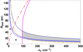
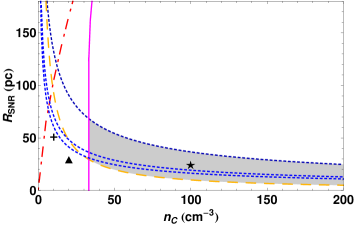
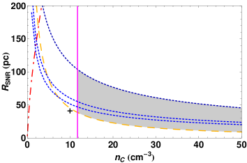
Figure 2: Constraints on the SNR radius versus cloud density for 4 different cloud radius as in Figure 1, but in the presence of a magnetized cloud with a normal B to the shock front B= 1 $\mu$G. Dashed (yellow) line: upper limit for complete cloud destruction after an encounter with an adiabatic SNR derived from Eq. (25); solid (magenta) line: upper limit for the shocked cloud to reach the Jeans mass derived from Eq. (17); dotted (blue) lines: upper limits for the shock front to travel into the cloud before being decelerated to subsonic velocities derived from Eq. (30) for different values of the cooling function $\Lambda(T_{sh}(t_{st}))=10^{-25}$ erg cm³ s^-1 (lower curve), $5\times 10^{-26}$ erg cm³ s^-1 (middle curve), and $3\times 10^{-27}$ erg cm³ s^-1 (upper curve). The dashed-dotted line (red) corresponds to the Jeans mass constraint for null magnetic field (see text for details). The shaded area defines the region where star formation can be induced by a SNR-cloud interaction (between the solid, dashed and dotted lines). The crosses and the triangle in the panels indicate the initial conditions assumed for the clouds in the numerical simulations described in Section 4.2 of Paper I. The star corresponds to the initial conditions of the MHD simulation of Figure 6.

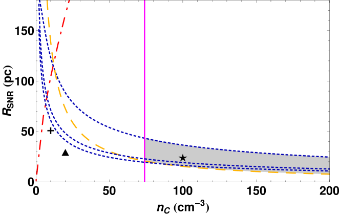
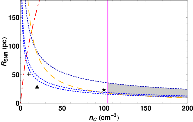
Figure 3: The same as in Figure 2 for a cloud with $r_{c}=$ 10 pc and now considering $B=5\;\mu$G (upper panel) and $B=10\;\mu$G (bottom panel).

4 SNR-cloud interaction: MHD numerical simulations of self-gravitating clouds

As remarked before, there has been several numerical studies of the impact of shock fronts on interstellar clouds (e.g., Sgro 1975; McKee & Cowie 1975; Woodward 1976; Nittmann et al. 1982; Tenorio-Tagle & Rozyczka 1986; Hartquist et al. 1986; Bedogni & Woodward 1990; Mac Low et al. 1994; Klein, McKee & Colella 1994; Anderson et al. 1994; Dai & Woodward 1995; Xu & Stone 1995; Jun, Jones & Norman 1996; Redman, Williams & Dyson 1998; Jun & Jones 1999; Lim & Raga 1999; de Gouveia Dal Pino 1999; Miniati, Jones & Ryu 1999; Poludnenko, Frank & Blackman 2002; Fragile et al. 2004; Steffen & López 2004, Raga, de Gouveia Dal Pino et al. 2002; Fragile et al. 2005; Marcolini et. al 2005; Melioli, de Gouveia Dal Pino & Raga 2005; Nakamura et al. 2006) most of which were mainly concerned with the effects of these interactions upon the destruction of the cloud. In particular, the studies that incorporated the effects of the radiative cooling revealed the relevance of it in delaying the destruction of the cloud and the mixing of its materials with the ISM (e.g., Melioli, de Gouveia Dal Pino & Raga 2005).

In paper I, in order to check the predictions of our semi-analytic diagrams built for interactions involving SNR shocks and non-magnetized clouds, we performed 3-D hydrodynamical radiative cooling simulations following the initial steps of these interactions. Here, we repeat this analysis but also take into account the effects of the magnetic fields and the self-gravity, in order to follow the late evolution of the shocked material within the magnetized clouds and check whether it suffers gravitational collapse or not, in consistence with our diagrams.

To this aim, we have employed the grid code Godunov-MHD presented in Kowal & Lazarian (2007), and tested in Falceta-Gonçalves et al. (2008), which solves the gas dynamical equations in conservative form as follows:

$$\frac{\partial\rho}{\partial t}+\mathbf{\nabla}\cdot(\rho{\bf v})=0,$$ (33)

$$\frac{\partial\rho{\bf v}}{\partial t}+\mathbf{\nabla}\cdot\left[\rho{\bf vv}+\left(p+\frac{B^{2}}{8\pi}\right){\bf I}-\frac{1}{4\pi}{\bf BB}\right]=-\rho\mathbf{\nabla\Phi},$$ (34)

$$\frac{\partial\mathbf{B}}{\partial t}-\mathbf{\nabla\times(v\times B)}=0,$$ (35)

with $\mathbf{\nabla\cdot B}=0$, where $\rho$, ${\bf v}$ and $p$ are the plasma density, velocity and pressure, respectively, ${\bf B}$ is the magnetic field and $\mathbf{\nabla^{2}\Phi}=4\pi G\rho$. The equations are solved using a second-order Godunov scheme, with an HLLD Riemann solver to properly consider the MHD characteristic speeds. For the self-gravity term, we used the FACR (Fourier Analysis Cyclic Reduction) Poisson solver at each time step. In Paper I, given the importance of the radiative cooling behind the shocks, we simulated explicitly its effects in the hydrodynamical simulations then presented. Presently, since the main focus in the simulations is to study the role of the magnetic field and self-gravity on the evolution of the clouds, we solved the equations under the approximation of strong radiative cooling. The set of equations above is closed by the equation of state $p\propto\rho^{\gamma}$, setting an effective $\gamma_{eff}=1.2$ to simulate the strong radiative cooling.

Table 1: Description of the simulations

$n_{c}$ (cm-3)	$r_{c}$ (pc)	$R_{SNR}(pc)$	code	$B$ ($\mu$G)	Result	Prediction
10	20	40	Hydro	-	collapse	collapse
10	20	40	MHD	1	stable	stable
50	5	15	MHD	1	stable	stable
10	10	50	MHD	1	stable	stable
100	10	25	MHD	1	collapse	collapse

The computational box has dimensions 100 pc $\times$ 100 pc $\times$ 100 pc, corresponding to a fixed mesh of 256³ grid points. A SNR is generated by the explosion of a SN with energy $E_{0}=10^{51}$ erg initially injected at the left-bottom corner of the box. Several runs were carried out with different initially uniform cloud densities ($n_{c}$), radii ($r_{c}$), and distance between the SNR and the cloud’s surface ($R_{SNR}$). The initial conditions are described in Table 1. We have selected two of these simulations to show in detail, as follows.

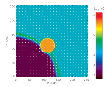
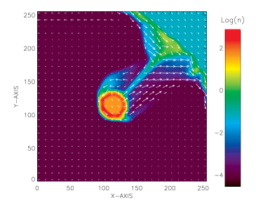
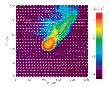
Figure 4: Colour-scale maps of the mid-plane density distribution and magnetic field vectors evolution for the model with $n_{c}=10$ cm^-3, $r_{c}=10$ pc, $R_{SNR}=50$ pc, and $B=1\mu$G. The evolutionary times are $t=3\times 10^{5}$yr (top left-hand panel); $8\times 10^{5}$yr (top right-hand panel); $1.8\times 10^{6}$yr (bottom left-hand panel); and $3.3\times 10^{6}$yr (bottom right-hand panel).The ISM where the SNR expands has a number density $n=0.05$ cm^-3, and a temperature $10^{4}$ K. The field vectors are normalized by the maximum at each frame.

Fig. 4 depicts the maps of the density and magnetic field vectors at the mid x-y plane that intercepts both the cloud and de SNR for a cloud with $n_{c}=10$ cm^-3, $r_{c}=10$ pc, $R_{snr}=50$ pc. These initial conditions represent the cross at the third panel of Fig. 2 (from top to bottom) which lies well outside of the SF shaded zone in the diagram and predicts cloud destruction due to the impact. In the simulation of Fig. 4, the SNR shock front compresses the cloud increasing the magnetic energy density. After the interaction (at $t\simeq 1.8\times 10^{6}$ s, a tail of gas is swept behind the cloud by the expanding SNR, similarly to the results obtained, e.g., by Murray et al. (1993). The magnetic energy density along the tail is also increased. We see that, due to the compression, the cloud initially becomes gravitationally unstable and starts to collapse. At $1.8\times 10^{6}$yr, the core is $\sim 10^{3}$ times denser. The contraction of the cloud also causes the increase of the magnetic energy that acts against further collapse. Later, the simulated cloud rebounds and undergoes expansion and evaporation, as seen at $3.3\times 10^{6}$yr. This re-expansion may be occurring mostly because of the inefficient cooling of the simulation. Since we set $\gamma_{eff}=1.2$ the gas may be not being realistically cooled, as one should expect for a real ISM collapsing cloud. In such situations, $\gamma_{eff}$ may be even smaller than unity, i.e. the shocked material may present temperatures lower than right before the shock. On the other hand, Spaans & Silk (2000) modeled the chemistry, thermal balance and radiative transfer for different conditions of the ISM, and showed that a polytropic pressure equation may be used as first approximation. The effective polytropic index is $\gamma_{eff}\sim 0.8-1.4$, depending on the local conditions. Nonetheless, even though the real cloud would not re-expand in the presence of a stronger radiative cooling, the non-collapsing condition is still possible due to the increase in the magnetic energy. In any case, we are currently implementing a more realistic method to calculate the cooling function in our Godunov-MHD code, based on the interpolation method for a table of $\Lambda(T)$ parameter (see Stone et al. (2008)). We intend to compare the presented results with more realistic calculations in a forthcoming work.

In Paper I, where non-equilibrium radiative cooling has been properly taken into account, but no magnetic field or self-gravity were considered, the hydrodynamical simulations (Fig. 4 of that paper) suggest that the cloud evaporates. As the magnetic field is introduced (Fig. 4 of the present paper) the increasing magnetic pressure at the later stages of the cloud evolution prevents the collapse, as predicted by the SF diagram of Fig. 2.

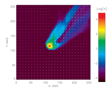
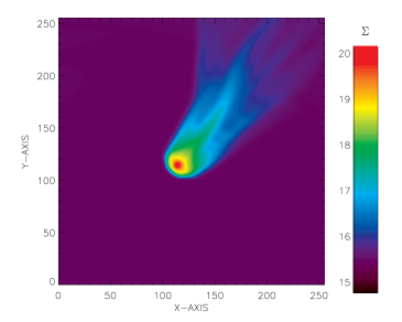
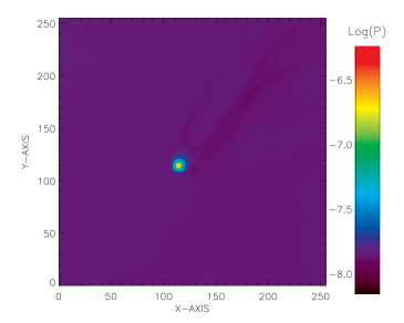
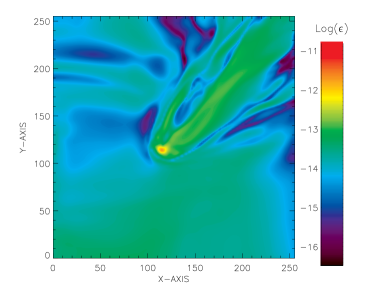
Figure 5: Colour-scale maps of the mid-plane density with magnetic field vectors, column density, gas pressure and magnetic energy density for the same model as in Figure 4 at $t=1.8\times 10^{6}$yr.

Figure 5 shows the distribution of several physical parameters of the model of Fig. 4 at $t=1.8\times 10^{6}$ yr. The column density is $N>10^{20}$ cm^-2 in the core. As remarked above, we see that the dense core formed during the initial collapse results an increase of the total gas and magnetic pressures with a maximum temperature $T>10^{4}$ K, while the magnetic energy density is an order of magnitude larger than that of the surrounding medium. The large increase of the gas pressure is probably the main responsible for the re-expansion of the cloud. This is highly dependent on the radiative cooling. In a more realistic situation, the cooling timescale $t_{cool}\sim kT/n\Lambda(T)$ should be generally shorter than the collapsing timescale $t_{g}\sim(G\rho)^{-1}$, which means that the core temperature should be smaller than $10^{4}$K. Nevertheless, the magnetic field also plays a crucial role in stabilizing the cloud and supporting the cloud against collapse, as discussed below in Fig. 7.

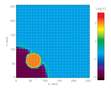
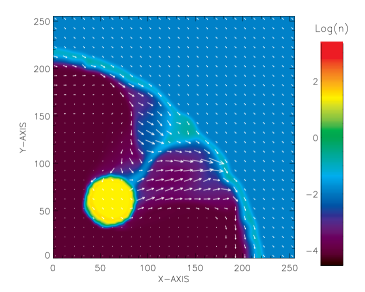
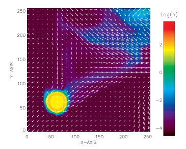
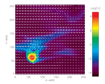
Figure 6: Colour-scale maps of the mid-plane density distribution and magnetic field vectors for the model with $n_{c}=100$ cm^-3, $r_{c}=10$ pc, $R_{SNR}=25$ pc, and $B=1\mu$G. The evolutionary times are $t=2\times 10^{5}$ yr (top left-hand frame); $5\times 10^{5}$ yr (top right-hand frame); $1.2\times 10^{6}$yr (bottom left-hand frame); and $2.5\times 10^{6}$ yr (bottom right-hand frame). The vectors are normalized by the maximum at each frame.

Figure 6 shows the mid-plane maps of the density distribution and the magnetic field vectors for the model of Table 1 with a cloud with $n_{c}=100$ cm^-3 and $r_{c}=10$ pc, and a SNR with $R_{SNR}=25$pc. The evolution in this case is similar to the previous model. However, after $t=1.2\times 10^{6}$yr, as the cloud collapses the magnetic pressure is not able to counter-balance gravity and the cloud keeps contracting. The higher cloud density in this case causes an efficient radiative cooling of the shock compressed material in the cloud that keeps the thermal energy low. Thus the collapse simply drags the magnetic field lines that increase the magnetic energy density, but this will never be able to stop the collapse. This result is consistent with the predictions of the SF formation diagram. The initial conditions of this system of Fig. 6 correspond to the star symbol at the third panel of Fig. 2 (from top to bottom) which lies inside the SF shaded zone.

As remarked before, the stability of a cloud supported by the magnetic pressure may be quantified by the mass-to-magnetic flux ratio, $M/\Phi\simeq N/B$, where N is the cloud column density (e.g., Crutcher 1999). We have computed this mass-to-flux ratio for the simulated clouds above at several time-steps. The results are shown in Figure 7. The open dots represent the maximum column density for each snapshot as a function of the magnetic field averaged along the given line of sight (with maximum $N$). We notice that for the model with $n_{c}=10$ cm^-3, $r_{c}=10$ pc and $R_{SNR}=50$ pc (of Fig. 4), the cloud starts collapsing right after the interaction with the SNR. The column density increases and reaches the unstable regime. The cloud contracts and the total energy increases. Both the internal and the magnetic energy densities suppress further collapse and then the cloud re-expands. Despite of the probably unrealistic re-expansion, as discussed before, the final stage is a stable cloud. For the case of $n_{c}=100$ cm^-3, $r_{c}=10$ pc, and $R_{SNR}=25$ pc, the same process occurs initially. However, the increase of the magnetic and internal energy densities are not enough to avoid the continuous collapse.

Figure 7: Mass-to-flux relation obtained for several time-steps of the simulations described in the text, for cloud conditions $n=10$ cm^-3, $r_{c}=10$ pc, $R_{SN}=50$ pc (left), and $n=100$ cm^-3, $r_{c}=10$ pc, $R_{SN}=25$ pc (right). The solid line in each diagram gives the critical mass to flux ratio which separates the gravitational unstable (on the right-hand side of the line) from the stable domain (left-hand side of the line).

The other simulated models of Table 1 have presented results which are also consistent with the SF diagrams. The first model of the table is a pure hydrodynamical system with no magnetic field whose initial conditions correspond to the cross labeled in the bottom panel of Fig. 1. According to Table 1, the numerical simulation of the evolution of this SNR-cloud interaction including the effects of self-gravity leads to the gravitational collapse of the cloud, which is in agreement with the prediction of the SF diagram. When a magnetic field of 1 $\mu$G is included in a system with the same initial conditions, the MHD numerical simulation shows that the magnetic pressure prevents the cloud collapse (second model of Table 1). This model is represented by the cross in the bottom panel of Fig. 2 which consistently lies outside the gravitational unstable zone of the diagram.

The third model of Table 1 also lies outside the unstable shaded zone of the SF diagram (see the $X$ symbol in the second panel of Fig. 2), and the MHD numerical simulation of the evolution of this system shows that the cloud ends up evaporating due to the strong SNR shock interaction.

5 Application to isolated regions of the ISM

We can apply the simple analytical study above to isolated star formation regions of our own galaxy. In paper I, we focused on the formation of the young stellar association of $\beta-$Pictoris induced by a SNR-cloud interaction. Here, we will address few other examples in our ISM that present some evidence of recent past interactions with SNRs, like the Large CO Shell in the direction of Cassiopea (Reynoso & Mangum 2001) and the so called Edge Cloud 2 in the direction of Scorpious (Ruffle et al. 2007, Yasui et al. 2006). A counter example is the region apparently without star formation around the Vela SNR. In fact, we will see below that the conditions of this region correspond to a point in our diagrams that lies outside the shaded SF zone.

The Large CO shell is an expanding structure with a velocity $\sim 3\;km/s$, a mass of $9.3\times 10^{5}\;\rm M_{\odot}$ and a density of $\sim 35\;\rm cm^{-3}$. Reynoso & Mangum (2001) suggest that this expanding structure has probably originated from the explosion of a SN about $\sim 4\times 10^{6}$ yr ago. Assuming that the cloud mass was originally uniformly distributed within a sphere of radius of 435” ($\sim 50$ pc), the initial density could be $n_{c}\simeq 30\;\rm cm^{-3}$. The SN shock front possibly induced the formation of the O 9.5 type star that has been detected as an IR source (IRAS 17146-3723). The Large CO Shell has an external radius of $50$ pc and an inner radius of $\sim 28$ pc (Reynoso & Mangum, 2001). The age and small expansion velocity suggest that it is now a fainting evolved SNR. If we consider a cloud with the above density and radius ($\sim$ 50 pc) at the time of the potential interaction with SNR in the adiabatic regime, we can identify this system in the SF diagram within the shaded zone, as indicated in Figure 8, if the SNR had a radius between $2.5-72$ pc and an ambient medium density $n\simeq$ 1 cm^-3. However, when we include a magnetic field in the cloud of $1\;\mu$G, the range of possible radii for the SNR is reduced to $R_{SNR}\sim 7.8-72$ pc if the maximum radius is calculated using a radiative cooling function $\Lambda=3\times 10^{-27}$ erg cm³ s^-1. For an average $\Lambda$ $=5\times 10^{-26}$ erg cm³ s^-1, the maximum possible radius of the SNR is reduced to 38.4 pc. Considering that the present radius of the evolved SNR is probably around 50 pc, the range above of initial conditions for the SNR-cloud interaction is quite plausible.

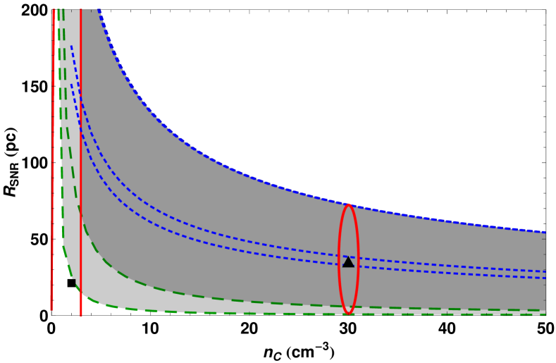
Figure 8: Diagram presenting the parameter space domain for SF for a cloud interaction with a SNR in the adiabatic regime. The light-gray shaded zone corresponds to the allowed SF zone for the interaction without magnetic field while the dark-gray corresponds to the interaction with the magnetized cloud with $B=1\;\mu$G. As in the previous figures, the dotted (blue) lines from top to bottom represent the shock penetration constraint for three different values of $\Lambda=3\times 10^{-27}\;\rm erg\;cm^{3}\;s^{-1}$; $5\times 10^{-27}\;\rm erg\;cm^{3}\;s^{-1}$; and $1\times 10^{-25}\;\rm erg\;cm^{3}\;s^{-1}$, respectively. The other initial conditions are $r_{c}=$ 50 pc and $T_{c}=100\;\rm K$. The ambient medium density is $n=$ 1 cm^-3. The triangle represents the average conditions for the interaction involving the Large CO Shell, centered at $n_{c}=$ 30 cm^-3 and $R_{SNR}=$ 36 pc, while the (red) ellipse indicates a possible range of values for the interacting SNR radius. The square represents the initial conditions for Vela system (see text for details).

The SNR Vela has an almost spherical, thin HI shell expanding at a velocity of $\sim 30\;km/s$. Instead of impinging on an interstellar cloud, it is expanding in a fairly dense environment with evidence of some structure formation. Assuming that Vela is at a distance of $\sim 350$ pc from the Sun, its shell radius is of the order of 22 pc. The ambient density is $\sim$ 1 to 2 $\rm cm^{-3}$ and the initial energy of the SN was around $1-2.5\times 10^{51}\;\rm erg$ (Dubner et al. 1998). These initial conditions correspond to the square symbol in the diagram of Figure 8 and it lies outside the SF shaded zone. This is consistent with the absence of dense clouds, clumps, filaments, or new born stars in the neighborhood of this SNR.

The SF region in the neighborhood of the Edge Cloud 2 is a possible example involving an interaction of a SNR in the radiative phase with a cloud. This is actually a giant molecular cloud with a diameter $\sim 30-40$ pc. It is one of the most distant cloud complexes from the galactic center of the Milky Way ($d\simeq$ $22-28$ kpc; Ruffle et al. 2007). For this reason, it is embedded in a region where the gas pressure is extremely small and the presence of external SF agents like spiral arm perturbations is improbable. This could be an indication that this cloud complex is very stable, except for the recent detection of two associations of T-Tauri stars with ages of $\sim 10^{6}$ yr (Kobayashi & Tokunaga 2000, Yasui et al. 2006). The Edge 2 cloud has a temperature of $20$ K, a density $n_{H_{2}}\sim 10^{4}$ cm^-3, and an estimated mass of $\sim 10^{4}\;M_{\odot}$. There is an old and large SNR associated to this cloud, GSH 138-01-94, which consists of an HI shell with a radius of $180$ pc expanding into the ISM with a speed of $11.8\pm 0.9$ km/s and an age of about $4.3\times 10^{6}$ yr (Ruffle et al. 2007). According to Ruffle et al. (2007), the formation of the present structure and chemical composition of the Edge 2 Cloud is possibly a result of interactions of this SNR with the IS gas.

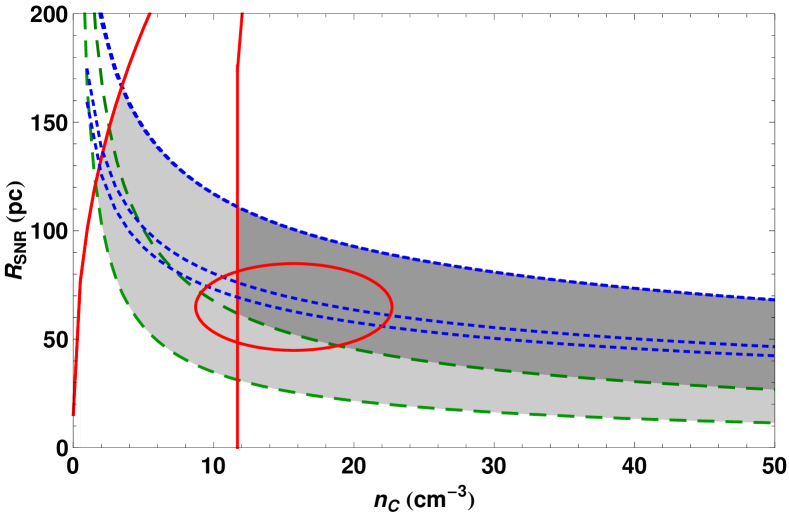
Figure 9: Diagram presenting the parameter space domain for SF for a cloud interaction with a SNR in the radiative regime expanding in an ambient medium with $n\sim 0.14$ cm^-3. The light-gray shaded zone corresponds to the allowed SF zone for the interaction without magnetic field while the dark-gray corresponds to the allowed SF zone for the interaction with the magnetized cloud with $B=1\;\mu$G. As in the previous Figures, the dotted (blue) lines from top to bottom represent the shock penetration constraint for three different values of $\Lambda=3\times 10^{-27}\;\rm erg\;cm^{3}\;s^{-1}$; $5\times 10^{-27}\;\rm erg\;cm^{3}\;s^{-1}$; and $1\times 10^{-25}\;\rm erg\;cm^{3}\;s^{-1}$, respectively. The other initial conditions are $r_{c}=20$ pc and $T_{c}=100$ K which are appropriate for the Cloud 2$-$SNR GSH 138-01-94 system. The ellipse indicates a possible range in the parameter space for the interaction between the Edge Cloud 2 and the SNR to result in gravitational collapse. It spans the ranges $n_{c}\simeq 9.4-22$ cm^-3 and $R_{SNR}\simeq 46-84$ pc.

Considering the SNR characteristics above (i.e., its velocity, radius and an energy $\sim 10^{51}$ erg) and using Eq. 8 of the Paper I, we can estimate an ambient density $n\sim 0.14$ cm^-3. Also, assuming that the mass of the cloud was originally distributed uniformly in a sphere of average radius $\sim 17.5$ pc, we find that the density of the cloud before the compression was $n_{c}\sim 14\;\rm cm^{-3}$. With these initial conditions, the SNR-cloud interaction would lie within the allowed SF zone of the diagram of Figure 9 for a SNR with a radius between $\sim$ 31 and 102 pc at the time of the interaction and for a value of $\Lambda=3\times 10^{-27}$erg cm³ s^-1. We can try to constrain further the possible value of the radius of the SNR assuming that the interaction started sometime after the remnant had become radiative and before $10^{6}$ yr, which is the approximate age of the observed stars. These limits imply $R_{SNR}\simeq$ $46$ pc - $84$ pc, as indicated by the region within the ellipse in the diagram of Figure 9.

6 Estimating the efficiency of star formation from SNR-cloud interactions

In the study we have carried out here, we concentrated on isolated interactions between diffuse clouds and SNRs without focusing on the effects that such interactions can have upon the global SF in the Galaxy. The present star formation efficiency is typically observed to be very small, of the order of a few 0.01 in dispersed regions, but it can attain a maximum of $\sim 0.3$ in cluster-forming regions (Lada & Lada 2003; see also Nakamura & Li 2006 for a review).

From the present analysis, we can try to estimate the star formation efficiency that interactions between SNRs and diffuse clouds produce and compare with the observed values in order to see the contribution of this mechanism on the overall SFE in the Galaxy. The diagrams built in this work provide a SF domain for these interactions, in other words, they establish a set of conditions that isolated interactions must satisfy in order to result in successful gravitational collapse of the compressed cloud material. In order to evaluate the corresponding global SFE of these interactions we have to calculate first their probability of occurrence in the Galaxy. Considering that once a SNR is formed it will propagate and compress the diffuse medium around it providing the sort of interactions we are examining, the probability of these interactions to occur must be proportional to:

$$f_{SNR}\simeq N_{SNII}\Delta t_{SNR}(R_{SNR})\frac{A_{SNR}(R_{SNR})}{A_{G}}$$

$$\simeq 10^{-1}\ {{N_{SNII}}\over{1.7\times 10^{-2}\rm s}}\;{{\Delta t_{SNR}}\over{5\times 10^{5}\rm s}}\;{{A_{SNR}}\over{2.5\times 10^{3}pc^{2}}}\;{{A_{G}}\over{4\times 10^{8}pc^{2}}}$$ (37)

Where we have assumed a homogeneous galactic thin disk with a radius of 20 kpc to compute the galactic area ($A_{G}$), and where $N_{SNII}$ is the rate of SNII explosions (e.g. Cappellaro, Evans & Turatto 1999), $\Delta t_{SNR}(R_{SNR})$ is the lifetime and $A_{SNR}$ is the area of a SNR and both depend on $R_{SNR}$. Since not all the galactic volume is filled up with clouds, this quantity above must be multiplied by the diffuse neutral clouds filling factor in order to give the approximate probability of occurrence of SNR-clouds interactions. If we consider the amount of gas that is concentrated within cloud complexes in the cold phase of the ISM, the corresponding volume filling factor of the clouds is $f_{c}\simeq 5\%$ (e.g., de Avillez & Breitschwerdt 2005), and then the probability of occurrence of the interactions will be given by $f_{SNR-c}\simeq f_{SNR}\times f_{c}$. Substituting Eq. (2) and (6) for $\Delta t_{SNR}(R_{SNR})$ of Paper I in Eq. (37) we find:

$$f_{SNR-c}(R_{SNR},a)=f_{SNR}\times f_{c}\simeq 9.5\times 10^{-3}\;R_{SNR,50}^{9/2}$$

for an interaction with a SNR in the adiabatic regime and

$$f_{SNR-c}(R_{SNR},r)=2.9\times 10^{-3}\;R_{SNR,50}^{11/2}$$

for an interaction with a SNR in the radiative regime.

This probability can be multiplied by the mass fraction of the shocked gas that is gravitationally unstable within the SF domain of our SNR-cloud interaction diagrams in order to give an effective global star formation efficiency for these interactions. Using the calculated Jeans mass for the shocked gas (Eqs. 15, 16 and 20) as an approximate lower limit for the mass fraction of the cloud that should collapse to form stars, we obtain:

$$sfe_{SNR-c}\simeq f_{SNR-c}\frac{m_{J}}{m_{c}}$$

which in the case of a non-magnetized cloud interacting with a SNR in the adiabatic regime gives (according to Eq. 15):

$$sfe_{SNR-c,a}\simeq 5.4\times 10^{-3}\frac{T_{c,100}^{2}\;R_{SNR,50}^{6}}{\;n_{c,10}\;r_{c,10}^{3}\;E_{51}^{1/2}\;I_{5}}$$ (38)

And for the case of the interaction of a non-magnetized cloud with a SNR in the radiative phase (using Eq. 16):

$$sfe_{SNR-c,r}\simeq 1.5\times 10^{-3}\frac{T_{c,100}^{2}\;R_{SNR,50}^{6}\;n^{0.41}}{\;n_{c,10}\;r_{c,10}^{3}\;I_{5}\;E_{51}^{0.8}f_{10}^{1/2}}$$ (39)

For the interaction involving a magnetized cloud we have:

$$sfe_{SNR-c,B}\simeq\frac{5\;f_{SNR-c}(R_{SNR})}{\;y^{1/2}\;n_{c,10}^{3/2}\;r_{c,10}^{3}}\left[4.14\;T_{c,100}+\frac{4\;y\;B_{6}^{2}}{n_{c,10}}\right]^{3/2}$$ (40)

where $y$ must be substituted by Eq. 8. Using Eqs. 9 and 48 it gives the sfe for interactions with adiabatic SNRs and using Eqs. 10 and 49 it gives the sfe for interactions with radiative SNRs.

As examples, Figures 10 and 11 show plots of the approximate sfe computed for SNR-clouds interactions as a function of the SNR radius for different values of the cloud magnetic field and for different values of the cloud density. Since the computed sfe is already dependent of the Jeans mass constraint (see Eqs. 38 and 39), the zone that defines the allowed SF domain in these new plots is constrained by the other two conditions over $R_{SNR}$, i.e., the shock penetration into the cloud and the cloud non-destruction conditions calculated in Section 3. The increase of the magnetic field tends to shift the SF zone to smaller values of the radius of the SNR both for SNRs in the adiabatic and in the radiative regimes. The vertical line in the diagrams establishes the transition radius of the SNR from the adiabatic (left) to the radiative (right) regime for the specific initial conditions of the diagrams. In other words, the relevant domain in the diagrams of Figure 10 is on the left-hand side of this line, while in Fig. 11, it is on the right-hand side.

We note that the effective sfe found for these interactions is generally smaller than the typical values observed for the Galaxy and the range of possible values for sfe decreases with the increase of the magnetic field in the cloud. We also see that the parameter space that allows sfe values close to the observed values (0.01$-$0.3) is very reduced. The diagrams of Fig. 11, which appy to interactions involving more evolved SNRs already in the radiative phase, shows interesting results. In this phase the SNR is less powerful and therefore, less destructive than in the adiabatic phase. Besides, it is much more expanded increasing the probability of encounters with clouds. This explains the larger attained values of the calculated $sfe_{SNR-c}$. However, the parameter space that allows successful interactions for SF on the right-hand side of the diagrams is even thinner than in the interactions with adiabatic SNRs (Fig. 10) and disappears when $B_{c}=10\;\mu$G.

The results above suggest that these interactions are not sufficient to explain the observed sfe of the Galaxy either in the presence or in the absence of the magnetic field in the cloud. They are consistent with previous analysis performed by Joung & Mac Low (2006) where these authors have concluded that Supernova-driven turbulence tends to inhibit global star formation rather than triggering it. We should note however, that they have based their conclusion on the computation of the star formation rate (SFR), rather than the sfe, from box simulations of the ISM with SN turbulence injection and their computed SFR has been weighed by a fixed value of the sfe taken from the observations (sfe $\sim$ 0.3).

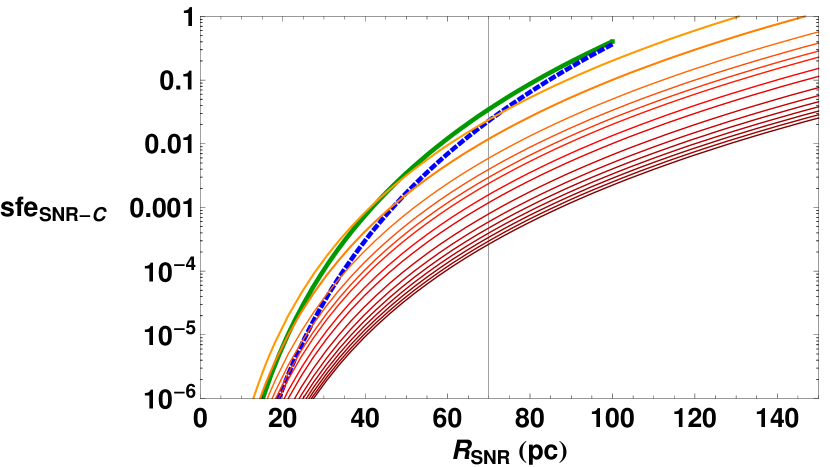
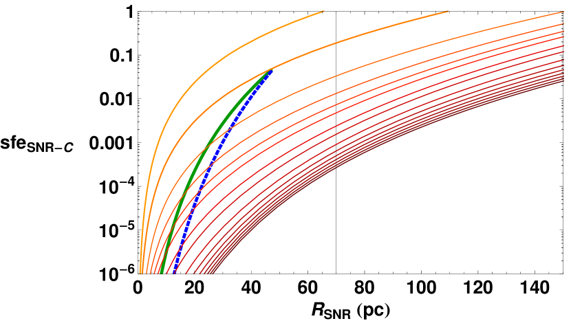
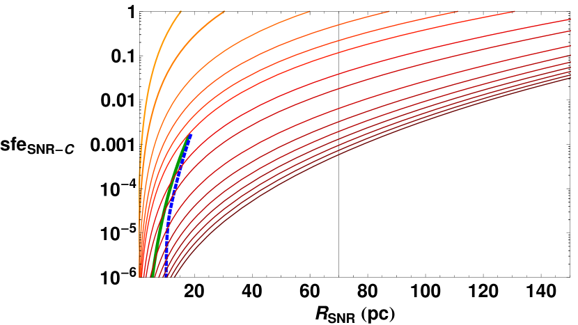
Figure 10: Plots of the calculated star formation efficiency as a function of the SNR radius in the adiabatic regime for several values of the cloud density represented by the continuous (reddish) lines (from top to bottom: 10, 20, 40, 60, 80, 100, 150, 200, 300, 400, 500, 600, 700, 800, 900 $\rm cm^{-3}$) for an interaction with a cloud with: (a) $B_{c}=0$ (top panel); (b) $B_{c}=1\;\mu$G ( middle panel); and (c) $B_{c}=10\;\mu$G (bottom panel). The other initial conditions are $r_{c}=10\;\rm pc$, $T_{c}=100\;\rm K$, and $\Lambda=5\times 10^{-26}$ erg cm³ s^-1. The ambient medium density used is $n=0.05$ cm^-3. The two constraints, i.e., the non-destruction condition of the cloud (solid, green line) and the shock penetration condition (dotted, blue line) delineate the zone for allowed SF in these sfe versus $R_{SNR}$ diagrams. The continuous vertical (black) line represents the transition radius of the SNR from the adiabatic to the radiative regime so that only the values of $R_{SNR}$ on the left-hand side of this line are relevant in these diagrams (see text for details).

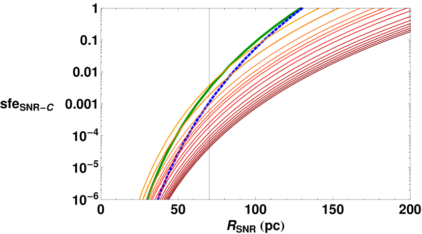
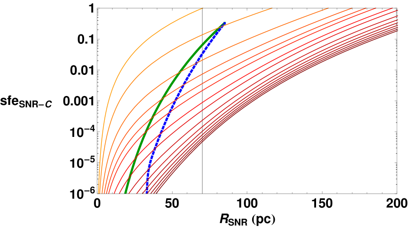
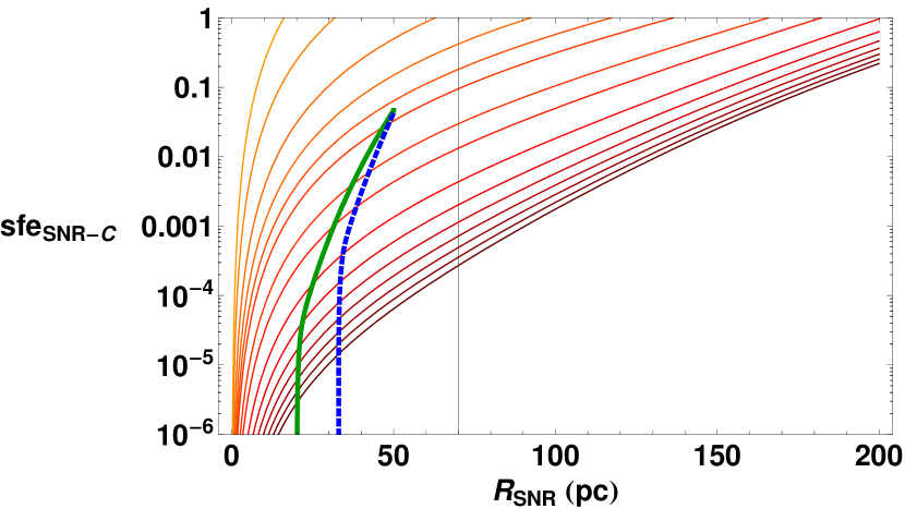
Figure 11: The same as in Figure 10, but considering the interaction with a SNR in the radiative phase. In these diagrams, only the values of $R_{SNR}$ on the right-hand side of the vertical (black) line are relevant in this phase.

7 Conclusions

We have presented here a study of isolated interactions between SNRs and diffuse neutral clouds focusing on the determination of the conditions that these interactions must satisfy in order to lead to gravitational collapse of the shocked cloud material and to star formation, rather than to cloud destruction. A preliminary study of these interactions neglecting the effects of the magnetic field in the cloud had been performed previously by Melioli et al. (2006). We have presently incorporated these effects and derived a new set of conditions for the interactions. A first condition determines the Jeans mass limit for the compressed cloud material in the impact. A second one establishes the penetration extent of the SNR shock front inside the cloud before being stalled due to radiative losses. It must have energy enough to compress as much cloud material as possible before fainting. A third constraint establishes the condition upon the same shock front under which it will $not$ become too strong to destroy the cloud completely. We have then built diagrams of the radius of the SNR as a function of the cloud density where this set of constraints delineate a domain within which star formation may result from these SNR-cloud interactions (Section 3). As expected, we find that an embedded magnetic field in the cloud normal to the shock front with an intensity of 1 $\mu$G inhibits slightly the domain of SF in the diagram when compared to the non-magnetized case. The magnetic field plays a dominant role over the Jeans constraint causing a drift of the allowed SF zone to higher cloud densities in the diagram. When larger intensities of magnetic fields are considered (5-10 $\mu$G), the shrinking of the allowed SF zone in the diagrams is much more significant. We must emphasize however that, though observations indicate typical values of $B_{c}\simeq 5-10\mu$G for these neutral clouds, the fact that we have assumed uniform, normal fields in the interactions have maximized their effects against gravitational collapse. We should thus consider as more realistic the result obtained when an effective $B_{c}\simeq 1\mu$G was employed. These diagrams derived from simple analytical considerations provide a useful tool for identifying sites where star formation could be triggered by the impact of a SN blast wave.

We have also performed fully 3D MHD numerical simulations of the impact between a SNR and a self-gravitating cloud for different initial conditions (Section 4) tracking the evolution of these interactions and identifying the conditions that have led either to cloud collapse and star formation or to complete cloud destruction and mixing with the ambient medium. We have found the numerical results to be consistent with those established by the SNR-cloud density diagrams, in spite of the fact that the later have been derived from simplified analytic theory. We remark that the radiative cooling in the MHD numerical simulations has been considered through the adoption of an approximate polytropic pressure equation with $\gamma_{eff}\sim 1.2$ (see Spaans & Silk 2000). We are presently implementing a more realistic cooling function in our Godunov-MHD code in order to test, e.g., the re-expanding cloud case and its validity under more realistic situations.

We have applied the results above to a few examples of regions in the ISM with some evidence of interactions of the sort examined in this work. In paper I, the application of the results of the $SF$ diagram for a non-magnetized cloud (as in Figure 2) to the conditions around the young stellar association of $\beta-$Pictoris in our local ISM had led us to conclude that this stellar association could have originated from past cloud-SNR interaction only under very restrict conditions, i.e., with a cloud with radius $\sim$ 10 pc and density $\sim$ 20 cm^-3 and a SNR with a radius $\sim$ 42 pc. However, in the present work we find that with the inclusion of an effective magnetic field in the cloud with an intensity of only 1 $\mu$G this interaction is unlikely to produce that stellar association (Figure 2, cross in the third panel from top to bottom), at least not for the set of initial conditions proposed in the literature for that system (see also Melioli et al. 2006). In the case of the expanding Great CO Shell$-$O9.5 star system, we find that local star formation could have been induced in this region if, at the time of the interaction, the SNR that probably originated this expanding shell was still in the adiabatic phase and a radius between $\sim$ 8 pc $-$ 29 pc impinged a magnetized cloud with density around 30 $\rm cm^{-3}$ (Figure 8). Another example is the SF region near the Edge Cloud 2. This is one of the most distant cloud complexes from the galactic center where external perturbations should thus be rare. But the recent detection of two young associations of T-Tauri stars in this region could have been formed from the interaction of a SNR in the radiative phase with a cloud, if the interaction started $\mathrel{\hbox{\hbox to0.0pt{\hbox{\lower 4.0pt\hbox{$\sim$}}\hss}\hbox{$<$}}}10^{6}$ yr, the SNR had a radius $R_{SNR}\simeq$ $46$ pc $-$ $84$ pc and the magnetized cloud a density around $n_{c}\sim 14\;\rm cm^{-3}$ (Figure 9).

Finally, though in this study we have focused on isolated interactions involving SNRs and clouds, we used the results of the diagrams to estimate the contribution of these interactions to global star formation. Our evaluated effective star formation efficiency for this sort of interaction is generally smaller than the observed values in our own Galaxy (sfe $\sim$ 0.01$-$0.3) (Figures 10 and 11). This result seems to be consistent with previous analysis (e.g., Joung & Mac Low 2006) and suggests that these interactions are powerful enough to drive structure formation, supersonic turbulence (see, e.g., simulation of Figure 4) and eventually ”local” star formation, but they do not seem to be sufficient to drive $global$ star formation in our galaxy or in other normal star forming galaxies, not even when the magnetic field in the neutral cloud is neglected. In conclusion, the small size of the allowed SF domain in the diagrams and the results for the estimated sfe indicate that these interactions must lead more frequently to the destruction of the clouds, rather than to their gravitational collapse.

Appendix A

For spherical SNR$-$cloud interactions we need to consider the effects of curvature in the cloud-SNR interactions. The instantaneous velocity of the shocked gas moving towards the center of the cloud, $v_{cs}$, is only a fraction of the SNR velocity and depends on the density contrast, $\chi$, between the shell and the cloud (as in the planar shock case) and the angle $\gamma$ between the SNR velocity vector and the line that links the center of the cloud and the instantaneous contact point between the cloud and the SNR (Fig. 12). We see that at $t=0$, i.e, when the SNR touches the cloud, these two lines are coincident and $\gamma=0$, then $v_{cs}=\chi^{0.5}v_{SNR}$. Later, at a time $t_{c,SNR}$ when the SNR approaches the center of the cloud and the SNR shock energy input ends, $\gamma=\pi/2$ and $v_{cs}=0$ . The average value of the velocity integrated over this SNR crossing time, is

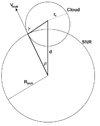
Figure 12: Schematic diagram of the interaction between an SNR and a cloud. The SNR expands and impacts the cloud. The angles $\beta$ and $\gamma$ are functions of the time, the SNR velocity, and the cloud and SNR radii, as indicated by the equations of the text.

$${\hat{v}}_{cs}\simeq v_{SNR}\ \left({{n_{sh}}\over{n_{c}}}\right)^{0.5}\ {2\over t_{c,SNR}}\ \int^{t_{c,SNR}}_{0}{\cos\gamma(t)\ dt}$$ (41)

where

$$\cos\gamma(t)\;=\frac{d^{2}-R_{SNR}^{2}(t)-r_{c}^{2}}{2R_{SNR}(t)\;r_{c}}\;,$$ (42)

$d$ is the distance between the SNR center and the cloud center, $R_{SNR}$ is the SNR radius, $r_{c}$ is the cloud radius, $n_{c}$ is the initial cloud density, $n_{sh}$ is the SNR shell density and $v_{SNR}$ is the expansion velocity of the SNR.

We assume that the distance between the center of the cloud and that of SNR remains constant:

$$d=R_{SNR}+r_{c}$$ (43)

After a time $t_{c,SNR}$, this distance can be written as

$$d=\sqrt{R_{SNR}(t)^{2}+r_{c}^{2}}$$ (44)

At this time, the SNR radius is approximately:

$$R_{SNR}(t)\simeq R_{SNR}+v_{SNR}\;\;t_{c,SNR}\;\;.$$

Thus:

$$t_{c,SNR}\simeq\frac{\sqrt{R_{SNR}^{2}+2r_{c}\;R_{SNR}}-R_{SNR}}{v_{SNR}}\;,$$ (45)

where

$$R_{SNR}=R_{SNR}(0)\;.$$

With the integration limits above, eq. (41) has a solution that should replace the more approximate one given in Paper I.

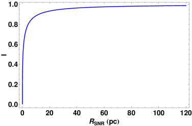
Figure 13: Values of I for a cloud with $r_{c}=$ 10 pc and for different values of $R_{SNR}$

Figure 13 depicts the plot of the integral term of eq. (41), $I={2\over t_{c,SNR}}\ \int^{t_{c,SNR}}_{0}{\cos\gamma(t)\ dt}$, for a cloud with $r_{c}=10$ pc as a function of $R_{SNR}$. It clearly shows that the effect of curvature will be relevant only for values of $R_{SNR}/r_{c}$ near unity. The corrections in the solution above to $\hat{v}_{cs}$ will produce a few changes in the multiplying factors that appear in Equations (13) to (26) of Paper I (in the absence of magnetic field), as indicated below:

$$t_{cc,a}\sim 4.7\times 10^{5}\;\frac{n_{c,10}^{0.5}\;r_{c,10}\;R_{SNR,50}^{1.5}}{I_{5}\;E_{51}^{0.5}}\ \ \ {\rm yr}$$ (46)

$$t_{cc,r}\sim 4.3\times 10^{5}\;\frac{r_{c,10}\;R_{SNR,50}^{2.5}\;n_{c,10}^{0.5}\;n^{0.41}}{I_{5}\;f_{10}^{0.5}\;E_{51}^{0.8}}\ \ \ {\rm yr}$$ (47)

$$M_{a}\approx 40.3\;\frac{E_{51}^{0.5}\;I_{5}}{T_{c,100}^{0.5}\;R_{SNR,50}^{1.5}\;n_{c,10}^{0.5}}$$ (48)

$$M_{r}\approx 44.1\;\frac{f_{10}^{0.5}\;E_{51}^{0.8}\;I_{5}}{n_{c,10}^{0.5}\;T_{c,100}^{0.5}\;R_{SNR,50}^{2.5}\;n^{0.41}}$$ (49)

$$n_{c,sh,a}\sim\frac{1.6\times 10^{4}}{R_{SNR,50}^{3}}\;\frac{E_{51}\;I_{5}^{2}}{T_{c,100}}\ \ \ {\rm cm^{-3}}$$ (50)

$$n_{c,sh,r}\sim\frac{1.9\times 10^{4}}{R_{SNR,50}^{5}}\;\frac{E_{51}^{1.6}\;I_{5}^{2}\;f_{10}}{T_{c,100}\;n^{0.82}}\ \ \ {\rm cm^{-3}}$$ (51)

where $t_{cc}$ is the cloud crushing time

$$t_{cc}=\frac{2r_{c}}{v_{SNR}\;I}\left(\frac{\rho_{c}}{\rho_{SNR}}\right)^{1/2}=\frac{2r_{c}}{\hat{v}_{cs}}\;\;,$$ (52)

i.e., the time the internal shock takes to cross the cloud, $M=\hat{v}_{cs}/\gamma^{1/2}c_{s}$ is the Mach number of the shock into the cloud and $c_{s}$ is the cloud sound speed, $n_{c,sh}$ is the shocked cloud gas density, $r_{c,10}$ is the cloud radius in units of 10 pc, $n_{c,10}$ is the unshocked cloud density in units of 10 $\rm cm^{-3}$, $E_{51}$ is the SN energy in units of $10^{51}\;\rm erg$, $R_{SNR,50}$ is the SNR shell radius in units of 50 pc, $f_{10}$ is the density contrast between the SNR shell and the ISM density in units of 10, $n$ is the ambient medium density, $T_{c,100}$ is the cloud temperature in units of 100 K, and $I_{5}$ is the I factor calculated for $R_{SNR}/r_{c}=5$. In the equations above the indices ”a” and ”r” refer to interactions involving SNRs in the adiabatic and in the radiative phase, respectively.

References

- Anderson et al. (1994) Anderson M. C., Jones T. W., Rudnick L., Tregillis I. L., Kang H., 1994, ApJ, 421, L31
- Ballesteros-Paredes et al. (2007) Ballesteros-Paredes J., Klessen R. S., Mac Low M.-M., Vazquez-Semadeni E., 2007, prpl.conf, 63
- Bedogni & Woodward (1990) Bedogni R., Woodward P. R., 1990, A&A, 231, 481
- Blitz (1993) Blitz L., 1993, prpl.conf, 125
- Blitz & Williams (1999) Blitz L., Williams J. P., 1999, osps.conf, 3
- Bonnell et al. (2006) Bonnell I. A., Dobbs C. L., Robitaille T. P., Pringle J. E., 2006, MNRAS, 365, 37
- Cappellaro, Evans, & Turatto (1999) Cappellaro E., Evans R., Turatto M., 1999, A&A, 351, 459
- Cox & Smith (1974) Cox D. P., Smith B. W., 1974, ApJ, 189, L105
- Crutcher (1999) Crutcher R. M., 1999, ApJ, 520, 706
- Crutcher (2005) Crutcher R. M., 2005, AIPC, 784, 129
- Crutcher (2008) Crutcher R. M., 2008, Ap&SS, 313, 141
- Dai & Woodward (1995) Dai W., Woodward P. R., 1995, PhPl, 2, 1725
- Dalgarno & McCray (1972) Dalgarno A., McCray R. A., 1972, ARA&A, 10, 375
- de Avillez (2000) de Avillez M. A., 2000, MNRAS, 315, 479
- de Avillez & Berry (2001) de Avillez M. A., Berry D. L., 2001, MNRAS, 328, 708
- de Avillez & Breitschwerdt (2005) de Avillez M. A., Breitschwerdt D., 2005, A&A, 436, 585
- de Gouveia Dal Pino (1999) de Gouveia Dal Pino E. M., 1999, ApJ, 526, 862
- de Gouveia dal Pino & Tanco (1999) de Gouveia dal Pino E. M., Tanco G. A. M., 1999, ApJ, 518, 129
- Draine & McKee (1993) Draine B. T., McKee C. F., 1993, ARA&A, 31, 373
- Dubner et al. (1998) Dubner G. M., Green A. J., Goss W. M., Bock D. C.-J., Giacani E., 1998, AJ, 116, 813
- Elmegreen & Elmegreen (1978) Elmegreen B. G., Elmegreen D. M., 1978, ApJ, 220, 1051
- Elmegreen & Lada (1977) Elmegreen B. G., Lada C. J., 1977, ApJ, 214, 725
- Elmegreen & Scalo (2004) Elmegreen B. G., Scalo J., 2004, ARA&A, 42, 211
- Falceta-Gonçalves, Lazarian, & Kowal (2008) Falceta-Goncalves D., Lazarian A., Kowal G., 2008, ApJ, 679, in press
- Fragile et al. (2004) Fragile P. C., Murray S. D., Anninos P., van Breugel W., 2004, ApJ, 604, 74
- Fragile et al. (2005) Fragile P. C., Anninos P., Gustafson K., Murray S. D., 2005, ApJ, 619, 327
- Hartmann, Ballesteros-Paredes, & Bergin (2001) Hartmann L., Ballesteros-Paredes J., Bergin E. A., 2001, ApJ, 562, 852
- Hartquist et al. (1986) Hartquist T. W., Dyson J. E., Pettini M., Smith L. J., 1986, MNRAS, 221, 715
- Heckman et al. (2001) Heckman T. M., Sembach K. R., Meurer G. R., Leitherer C., Calzetti D., Martin C. L., 2001, ApJ, 558, 56
- Heitsch, Mac Low, & Klessen (2001) Heitsch F., Mac Low M.-M., Klessen R. S., 2001, ApJ, 547, 280
- Joung & Mac Low (2006) Joung M. K. R., Mac Low M.-M., 2006, ApJ, 653, 1266
- Jun, Jones, & Norman (1996) Jun B.-I., Jones T. W., Norman M. L., 1996, ApJ, 468, L59
- Jun & Jones (1999) Jun B.-I., Jones T. W., 1999, ApJ, 511, 774
- Klein, McKee, & Colella (1994) Klein R. I., McKee C. F., Colella P., 1994, ApJ, 420, 213
- Klessen, Heitsch, & Mac Low (2000) Klessen R. S., Heitsch F., Mac Low M.-M., 2000, ApJ, 535, 887
- Kobayashi & Tokunaga (2000) Kobayashi N., Tokunaga A. T., 2000, ApJ, 532, 423
- Kornreich & Scalo (2000) Kornreich P., Scalo J., 2000, ApJ, 531, 366
- Kowal & Lazarian (2007) Kowal G., Lazarian A., 2007, ApJ, 666, L69
- Lada & Lada (2003) Lada C. J., Lada E. A., 2003, ARA&A, 41, 57
- Larson (1981) Larson R. B., 1981, MNRAS, 194, 809
- Lazarian & Esquivel (2003) Lazarian A., Esquivel A., 2003, ApJ, 592, L37
- Lim & Raga (1999) Lim A. J., Raga A. C., 1999, MNRAS, 303, 546
- Mac Low (2008) Mac Low M.-M., in Magnetic Fields in the Universe II: from Laboratory and Stars to Primordial Structures, A. Esquivel, J. Franco, E. M. de Gouveia Dal Pino, A. Lazarian & A. Raga, RMAA, Conf. sers. 2008, in prep.
- Mac Low & Klessen (2004) Mac Low M.-M., Klessen R. S., 2004, RvMP, 76, 125
- Mac Low et al. (1994) Mac Low M.-M., McKee C. F., Klein R. I., Stone J. M., Norman M. L., 1994, ApJ, 433, 757
- Marcolini et al. (2005) Marcolini A., Strickland D. K., D’Ercole A., Heckman T. M., Hoopes C. G., 2005, MNRAS, 362, 626
- McCray & Snow (1979) McCray R., Snow T. P., Jr., 1979, ARA&A, 17, 213
- McKee & Cowie (1975) McKee C. F., Cowie, L. L., 1975, ApJ, 197, 715
- McKee & Holliman II (1999) McKee, C. F., Holliman II, J. H., 1999, ApJ, 522, 313
- McKee & Ostriker (1977) McKee C. F., Ostriker J. P., 1977, ApJ, 218, 148
- Melioli, de Gouveia dal Pino, & Raga (2005) Melioli C., de Gouveia dal Pino E. M., Raga A., 2005, A&A, 443, 495
- Melioli et al. (2006) Melioli C., de Gouveia Dal Pino E. M., de La Reza R., Raga A., 2006, MNRAS, 373, 811
- Melioli et al. (2008a) Melioli C., Brighenti F., D’Ercole A., de Gouveia Dal Pino E. M., 2008a, MNRAS, 388, 573
- Melioli et al. (2008b) Melioli C., Brighenti F., D’Ercole A., de Gouveia Dal Pino E. M., 2008b, in prep.
- Miniati, Jones & Ryu (1999) Miniati F., Jones T. W., & Ryu D., 1999, ApJ, 517, 242
- Murray et al. (1993) Murray S. D., White S. D. M., Blondin J. M. & Lin, D. N., 1993, ApJ, 407, 588
- Nakamura & Li (2005) Nakamura F., Li Z.-Y., 2005, ApJ, 631, 411
- Nakamura et al. (2006) Nakamura F., McKee C. F., Klein R. I., Fisher R. T., 2006, ApJS, 164, 477
- Nakano & Nakamura (1978) Nakano T., Nakamura T., 1978, PASJ, 30, 671
- Nittmann (1982) Nittmann J., 1982, ASSL, 93, 123
- Norman & Ferrara (1996) Norman C. A., Ferrara A., 1996, ApJ, 467, 280
- Poludnenko, Frank, & Blackman (2002) Poludnenko A. Y., Frank A., Blackman E. G., 2002, ApJ, 576, 832
- Raga et al. (2002) Raga A. C., de Gouveia Dal Pino E. M., Noriega-Crespo A., Mininni P. D., Velázquez P. F., 2002, A&A, 392, 267
- Redman, Williams, & Dyson (1998) Redman M. P., Williams R. J. R., Dyson J. E., 1998, MNRAS, 298, 33
- Reynoso & Mangum (2001) Reynoso E. M., Mangum J. G., 2001, AJ, 121, 347
- Roberts (1969) Roberts W. W., 1969, ApJ, 158, 123
- Ruffle et al. (2007) Ruffle P. M. E., Millar T. J., Roberts H., Lubowich D. A., Henkel C., Pasachoff J. M., Brammer G., 2007, ApJ, 671, 1766
- Spaans & Silk (2000) Spaans, M. & Silk, J., 2000, ApJ, 538, 115
- Sgro (1975) Sgro A. G., 1975, ApJ, 197, 621
- Stahter (1983) Stahter, S. W., 1983, ApJ, 268, 155
- Steffen & López (2004) Steffen W., López J. A., 2004, ApJ, 612, 319
- Stone et al. (2008) Stone, J. M., Gardner, T. A., Teuben, P., Hawley, J. F. & Simon, J. B., 2008, ApJ, 178, 137
- Tenorio-Tagle & Rozyczka (1986) Tenorio-Tagle G., Rozyczka M., 1986, A&A, 155, 120
- Vázquez-Semadeni, Kim, & Ballesteros-Paredes (2005) Vázquez-Semadeni E., Kim J., Ballesteros-Paredes J., 2005, ApJ, 630, L49
- Vázquez-Semadeni, Gazol, & Scalo (2000) Vázquez-Semadeni E., Gazol A., Scalo J., 2000, ApJ, 540, 271
- Wada & Norman (2001) Wada K., Norman C. A., 2001, ApJ, 547, 172
- Williams, Blitz, & McKee (2000) Williams J. P., Blitz L., McKee C. F., 2000, prpl.conf, 97
- Woodward (1976) Woodward P. R., 1976, ApJ, 207, 484
- Xu & Stone (1995) Xu J., Stone J. M., 1995, ApJ, 454, 172
- Yasui et al. (2006) Yasui C., Kobayashi N., Tokunaga A. T., Terada H., Saito M., 2006, ApJ, 649, 753