Lattice Study of $K\pi$ Scattering in $I$ = 3/2 and 1/2

Abstract

We report the first lattice QCD results of the scattering amplitudes of the $K\pi$ system for $I=1/2$ channel together with $I=3/2$ case. We investigate all quark diagrams contributing to these iso-spin states, and find that the scattering amplitudes are expressed as combinations of only three diagrams after setting the masses of $u$-quark and $d$-quark to be the same.

The lattice simulations are performed in the quenched approximation at $\beta=2.23$ on a 12${}^{3}\times 24$ lattice with an improved Iwasaki gauge action. We employ a new dilution-type noise method to get accuracy of data with reasonable CPU time. A simple method is proposed and applied to eliminate lattice artefact due to the finite extent of lattice along the time direction.

A clear difference in the quark mass dependence between $I=3/2$ and $I=1/2$ channels is observed. Although the chiral extrapolation is subtle, we assume $E_{K\pi}^{2}\propto m_{u,d}^{2}$, and obtain the $S$-wave scattering lengths as $a_{0}(I=3/2)m_{\pi}=-0.084^{+0.051}_{-0.064}$ and $a_{0}(I=1/2)m_{\pi}=-0.625\pm 0.012$. We show all necessary formulas which make the calculation possible.

We argue that $\Lambda N$ is the most appropriate target of the Lüscher’s formula for baryonic system because it has no $\pi$ exchange diagrams and has a scattering length suitable for a lattice QCD simulation.

I INTRODUCTION

One of the main objectives in our study of hadron nuclear physics is to describe hadron interactions on the basis of QCD (quantum chromodynamics). The study of hadron interactions will help us understand such interactions in terms of multi-quark reactions mediated by gluons. This is still simply a dream, and we need using phenomenological models whose parameters are fitted to the experimental data. However, even this strategy is still difficult, particularly when the strangeness is included, because in such a case, there is limited experimental information available.

The development of high-energy hadron accelerators such as those at JLab, LEPS, and J-PARC and hadron studies carried out at these facilities have contributed to the accumulation of experimental data pertaining to high-energy quark interactions. In these accelerators, not only $u$ and $d$ quarks but also $s$ quarks are excited, and high-statistics studies on hadronic reactions have been carried out; numerous hypernuclei have also been produced in these reactions

The study of hadronic reactions in a unified manner through first-principle calculation is very important, then, quark-gluon reactions can be studied on the basis of QCD by analyzing the large amount of precise data obtained at the aforementioned facilities. The results of recent lattice calculations of the $NN$ force are very encouraging in this directionIshii08 . We will step into a new era of hadron physics.

Lüscher derived the basic formula for the calculation of scattering lengths on the basis of lattice QCD simulations, where the $S$-wave scattering length $a_{0}$ between two hadrons is related to the energy shift of the two-hadron state that is confined in a finite periodic spatial box of size $L^{3}$ at zero relative momentumLus83 ; Lus86a ; Lus86b ; Lus91 . Meson-meson, meson-baryon, and baryon-baryon scattering lengths have been studied recently by using Lüscher’s formula Fuk95 ; Aok03 ; Yam04 ; Mur04 ; Mia04 ; Bea06 ; Mur07 . In these calculations, contributions from different types of quark diagrams to the hadron four-point functions have been analyzed. Lüscher’s formula is expected to play a major role in the study of hadronic reactions on the basis of lattice QCD. In principle, there are no limitations for including strangeness and other flavor degrees of freedom, and no free parameters.

We have calculated scattering lengths in the $\Lambda p$ system Mur04 using Lüscher’s formula. This method involves a long calculation time. To reduce the calculation time, we use the modified noise method in the present study for the evaluation of quark propagators.

In this research, we study $K\pi$ scattering, which is a simple but important fundamental reaction. This reaction is interesting because of reasons as follows :

1. It is the simplest reaction that includes $s$ quark.

2. The $I=1/2$ channel of this reaction is directly related to the scalar meson $\kappa$ Wada07 . Further, this reaction is easier to study than the $\pi\pi$ scattering reaction, in which case $I=0$ is directly related to the scalar meson $\sigma$.

3. The force between $K$ and $\pi$ may produce a $K\pi N$ bound state, which can be used to explain the penta-quark state Nak03 ; Kishimoto03 .

4. Direct lattice QCD measurement of $I=1/2$ and $3/2$ will provide a test of the validity of chiral perturbation with strangeness.

In the present study, we have evaluated the scattering length of the $K\pi$ system by lattice QCD owing to the above mentioned features of $K\pi$ system.

In Section II, we explain the formulation based on Lüscher’s formula for the $K\pi$ system. In the $K\pi$ system, there are 22 quark diagrams. The number of independent diagrams can be reduced to six if we assume the masses of $u$ and $d$ quarks to be identical. After simple calculation related to the iso-spin states, only three diagrams contribute to the $I=1/2$ state and two to the $I=3/2$ state. In Section III, we show the results obtained in our simulations for the iso-spin channels $I=3/2$ and $1/2$. In Section IV, we discuss the differences in the contributions from each diagram. The final section includes concluding remarks.

II METHOD

II.1 Scattering length determined using Lüsher’s formula

Lüscher’s formula which relate the energy shift $\Delta E$ to the scattering lengthLus83 is given as

$$\Delta E = E_{K\pi}-(m_{K}+m_{\pi})$$ (1)

$$= -{2\pi(m_{K}+m_{\pi})a_{0}\over m_{\pi}m_{K}L^{3}}\bigl{[}1+c_{1}{a_{0}\over L}+c_{2}({a_{0}\over L})^{2}\bigr{]}+O(L^{-6})$$ (2)

with $c_{1}=-2.837297$ and $c_{2}=6.375183$, where $E_{K\pi}$ is the total energy of $K\pi$ system, $m_{K}$ and $m_{\pi}$ are masses of $K$ and $\pi$, and $L$ represents the spatial size of lattice, respectively.

Rummukainen and Gottlieb extended the above formula to moving frames Rum95 and succeeded in calculating phase shifts in addition to the scattering length.

Using operators $O_{K}(x_{1})$ and $O_{\pi}(x_{2})$ for $K$ and $\pi$ at points $x_{1}$ and $x_{2}$, respectively, we represent hadron four-point functions as follows :

$$C_{K\pi}(x_{1}^{\prime},x_{2}^{\prime},x_{1},x_{2})=\bigl{<}O_{K}(x_{1}^{\prime})O_{\pi}(x_{2}^{\prime})O_{K}^{\dagger}(x_{1})O_{\pi}^{\dagger}(x_{2})\bigr{>}.$$ (3)

Here, $\langle\cdots\rangle$ represents the expectation value of the path integral, which we evaluate using quenched lattice QCD simulations.

After obtaining the sum over spatial coordinates $\vec{x}_{1}$, $\vec{x}_{2}$, $\vec{x}_{1}^{\prime}$ and $\vec{x}_{2}^{\prime}$, we obtain the four-point function in the zero-momentum state, whose behavior is given below :

$$\sum_{\vec{x}_{1}^{\prime}}\sum_{\vec{x}_{2}^{\prime}}\sum_{\vec{x}_{1}}\sum_{\vec{x}_{2}}C_{K\pi}(x_{1}^{\prime},x_{2}^{\prime},x_{1},x_{2})$$

$$=Z_{K\pi}\cosh(E_{K\pi}(t-N_{t}/2)) + Z_{K\pi}^{\prime}\cosh(E_{K\pi}^{\prime}(t-N_{t}/2))+\cdots.$$ (4)

Here, $x_{1}^{\prime}=(\vec{x}_{1}^{\prime},t_{1}^{\prime})$, $x_{2}^{\prime}=(\vec{x}_{2}^{\prime},t_{2}^{\prime})$, $x_{1}=(\vec{x}_{1},t_{1})$, and $x_{2}=(\vec{x}_{2},t_{2})$ with $t_{1}^{\prime}=t_{2}^{\prime}$ and $t_{1}=t_{2}$. $t$ stands for the time difference, $t\equiv t_{2}-t_{1}$. $E_{K\pi}$ and $E_{K\pi}^{\prime}$ are the ground and excited levels, respectively. Hadron two-point functions are also given by

$$C_{K}(x_{1}) = \bigl{<}\sum_{x_{1}^{\prime}}O_{K}(x^{\prime}_{1})\sum_{x_{1}}O^{\dagger}_{K}(x_{1})\bigr{>}$$

$$= Z_{K}\cosh(m_{K}(t-N_{t}/2))+Z_{K}^{\prime}\cosh(m_{K}^{\prime}(t-N_{t}/2))+\cdots$$

$$C_{\pi}(x_{1}) = \bigl{<}\sum_{x_{2}^{\prime}}O_{\pi}(x^{\prime}_{2})\sum_{x_{1}}O^{\dagger}_{\pi}(x_{2})\bigr{>}$$ (5)

$$= Z_{\pi}\cosh(m_{\pi}(t-N_{t}/2))+Z_{\pi}^{\prime}\cosh(m_{\pi}^{\prime}(t-N_{t}/2))+\cdots.$$

The energy shift $\Delta E$ can be deduced directly as the difference between $E_{K\pi}$ and $E_{K}+E_{\pi}$, which are obtained from our simulations of the four-point function $C_{K\pi}$ and the two-point functions, $C_{K}$ and $C_{\pi}$. In the present study, the final values of $\Delta E$ are obtained from the results of the fitting procedure for $C_{K\pi}$, $C_{K}$ and $C_{\pi}$. The details will be explained in Section III.

II.2 Quarks diagrams in $K\pi$ scattering

In the $K\pi$ system, there are two iso-spin states, $I=3/2$ and $I=1/2$,

$$|K\pi(I=1/2)> = \sqrt{2\over 3}|K^{0}>|\pi^{+}>-{1\over\sqrt{3}}|K^{+}>|\pi^{0}>,$$ (6)

$$|K\pi(I=3/2)> = |K^{+}>|\pi^{+}>.$$ (7)

Then, the scattering amplitude $M$ for $K\pi$ scattering in the $I=1/2$ state is given by

$$M(I=1/2) = {2\over 3}<K^{0}\pi^{+}|S|K^{0}\pi^{+}>-{\sqrt{2}\over 3}<K^{0}\pi^{+}|S|K^{+}\pi^{0}>$$ (8)

$$- {\sqrt{2}\over 3}<K^{+}\pi^{0}|S|K^{0}\pi^{+}>+{1\over 3}<K^{+}\pi^{0}|S|K^{+}\pi^{0}>$$

We introduce the following operators explicitly for $O_{K}(x)$ and $O_{\pi}(x)$ :

$$O_{K^{0}}(x) = \bar{s}(x)\gamma_{5}d(x),$$ (9)

$$O_{K^{+}}(x) = \bar{s}(x)\gamma_{5}u(x),$$ (10)

$$O_{\pi^{+}}(x) = -\bar{d}(x)\gamma_{5}u(x),$$ (11)

$$O_{\pi^{0}}(x) = {1\over\sqrt{2}}\Bigl{\{}\bar{u}(x)\gamma_{5}u(x)-\bar{d}(x)\gamma_{5}d_{(}x)\Bigr{\}}.$$ (12)

We insert Eq. (8) into Eq. (2) to obtain the quark diagrams for $K\pi$ scattering. The details of our calculations are provided in Appendix A. in Eqs. A1 - A22. Finally, we have 22 different diagrams for $I=1/2$, as shown in Figs. 1 and 2 , which correspond to Eqs. A1 - A22.

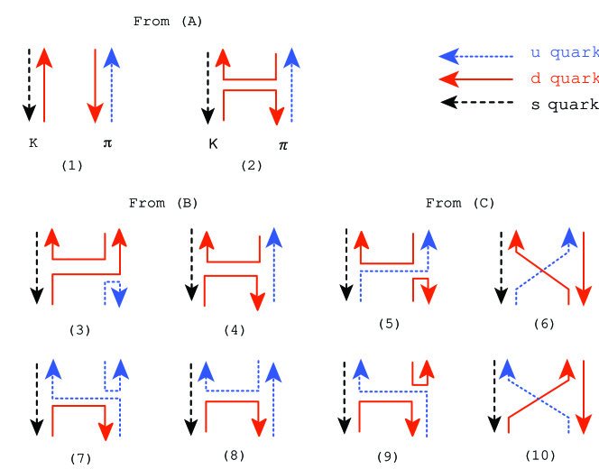
Figure 1: Quark propagators corresponding to Eq. $A1$-$A10$ in Appendix A.

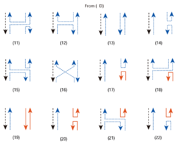
Figure 2: Quark propagators corresponding to Eqs. $A11$-$A22$ in Appendix A.

However, by assuming that $u$ and $d$ quarks have the same mass, we can categorize the 22 diagrams into six independent groups. Diagrams 1, 12, and 22 in Figs. 1 and 2 are compiled into Group 1. Similarly, diagrams 11, 17, 19 and 21 are compiled into Group 2, No. 2, 4, 8, and 13 in Group 3, No. 6, 10, and 15 in Group 4, diagrams 3, 5, 14, and 18 to Group 5, and diagrams 7, 9, 16, and 20 Group 6, respectively. According to Eq. (8) and Eqs. A1 - A22, the weights of each of these groups are given as follows:

Group 1: (14)

$${2\over 3}+{1\over 3}(-{1\over 2})(-1)+{1\over 3}(-{1\over 2})(-1)=1:A,$$

Group 2: (16)

$$({1\over 3})(-{1\over 2})+({1\over 3})(-{1\over 2})+({1\over 3})(-{1\over 2})(-1)+({1\over 3})(-{1\over 2})=0,$$

Group 3: (18)

$$({2\over 3})(-1)+(-{\sqrt{2}\over 3})(-{1\over\sqrt{2}})+(-{\sqrt{2}\over 3})(-{1\over\sqrt{2}})(-1)+({1\over 3})(-{1\over 2})=-{3\over 2}:H,$$

Group 4: (20)

$$(-{\sqrt{2}\over 3})(-{1\over\sqrt{2}})(+1)+(-{\sqrt{2}\over 3})({1\over\sqrt{2}})(-1)+({1\over 3})(-{1\over 2})={1\over 2}:X,$$

Group 5: (22)

$$(-{\sqrt{2}\over 3})(-{1\over\sqrt{2}})+(-{\sqrt{2}\over 3})({1\over\sqrt{2}})+({1\over 3})(-{1\over 2})(-1)(-1)+({1\over 3})(-{1\over 2})(-1)=0,$$

Group 6: (24)

$$(-{\sqrt{2}\over 3})(-{1\over\sqrt{2}})+(-{\sqrt{2}\over 3})({1\over\sqrt{2}})+({1\over 3})(-{1\over 2})(-1)+({1\over 3})(-{1\over 2})(-1)(-1)=0.$$

Here, $A$, $H$, and $X$ are denoting the type of the quark diagrams shown in Fig. 3. Finally, only the three diagrams shown in Fig. 3 remain to contribute to the $K\pi$ scattering amplitudes. Ultimately, both $I=3/2$ and $1/2$ channels can be expressed by using diagrams $A$, $H$, and $X$ as follows:

$$M(I=3/2) = A-X,$$ (26)

$$M(I=1/2) = A-{3\over 2}H+{1\over 2}X.$$ (27)

$A$, $H$, and $X$, are schematically shown in Fig. 3 and are given in terms of the quark propagators $G$ as

$$A(x_{1}{\large{}^{\prime}},x_{2}{\large{}^{\prime}},x_{1},x_{2}) = \mbox{Tr}\left(G(x_{1}{\large{}^{\prime}},x_{1})\gamma_{5}{G^{(s)}}(x_{1},x_{1}{\large{}^{\prime}})\gamma_{5}\right)\times\mbox{Tr}\left(G(x_{2}{\large{}^{\prime}},x_{2})\gamma_{5}G(x_{2},x_{2}{\large{}^{\prime}})\gamma_{5}\right)$$

$$= \mbox{Tr}\left(\gamma_{5}{G^{(s)}}(x_{1},x_{1}{\large{}^{\prime}})\gamma_{5}G(x_{1}{\large{}^{\prime}},x_{1})\right)\times\mbox{Tr}\left(\gamma_{5}G(x_{2},x_{2}{\large{}^{\prime}})\gamma_{5}G(x_{2}{\large{}^{\prime}},x_{2})\right),$$

$$H(x_{1}{\large{}^{\prime}},x_{2}{\large{}^{\prime}},x_{1},x_{2}) = \mbox{Tr}\left(G(x_{2}{\large{}^{\prime}},x_{2})\gamma_{5}G(x_{2},x_{1})\gamma_{5}{G^{(s)}}(x_{1},x_{1}{\large{}^{\prime}})\gamma_{5}G(x_{1}{\large{}^{\prime}},x_{2}{\large{}^{\prime}})\gamma_{5}\right)$$

$$= \mbox{Tr}\left(\gamma_{5}{G^{(s)}}(x_{1},x_{1}{\large{}^{\prime}})\gamma_{5}G(x_{1}{\large{}^{\prime}},x_{2}{\large{}^{\prime}})\gamma_{5}G(x_{2}{\large{}^{\prime}},x_{2})\gamma_{5}G(x_{2},x_{1})\right),$$

$$X(x_{1}{\large{}^{\prime}},x_{2}{\large{}^{\prime}},x_{1},x_{2}) = \mbox{Tr}\left(G(x_{1}{\large{}^{\prime}},x_{2})\gamma_{5}G(x_{2},x_{2}{\large{}^{\prime}})\gamma_{5}G(x_{2}{\large{}^{\prime}},x_{1})\gamma_{5}{G^{(s)}}(x_{1},x_{1}{\large{}^{\prime}})\gamma_{5}\right)$$ (28)

$$= \mbox{Tr}\left(\gamma_{5}{G^{(s)}}(x_{1},x_{1}{\large{}^{\prime}})\gamma_{5}G(x_{1}{\large{}^{\prime}},x_{2})\gamma_{5}G(x_{2},x_{2}{\large{}^{\prime}})\gamma_{5}G(x_{2}{\large{}^{\prime}},x_{1})\right).$$

Here, Tr stands for the trace over color and Dirac indices.

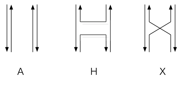
Figure 3: Diagrams $A$, $H$, and $X$.

II.3 Calculation of quark propagators using noise vectors

Now, we calculate the four-point functions in spatial momentum space using the Fourier transform of Eq. (28) at fixed $t$. In a standard lattice QCD simulation, quark propagators $G(=D^{-1})$ are calculated by inverting the quark matrix $D$,

$$D\vec{X}=\vec{B},$$ (29)

using a conjugate gradient type solver. While calculating the hadron four-point functions, we obtain the form

$$\sum_{\vec{x}}e^{i\vec{p}\vec{x}}\mbox{Tr}\left[D^{-1}(\vec{x},t;..)\cdots D^{-1}(..,\vec{x},t)\right].$$ (30)

For example, in the case of meson-meson scatterings composed of four quark lines, four quark propagators, $D^{-1}$, appear inside $\mbox{Tr}[\cdots]$ in Eq. (30).

If we calculate all necessary components of $D^{-1}$ with Eq. (29), a huge computational resource is required. In order to reduce the simulation cost, we introduce noise vectors

$$\sum_{j=1}^{N_{R}}\xi_{j}(\vec{x})^{\dagger}\xi_{j}(\vec{y})=\delta_{\vec{x},\vec{y}}$$ (31)

and rewrite Eq. (30) as

$$\frac{1}{N_{R}}\sum_{j}\sum_{\vec{x}}e^{i\vec{p}\vec{x}}\mbox{Tr}\left[\xi_{j}(\vec{x})^{\dagger}D^{-1}(\vec{x},t;..)\cdots D^{-1}(..,\vec{y},t)\xi_{j}(\vec{y})\right].$$ (32)

Then the four-point functions in the momentum space can be written as

$$A,\ \ X,\ \ H=\sum\vec{Y}^{\dagger}\vec{Z},$$ (33)

where

$$\vec{Y}\ \ \ \mbox{or}\ \ \ \vec{Z}=\cdots D^{-1}\cdots\xi.$$ (34)

Explicit formulas are given in Appendix B; We describe explicitly where the noise vectors are inserted.

In Eq.(30), not only $\vec{x}$ but also the color and Dirac indices are summed up because of Tr. Then one may extend Eq.(31) to include the color and Dirac degrees of freedom, which will reduce CPU time further. However, we do not take this in order to keep signal to noise ratio at reasonable levels.

III Numerical Results

The lattice simulations are carried out in the quenched approximation at $\beta=2.230$ on a $12^{3}\times 24$ lattice using an improved Iwasaki gauge action. Hopping parameters $\kappa_{ud}=0.1560$, $0.1580$, and $0.1600$ and $\kappa_{s}=0.1570$ are adopted for these simulations. The lattice spacing $a$ obtained using these parameters corresponds to 0.8144 GeV^-1.

Twenty different configurations separated by 2000 sweeps are used to evaluate the correlation functions $C_{\pi}$, $C_{K}$, and $C_{K\pi}$ at each $t$. We employ a complex $Z_{2}$ noise to represent the noise vectors in Eq. (31). The number of noise vectors in this equation is set to be four when the color and Dirac indices are fixed.

One could extend Eq. (31) to include the color and Dirac indices. In this case, the computational time is reduced significantly, but obtained results suffer from large errors. The choice here can be considered as a kind of dilution Foley05 .

Figure 4: $C_{\pi}$ and $C_{K}$ for $\kappa_{q}=0.156$, 0.158, and 0.160.

The obtained $C_{\pi}$ and $C_{K}$ are shown in Fig. 4. Both these correlations are well reproduced by one-pole fitted functions for $9\leq t\leq 12$,

$$C_{i}=Z_{i}\cosh(m_{i}(t-N_{t}/2)),$$ (35)

with $i$ being $K$ or $\pi$. The obtained parameters are shown in Table 1.

Table 1: Parameters for meson propagators

	$Z_{i}$	$m_{i}a$
$C_{\pi}$ ($\kappa_{q}=0.156$)	( 0.35369 $\pm$ 0.0002283 ) $\times 10^{-6}$	0.722183 $\pm$ 0.0004114
$C_{K}$ ($\kappa_{q}=0.156$)	( 0.457281 $\pm$ 0.0003214 ) $\times 10^{-6}$	0.701035 $\pm$ 0.0004315
$C_{\pi}$ ($\kappa_{q}=0.158$)	( 1.08796 $\pm$ 0.0008838 ) $\times 10^{-6}$	0.628463 $\pm$ 0.0004891
$C_{K}$ ($\kappa_{q}=0.158$)	( 0.803039 $\pm$ 0.0005946 ) $\times 10^{-6}$	0.653207 $\pm$ 0.0004654
$C_{\pi}$ ($\kappa_{q}=0.160$)	( 3.85386 $\pm$ 0.003642 ) $\times 10^{-6}$	0.526125 $\pm$ 0.0005567
$C_{K}$ ($\kappa_{q}=0.160$)	( 1.41634 $\pm$ 0.001258 ) $\times 10^{-6}$	0.606525 $\pm$ 0.0005159

III.1 Diagrams $A,H$, and $X$

As shown in Sec. II, only three different diagrams contribute to the correlation functions in the present system. Figure 5 shows the results obtained for diagrams $A$, $H$, and $X$ for $u$ and $d$ quarks of which hopping parameter, $\kappa_{q}=0.1580$. The $X$ and $H$ diagrams become negative at large $t$. At higher values of $\kappa_{q}=0.160$, the $H$ diagrams show similar behaviors. Since the contributions of $H$ and $X$ diagram distinguish $I=1/2$ from $I=3/2$, precise measurement of these contributions in large $t$ regions is important.

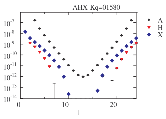
Figure 5: Numerical results for $A$, $H$, and $X$ contributions in the $K\pi$ four-point function at $\kappa_{q}=0.158$.

III.2 Lattice artifact

Because the lattice extent is finite, our $K\pi$ amplitude contaminated with the artifact shown in Fig. 6. These diagram contributions are large in meson correlator calculations at finite temperature in lattice QCD, and may mislead us as pointed out in Ref. Umeda07 . Such diagram are also seen in the current lattice QCD simulations of the two-meson state. This can be easily seen by evaluating the contribution of the fake diagrams in Fig. 6,

$$A_{\pi}e^{-m_{\pi}(N_{t}-t)}\times A_{K}e^{-m_{K}t}+A_{\pi}e^{-m_{\pi}t}\times A_{K}e^{-m_{K}(N_{t}-t)}$$

$$=2A_{\pi}A_{K}e^{-m_{\pi}N_{t}/2}e^{-m_{K}N_{t}/2}\cosh((m_{K}-m_{\pi})(t-N_{t}/2)).$$ (36)

When the mass difference between $\pi$ and $K$ is small, it acts as a constant mode and distorts the four-point function at large $t$. In Fig. 7, we show the above-mentioned contribution, Eq. (36), together with the numerical data corresponding to the four-point functions.

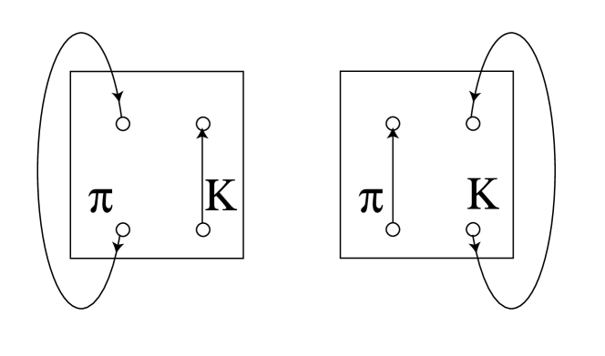
Figure 6: Diagrams that give rise to fake effects.

Another method of avoiding the above mentioned fake diagram is to impose a Dirichlet boundary conditions. But here we use a simpler method than it ; we subtract the contribution of these diagrams numerically from the obtained quantity. $A_{\pi}$, $A_{K}$, $m_{\pi}$, and $m_{K}$ in Eq. (20) can be evaluated from $\pi$ and $K$ propagator measurements. In the present case, we have the data corresponding to these two-point functions are sufficiently precise to allow subtractions of these effects, and hence, Eq. (36) can be subtracted from the $K\pi$ four-point data. In the following fitting processes, the $K\pi$ four-point data is used after the subtraction.

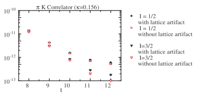
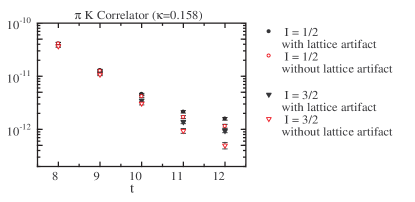
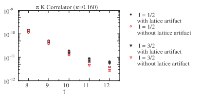
Figure 7: $K\pi$ four-point functions before and after subtracting the lattice artifact, Eq. (36). The figures from top to bottom correspond to $K_{q}$ values of 0.1560, 0.1580, and 0.1600, respectively. In each figure, for both $I=1/2$ and 3/2 channels, naive four-body correlations, $K\pi$, and those obtained after correction for the lattice artefact, Eq. (36), are shown.

III.3 Fitting analyses

In general, propagators $C_{i}$ are composed of many excited states of the same quantum number. If $t$ is sufficiently large $(1<<t<<N_{t})$ and the excited states have significantly higher masses than the ground-state mass, the contribution of the lowest energy state is predominant in the case of this propagator, and the one-pole model,

$$C_{i}(0,t)=Z_{1}\cosh(-m_{1}(t-N_{t}/2)),$$ (37)

fits the numerical data well. If there are contributions from higher states as well, a two-pole model,

$$C_{i}(0,t)=Z_{1}\cosh(-m_{1}(t-N_{t}/2))+Z_{2}\cosh(-m_{2}(t-N_{t}/2)),$$ (38)

would be more suitable than the one-pole model. Here, $m_{1}<m_{2}$, where $m_{1}$ is the lowest mass, and $m_{2}$ represents contributions from higher states. If the contribution from the higher states is very small, the fitting procedure for the two-pole model becomes unstable.

For $K$ and $\pi$ two-point functions, the one-pole ansatz, Eq.(37), works well, and hence,the masses of $K$ and $\pi$ are obtained with high accuracy (Fig. 4). The results of our simulation have already been shown in Table 1, and the values are consistent with those provided by CP-PACS.

For calculating the propagators of the $K\pi$ system (meson four-point function), we adopt a two-pole model by taking into account higher excited states; however, the calculation method in this case is not simple. A naive application of Eq. (38) is not stable when the fitting region we use is changed. In order to obtain reliable results, we take the steps as follows:

1. We apply Eq. (38) to $C_{K\pi}$ by changing the fitting region.

2. We choose a stable region, where the obtained $m_{1}$ shows a plateau, and calculate the average of $m_{1}$ in this region.

3. We also apply one-pole fitting and verify that $m_{1}$ obtained by two-pole fitting is lower than that obtained by one-pole fitting.

4. If the fitting procedure for the two-pole model is unstable, we adopt the results obtained with the one-pole model.

In the present simulation, $N_{t}$ is 24 and the source field is set at $t=0$. Because of its bosonic property, the propagator is symmetric at $t=N_{t}/2=12$. We apply the two-pole fit to propagator $C_{K\pi}$ in the region $t_{s}\leq t\leq N_{t}/2$. The larger $t_{s}$ corresponds to a propagator in the larger $t$ range, which is more reliable for picking up the ground state. However, in this case the number of available lattice points decreases. Figure 8 shows $m_{1}$ as a function of $t_{s}$. Then, we obtain the statistical average of the plots in Fig. 8 in order to obtain our final results, which are shown as horizontal lines in the figure.

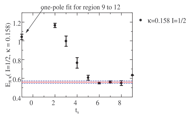
Figure 8: Effective mass extracted by one-pole and two-pole fittings as a function of $t_{S}$. $I=1/2$ and $\kappa=0.158$. The central region $(4\leq t_{s}\leq 8)$ is used to determine the ground-state energy. The value obtained and its error are shown by horizontal solid and dashed lines, respectively. The data point on the vertical axis shows the result obtained by the one-pole fit.

For $I=3/2$ with $\kappa=$ 0.1560 and 0.1580, two-pole fitting yields results with large statistical errors. Therefore, in these cases, we adopt one-pole fitting in the region $9\leq t\leq 12$. In the other cases, two-pole fitting gives better results than one-pole fitting, i.e., $m_{1}$ is smaller than the mass obtained with the one-pole model, and the statistical error is sufficiently small. The obtained values of $E_{K\pi}$ and $\Delta E=E_{K\pi}-(m_{\pi}+m_{K})$ at different values of the hopping parameter $\kappa$ are summarized in Table 2.

Table 2: Values obtained by fitting procedures for four-point function $C_{K\pi}$ and two-point functions $C_{K}$ and $C_{\pi}$. The $S$-wave scattering length $a_{0}$ is also calculated using these values.

	$\kappa_{ud}$	$E_{K\pi}$	$\delta E_{K\pi}$	$\Delta E$	$a_{0}$
	0.1560	0.6542	0.01804	-0.7690	0.4532
I = 1/2	0.1580	0.9264	0.01882	-0.3552	0.1598
	0.1600	1.066	0.008285	-0.0672	0.0222
	0.1560	1.379	0.02503	-0.0446	0.01850
I = 3/2	0.1580	1.258 a	0.03848	-0.0240	0.00896
	0.1600	1.087	0.002129	-0.0453	0.01505

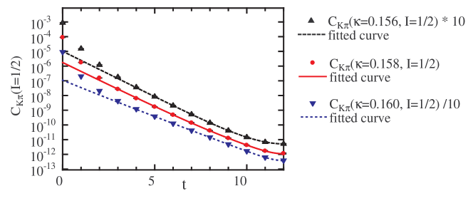
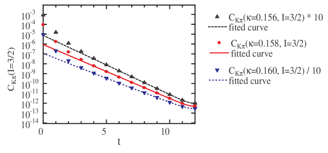
Figure 9: Four-body correlator (propagators of the $K\pi$ system ) and fitting curves for different $\kappa$ values. Upper and lower figures correspond to the $I=1/2$ and $I=3/2$ channels, respectively.

III.4 Chiral extrapolations and scattering length

In the present study, the pion masses $m_{\pi}$ are considerably larger than those determined experimentally, and hence, we need to adopt an extrapolation procedure. Although the behavior of $E_{K\pi}^{2}$ near the chiral limit is not very clear, we plot $E_{K\pi}^{2}$ for $I=1/2$ and 3/2 as a function of $1/\kappa$ in Fig. 10 together with $m_{\pi}^{2}$, and $m_{K}^{2}$; this is because $E_{K\pi}$ is expected to be dominated by $m_{\pi}$ and $m_{K}$.

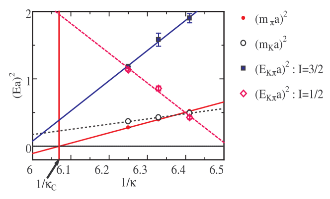
Figure 10: Chiral extrapolations of $m_{\pi}^{2}$, $m_{K}^{2}$, and $E_{K\pi}^{2}$. The horizontal axis is $1/\kappa_{q}$, where $\kappa_{q}$ is the hopping parameter for $u$ and $d$ quarks. The vertical line represents 1/$\kappa_{c}$ = 6.069351464.

The least mean square procedure for a linear function, $f(x)=ax+b$, provides us the errors for both $a$ and $b$. The least square procedure assumes that the fitted line passes through the center of the weight of plotted points. Therefore, errors of $a$ and $b$ are not independent but they are correlated; in the case that $a$ fluctuates positively $b$ must fluctuates negatively and vice versa. Hence, we may denote the line $y=ax+b$ as the middle line, $y=(a+\Delta a)x+(b-\Delta b)$ as the lower line and $y=(a-\Delta a)x+(b+\Delta b)$ as the upper line, with $\Delta a$ and $\Delta b$ being the error of $a$ and $b$, respectively. With these three lines, we evaluate the errors in the extrapolation process. Putting physical pion mass as $m_{\pi}=$ 139.57 MeV, the fitted line of $m_{\pi}^{2}$ provides us hopping parameter at physical point as $1/\kappa_{phys}$=$6.077724\pm 0.003071$. Here, the error, $\Delta(1/\kappa_{phys})$ = 0.003071, is one half of the difference between the value of the upper line and the one of the lower line at the physical pion mass. Also in the case of the energy of the two-particle state, we denote three curves as the middle, the upper and the lower which are the square root of the corresponding lines of the linear fit to the square of the energy of the two-particle state, respectively. The central value at physical points is determined by the middle curve and $1/\kappa_{phys}$. The error originates from the linear fitting, $\Delta_{1}$, is estimated from the difference between the upper curve and the lower curve at $1/\kappa_{phys}$. There exists another kind of the error, $\Delta_{2}$, which originates from $1/\kappa_{phys}$ which is evaluated from the difference of the middle curve at $1/\kappa_{phys}+\Delta(1/\kappa_{phys})$ and at $1/\kappa_{phys}-\Delta(1/\kappa_{phys})$. As a final error value, we may take root mean square of two independent errors, $\Delta_{1}$ and $\Delta_{2}$, as $\Delta E(\pi,K)=\sqrt{\Delta_{1}^{2}+\Delta_{2}^{2}}$. We also estimate errors of $E(\pi,K)$ in the other channel and $m_{K}$ in the same manner.

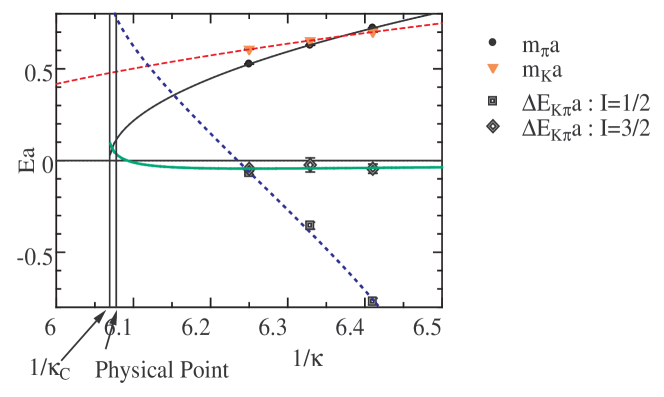
Figure 11: $\Delta E=E_{K\pi}-(m_{\pi}+m_{K})$ as a function of $1/\kappa_{q}$.

Substituting the obtained values into Lüscher’s formula, Eq. (2), we can obtain scattering length $a_{0}$. Unfortunately, the results obtained in the present study are limited to a fixed volume; nevertheless, by using the physical size of the lattice unit, we can evaluate $a_{0}$.

Let us rewrite Eq. (2) as

$$(E_{K\pi}-(m_{K}+m_{\pi}))\times\frac{m_{\pi}m_{K}L^{2}}{2\pi(m_{K}+m_{\pi})}=\Omega\left(\frac{a_{0}}{L}\right),\\$$ (39)

where

$$\Omega\left(\frac{a_{0}}{L}\right)=\frac{a_{0}}{L}\bigl{[}1+c_{1}{a_{0}\over L}+c_{2}({a_{0}\over L})^{2}\bigr{]}+O(L^{-6}).$$ (40)

The left-hand side of Eq. (39) represents the shift in energy caused by the interaction between $\pi$ and $K$; this energy shift can be evaluated from the correlations. The right-hand side, $\Omega\left(\frac{a_{0}}{L}\right)$, represents the effect of $a_{0}$ in the unit of box length. Figure 12 shows $\Omega$ as a function of $a_{0}/L$. $\Omega$ changes slowly at around ${a_{0}/L}\sim 0$, indicating that a small $a_{0}$ is sensitive to $\Delta E$ at around $\Delta E\sim 0$. Further, $a_{0}$ easily changes from a positive small value to a negative small value and vice versa.

The chiral extrapolation of $a_{0}$ is shown in Fig. 13. Our final results are summarized in Table 3. At all the calculation points, $a_{0}$ is positive, as shown in Table 2; however, the chiral extrapolation for $E_{K\pi}^{2}$ scaling leads to a change in the sign of $\Delta E$ and a subsequent change in the sign of $a_{0}$. At the physical point where $m_{\pi}=139.75$ MeV, $a_{0}(I=3/2)$ $m_{\pi}=-0.0837$ and $a_{0}(I=1/2)$ $m_{\pi}=-0.6248$. In both cases, $\Delta E>0$, the phase shift $\delta<0$, and forces are repulsive.

Table 3: $a_{0}$ at the physical point where $m_{\pi}$=139.75 MeV.

		$a_{0}$(MeV)		$a_{0}$ $m_{\pi}$
$I=1/2$		-0.8794 ${}^{+0.016}_{-0.017}$		-0.6248 ${}^{+0.0115}_{-0.0118}$
$I=3/2$		-0.1178 ${}^{+0.0712}_{-0.0901}$		-0.0837 ${}^{+0.0506}_{-0.0640}$

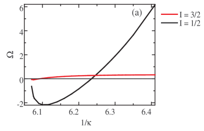
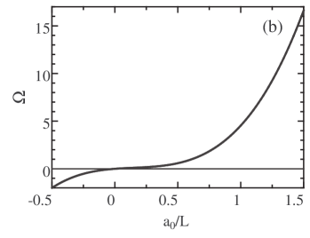
Figure 12: $\Omega$ evaluated through $\Delta E$ obtained by fitted curve in Fig. 11 (left-hand side) and $\Omega$ as a function of $a_{0}/L$ (right-hand side).

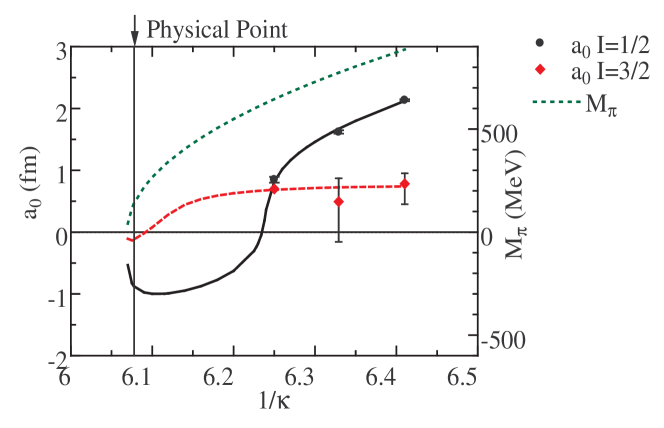
Figure 13: S-wave scattering length $a_{0}$ as a function of $1/\kappa_{q}$. Simulation data points at three values of $\kappa_{q}$ and extrapolated values at $m_{\pi}=140$ MeV.

IV Concluding Remarks

The scattering length, $a_{0}$ of the $I=3/2$ channel in $K\pi$ scattering has been studied by theoretical and experimental approaches so farJoh73 ; Mat74 ; Kar80 ; Ber91a ; Ber91b ; Bue03 ; Lla04 . Previous experiments have reported that $a_{3/2}m_{\pi}$ has a small negative value, i.e., $-0.13\sim-0.05$Joh73 ; Mat74 ; Kar80 . Small negative value was also claimed by a theoretical model based on the chiral perturbation theory as $a_{0}=-0.129\sim-0.05$Ber91a ; Ber91b ; Bue03 . The first lattice calculation of $K\pi$ scattering in the $I=3/2$ channel was performed by Miao et al.Mia04 , and the value of $a_{0}$ was found to be $-0.048$.

On the other hand, no direct simulations have been carried out on $K\pi$ scattering in the $I=1/2$ channel for estimations of $a_{0}$. The NPLQCD group carried out lattice simulations for $K\pi$ scattering in the $I=3/2$ channel and evaluated the $a_{0}$ values for both $I=3/2$ and $1/2$; the results of $I=1/2$ were obtained on the basis of chiral perturbations and not directly by simulations Bea06 . They obtained a small negative value of $-0.0574$ for the $I=3/2$ channel and found that $m_{\pi}a_{1/2}=+0.1725^{+0.0029}_{-0.0157}$ for the $I=1/2$ channel. The pion mass $m_{\pi}$ used by them was lower than that used in our present study. We could carry out a direct comparison of our results with those of NPLQCD group if we carry out our simulations at a low $m_{\pi}$. Flynn and NievesFly07 used the scalar form factors in semi-leptonic pseudo-scalar-to-pseudo-scalar decays to extract information on $K\pi$ scattering in the $I=1/2$ channel and obtained $m_{\pi}a_{1/2}$ = +0.179(17)(14).

In this paper, we presented a lattice QCD simulation of the $K\pi$ scattering length and formulas that make this calculation simple and feasible. We have observed the followings:

• $I=1/2$ and $3/2$ amplitudes can be expressed using quark diagrams, $A$, $H$ and $X$.

• use of a reasonable noise vector works well.

• a simple method for eliminating fake diagrams caused by the finite size of lattice is useful.

• the accurate measurements in large $t$ regions is important.

• the behavior of $\Delta E$ in the chiral extrapolation needs careful analysis.

Thus, it is now possible to study $K\pi$ scattering reactions on the basis of lattice QCD simulations. However, our present study does not provide adequate information on scalar mesons with the strangeness, i.e., $\kappa$, because our study is restricted to the zero-momentum case. Therefore, this paper does not include results on the phase shift $\delta(p)$, which is indicative of a $\kappa$ pole in the $K\pi$ channel. The study of $K\pi$ interactions is the first step in the study of hadron interactions including $s$-quarks, and we are now entering into the new era to study hyperon interaction from QCD.

We show exchanged mesons for meson-meson and nucleon-hyperon interactions in Table 4 and 5. $NN$ interactions include $\pi$ exchange and require lattices of very large size for estimation of the its large scattering length. On the contrary, $N\Lambda$ interactions can be studied using a lattice of reasonable size. Hence, $N\Lambda$ interactions are suitable for lattice studies because they have interaction ranges that can be fit to the Lüscher’s formula; these interactions will be extensively studied in future experiments in J-PARC and other laboratories.

Table 4: Exchanged pseudo-scalar mesons for baryon-baryon scatterings.

scattering system	exchanged mesons
$N-N$	$\pi$, $\eta$, $\eta^{\prime}$
$\Lambda-N$	$K$, $\eta$, $\eta^{\prime}$
$\Sigma-N$	$\pi$, $K$
$\Xi-N$	$\pi$, $\eta$, $\eta^{\prime}$

Table 5: Main contributions in $t/u$- and $s$-channels for pseudo-scalar meson-meson scattering.

scattering system	$t/u$-channel	$s$-channel
$\pi-\pi$	$\rho$, $\sigma$	$\rho$, $\sigma$
$K-\pi$	$\rho$, $\sigma$	$K^{*}$, $\kappa$

Appendix A $I=1/2$ $K\pi$ scattering amplitudes in terms of quark propagators

$$\langle O_{K^{0}}(x_{1}{\large{}^{\prime}})O_{\pi^{+}}(x_{2}{\large{}^{\prime}})O_{K^{0}}^{\dagger}(x_{1})O_{\pi^{+}}^{\dagger}(x_{2})\rangle$$ (41)

$$= {\rm Tr}\left(G^{(d)}(x_{2},x_{2}^{\prime})\gamma_{5}G^{(u)}(x_{2}^{\prime},x_{2})\gamma_{5}\right){\rm Tr}\left(G^{(d)}(x_{1}^{\prime},x_{1})\gamma_{5}G^{(s)}(x_{1},x_{1}^{\prime})\gamma_{5}\right)$$

$$- {\rm Tr}\left(G^{(d)}(x_{2},x_{1})\gamma_{5}G^{(s)}(x_{1},x_{1}^{\prime})\gamma_{5}G^{(d)}(x_{1}^{\prime},x_{2}^{\prime})\gamma_{5}G^{(u)}(x_{2}^{\prime},x_{2})\gamma_{5}\right)$$ (42)

$$\langle O_{K^{0}}(x_{1}{\large{}^{\prime}})O_{\pi^{+}}(x_{2}{\large{}^{\prime}})O_{K^{+}}^{\dagger}(x_{1})O_{\pi^{0}}^{\dagger}(x_{2})\rangle$$ (46)

$$= -\frac{1}{\sqrt{2}}{\rm Tr}\left(G^{(u)}(x_{2},x_{2})\gamma_{5}\right){\rm Tr}\left(G^{(u)}(x_{2}^{\prime},x_{1})\gamma_{5}G^{(s)}(x_{1},x_{1}^{\prime})\gamma_{5}G^{(d)}(x_{1}^{\prime},x_{2}^{\prime})\gamma_{5}\right)$$

$$+{1\over\sqrt{2}}{\rm Tr}\left(G^{(u)}(x_{2}^{\prime},x_{2})\gamma_{5}G^{(u)}(x_{2},x_{1})\gamma_{5}G^{(s)}(x_{1},x_{1}^{\prime})\gamma_{5}G^{(d)}(x_{1}^{\prime},x_{2}^{\prime})\gamma_{5}\right)$$

$$+\frac{1}{\sqrt{2}}{\rm Tr}\left(G^{(d)}(x_{2},x_{2})\gamma_{5}\right){\rm Tr}\left(G^{(s)}(x_{1},x_{1}^{\prime})\gamma_{5}G^{(d)}(x_{1}^{\prime},x_{2}^{\prime})\gamma_{5}G^{(u)}(x_{2}^{\prime},x_{1})\gamma_{5}\right)$$

$$-\frac{1}{\sqrt{2}}{\rm Tr}\left(G^{(d)}(x_{1}^{\prime},x_{2})\gamma_{5}G^{(d)}(x_{2},x_{2}^{\prime})\gamma_{5}G^{(u)}(x_{2}^{\prime},x_{1})\gamma_{5}G^{(s)}(x_{1},x_{1}^{\prime})\gamma_{5}\right)$$

$$\langle O_{K^{+}}(x_{1}{\large{}^{\prime}})O_{\pi^{0}}(x_{2}{\large{}^{\prime}})O_{K^{0}}^{\dagger}(x_{1})O_{\pi^{+}}^{\dagger}(x_{2})\rangle$$ (50)

$$= -\frac{1}{\sqrt{2}}{\rm Tr}\left(G^{(u)}(x_{2}^{\prime},x_{2}^{\prime})\gamma_{5}\right){\rm Tr}\left(G^{(u)}(x_{1}^{\prime},x_{2})\gamma_{5}G^{(d)}(x_{2},x_{1})\gamma_{5}G^{(s)}(x_{1},x_{1}^{\prime})\gamma_{5}\right)$$

$$+\frac{1}{\sqrt{2}}{\rm Tr}\left(G^{(u)}(x_{2}^{\prime},x_{2})\gamma_{5}G^{(d)}(x_{2},x_{1})\gamma_{5}G^{(s)}(x_{1},x_{1}^{\prime})\gamma_{5}G^{(u)}(x_{1}^{\prime},x_{2}^{\prime})\gamma_{5}\right)$$

$$+\frac{1}{\sqrt{2}}{\rm Tr}\left(G^{(d)}(x_{2}^{\prime},x_{2}^{\prime})\gamma_{5}\right){\rm Tr}\left(G^{(d)}(x_{2},x_{1})\gamma_{5}G^{(s)}(x_{1},x_{1}^{\prime})\gamma_{5}G^{(u)}(x_{1}^{\prime},x_{2})\gamma_{5}\right)$$

$$-\frac{1}{\sqrt{2}}{\rm Tr}\left(G^{(d)}(x_{2}^{\prime},x_{1})\gamma_{5}G^{(s)}(x_{1},x_{1^{\prime}})\gamma_{5}G^{(u)}(x_{1}^{\prime},x_{2})\gamma_{5}G^{(d)}(x_{2},x_{2}^{\prime})\gamma_{5}\right)$$

$$\langle O_{K^{+}}(x_{1}{\large{}^{\prime}})O_{\pi^{0}}(x_{2}{\large{}^{\prime}})O_{K^{+}}^{\dagger}(x_{1})O_{\pi^{0}}^{\dagger}(x_{2})\rangle$$ (56)

$$= -\frac{1}{2}{\rm Tr}\left(G^{(u)}(x_{2}^{\prime},x_{2}^{\prime})\gamma_{5}\right){\rm Tr}\left(G^{(u)}(x_{2},x_{2})\gamma_{5}\right){\rm Tr}\left(G^{(d)}(x_{1}^{\prime},x_{1})\gamma_{5}G^{(s)}(x_{1},x_{1}^{\prime})\gamma_{5}\right)$$

$$+\frac{1}{2}{\rm Tr}\left(G^{(u)}(x_{1}^{\prime},x_{1})\gamma_{5}G^{(s)}(x_{1},x_{1}^{\prime})\gamma_{5}\right){\rm Tr}\left(G^{(u)}(x_{2}^{\prime},x_{2})\gamma_{5}G^{(u)}(x_{2},x_{2}^{\prime})\gamma_{5}\right)$$

$$-\frac{1}{2}{\rm Tr}\left(G^{(u)}(x_{1}^{\prime},x_{2}^{\prime})\gamma_{5}G^{(u)}(x_{2}^{\prime},x_{2})\gamma_{5}G^{(u)}(x_{2},x_{1})\gamma_{5}G^{(s)}(x_{1},x_{1}^{\prime})\gamma_{5}\right)$$

$$+\frac{1}{2}{\rm Tr}\left(G^{(u)}(x_{1}^{\prime},x_{2}^{\prime})\gamma_{5}G^{(u)}(x_{2}^{\prime},x_{1})\gamma_{5}G^{(s)}(x_{1},x_{1}^{\prime})\gamma_{5}\right){\rm Tr}\left(G^{(u)}(x_{2},x_{2})\gamma_{5}\right)$$

$$-\frac{1}{2}{\rm Tr}\left(G^{(u)}(x_{1}^{\prime},x_{2})\gamma_{5}G^{(u)}(x_{2},x_{2}^{\prime})\gamma_{5}G^{(u)}(x_{2}^{\prime},x_{1})\gamma_{5}G^{(s)}(x_{1},x_{1}^{\prime})\gamma_{5}\right)$$

$$+\frac{1}{2}{\rm Tr}\left(G^{(u)}(x_{1}^{\prime},x_{2})\gamma_{5}G^{(u)}(x_{2},x_{1})\gamma_{5}G^{(s)}(x_{1},x_{1}^{\prime})\gamma_{5}\right){\rm Tr}\left(G^{(u)}(x_{2}^{\prime},x_{2}^{\prime})\gamma_{5}\right)$$

$$+ \frac{1}{2}{\rm Tr}\left(G^{(u)}(x_{1}^{\prime},x_{1})\gamma_{5}G^{(s)}(x_{1},x_{1}^{\prime})\gamma_{5}\right){\rm Tr}\left(G^{(u)}(x_{2}^{\prime},x_{2}^{\prime})\gamma_{5}\right){\rm Tr}\left(G^{(d)}(x_{2},x_{2})\gamma_{5}\right)$$ (62)

$$-\frac{1}{2}{\rm Tr}\left(G^{(u)}(x_{1}^{\prime},x_{2}^{\prime})\gamma_{5}G^{(u)}(x_{2}^{\prime},x_{1})\gamma_{5}G^{(s)}(x_{1},x_{1}^{\prime})\gamma_{5}\right){\rm Tr}\left(G^{(d)}(x_{2},x_{2})\gamma_{5}\right)$$

$$+\frac{1}{2}{\rm Tr}\left(G^{(u)}(x_{1}^{\prime},x_{1})\gamma_{5}G^{(s)}(x_{1},x_{1}^{\prime})\gamma_{5}\right){\rm Tr}\left(G^{(u)}(x_{2},x_{2})\gamma_{5}\right){\rm Tr}\left(G^{(d)}(x_{2}^{\prime},x_{2}^{\prime})\gamma_{5}\right)$$

$$-\frac{1}{2}{\rm Tr}\left(G^{(u)}(x_{1}^{\prime},x_{2})\gamma_{5}G^{(u)}(x_{2},x_{1})\gamma_{5}G^{(s)}(x_{1},x_{1}^{\prime})\gamma_{5}\right){\rm Tr}\left(G^{(d)}(x_{2}^{\prime},x_{2}^{\prime})\gamma_{5}\right)$$

$$-\frac{1}{2}{\rm Tr}\left(G^{(d)}(x_{2}^{\prime},x_{2}^{\prime})\gamma_{5}\right){\rm Tr}\left(G^{(d)}(x_{2},x_{2})\gamma_{5}\right){\rm Tr}\left(G^{(s)}(x_{1},x_{1}^{\prime})\gamma_{5}G^{(u)}(x_{1}^{\prime},x_{1})\gamma_{5}\right)$$

$$+\frac{1}{2}{\rm Tr}\left(G^{(d)}(x_{2}^{\prime},x_{2})\gamma_{5}G^{(d)}(x_{2},x_{2}^{\prime})\gamma_{5}\right){\rm Tr}\left(G^{(s)}(x_{1},x_{1}^{\prime})\gamma_{5}G^{(u)}(x_{1}^{\prime},x_{1})\gamma_{5}\right)$$

Appendix B Explicit forms of the diagram $A$, $H$ and $X$

In this section, we employ two independent random noises, $\xi$ and $\eta$. They are a function of the spatial coordinate, i.e., they live on a each time slice.

$$\frac{1}{N_{R}}\sum_{j}\quad\xi_{j}(\vec{x})^{\dagger}\xi_{j}(\vec{y}) = \delta_{\vec{x},\vec{y}}$$ (63)

$$\frac{1}{N_{R}}\sum_{j}\quad\eta_{j}(\vec{x})^{\dagger}\eta_{j}(\vec{y}) = \delta_{\vec{x},\vec{y}}$$ (64)

B.1 Diagram A

$$A (\vec{p}_{n},-\vec{p}_{n},\vec{p}_{m},-\vec{p}_{m})$$ (65)

$$= \sum_{\vec{x}_{1}{\large{}^{\prime}}}\sum_{\vec{x}_{2}{\large{}^{\prime}}}\sum_{\vec{x}_{1}}\sum_{\vec{x}_{2}}\frac{e^{+i\vec{p}_{n}\cdot\vec{x}_{1}{\large{}^{\prime}}}}{L^{3}}\frac{e^{-i\vec{p}_{n}\cdot\vec{x}_{2}{\large{}^{\prime}}}}{L^{3}}\frac{e^{+i\vec{p}_{m}\cdot\vec{x}_{1}}}{L^{3}}\frac{e^{-i\vec{p}_{m}\cdot\vec{x}_{2}}}{L^{3}}$$ (66)

$$\times A((\vec{x}_{1}{\large{}^{\prime}},t),(\vec{x}_{2}{\large{}^{\prime}},t),(\vec{x}_{1},t_{S}),(\vec{x}_{2},t_{S}))$$ (67)

$$= \sum_{\vec{x}_{1}{\large{}^{\prime}}}\sum_{\vec{x}_{1}}\frac{e^{+i\vec{p}_{n}\cdot\vec{x}_{1}{\large{}^{\prime}}}}{L^{3}}\frac{e^{+i\vec{p}_{m}\cdot\vec{x}_{1}}}{L^{3}}$$ (68)

$$\times \mbox{Tr}\left(\gamma_{5}{G^{(s)}}(\vec{x}_{1},t_{S};\vec{x}_{1}{\large{}^{\prime}},t)\gamma_{5}G(\vec{x}_{1}{\large{}^{\prime}},t;\vec{x}_{1},t_{S})\right)$$ (69)

$$\times \sum_{\vec{x}_{2}{\large{}^{\prime}}}\sum_{\vec{x}_{2}}\frac{e^{-i\vec{p}_{n}\cdot\vec{x}_{2}{\large{}^{\prime}}}}{L^{3}}\frac{e^{-i\vec{p}_{m}\cdot\vec{x}_{2}}}{L^{3}}$$ (70)

$$\times \mbox{Tr}\left(\gamma_{5}G(\vec{x}_{2},t_{S};\vec{x}_{2}{\large{}^{\prime}},t)\gamma_{5}G(\vec{x}_{2}{\large{}^{\prime}},t;\vec{x}_{2},t_{S})\right)$$ (71)

$$= \frac{1}{N_{R}}\sum_{j_{1}}\quad\sum_{\vec{y}_{1}}\sum_{\vec{x}_{1}{\large{}^{\prime}}}\sum_{\vec{x}_{1}}\frac{e^{+i\vec{p}_{n}\cdot\vec{x}_{1}{\large{}^{\prime}}}}{L^{3}}\frac{e^{+i\vec{p}_{m}\cdot\vec{x}_{1}}}{L^{3}}$$ (72)

$$\times \mbox{Tr}\left(\xi_{j_{1}}^{\dagger}(\vec{y}_{1})\gamma_{5}{G^{(s)}}(\vec{y}_{1},t_{S};\vec{x}_{1}{\large{}^{\prime}},t)\gamma_{5}G(\vec{x}_{1}{\large{}^{\prime}},t;\vec{x}_{1},t_{S})\xi_{j_{1}}(\vec{x}_{1})\right)$$ (73)

$$\times \frac{1}{N_{R}}\sum_{j_{2}}\quad\sum_{\vec{y}_{2}}\sum_{\vec{x}_{2}{\large{}^{\prime}}}\sum_{\vec{x}_{2}}\frac{e^{-i\vec{p}_{n}\cdot\vec{x}_{2}{\large{}^{\prime}}}}{L^{3}}\frac{e^{-i\vec{p}_{m}\cdot\vec{x}_{2}}}{L^{3}}$$ (74)

$$\times \mbox{Tr}\left(\eta_{j_{2}}^{\dagger}(\vec{y}_{2})\gamma_{5}G(\vec{y}_{2},t_{S};\vec{x}_{2}{\large{}^{\prime}},t)\gamma_{5}G(\vec{x}_{2}{\large{}^{\prime}},t;\vec{x}_{2},t_{S})\eta_{j_{2}}(\vec{x}_{2})\right)$$ (75)

We can write the trace terms as

$$\mbox{Tr}\left(\gamma_{5}{G^{(s)}}(\vec{x}_{1},t_{S};\vec{x}_{1}{\large{}^{\prime}},t)\gamma_{5}G(\vec{x}_{1}{\large{}^{\prime}},t;\vec{x}_{1},t_{S})\right)=\sum_{a,\alpha}\langle a,\alpha|\gamma_{5}{G^{(s)}}(\vec{x}_{1},t_{S};\vec{x}_{1}{\large{}^{\prime}},t)\gamma_{5}G(\vec{x}_{1}{\large{}^{\prime}},t;\vec{x}_{1},t_{S})|a,\alpha\rangle$$ (76)

$$\mbox{Tr}\left(\gamma_{5}G(\vec{x}_{2},t_{S};\vec{x}_{2}{\large{}^{\prime}},t)\gamma_{5}G(\vec{x}_{2}{\large{}^{\prime}},t;\vec{x}_{2},t_{S})\right)=\sum_{a,\alpha}\langle a,\alpha|\gamma_{5}G(\vec{x}_{2},t_{S};\vec{x}_{2}{\large{}^{\prime}},t)\gamma_{5}G(\vec{x}_{2}{\large{}^{\prime}},t;\vec{x}_{2},t_{S})|a,\alpha\rangle$$ (77)

where $a$ and $\alpha$ stand for the color and Dirac indices, respectively.

Then

$$A(\vec{p}_{n},-\vec{p}_{n},\vec{p}_{m},-\vec{p}_{m};t,t_{S})=\frac{1}{N_{R}}\sum_{j_{1}}\quad\sum_{a,\alpha}\sum_{\vec{x}_{1}{\large{}^{\prime}}}\vec{Z}_{1}(\vec{x}_{1}{\large{}^{\prime}},t;t_{S})^{\dagger}\frac{e^{+i\vec{p}_{n}\cdot\vec{x}_{1}{\large{}^{\prime}}}}{L^{3}}\vec{Y}_{1}(\vec{x}_{1}{\large{}^{\prime}},t;t_{S})$$

$$\times\frac{1}{N_{R}}\sum_{j_{2}}\quad\sum_{a,\alpha}\sum_{\vec{x}_{2}{\large{}^{\prime}}}\vec{Z}_{2}(\vec{x}_{2}{\large{}^{\prime}},t;t_{S})^{\dagger}\frac{e^{-i\vec{p}_{n}\cdot\vec{x}_{2}{\large{}^{\prime}}}}{L^{3}}\vec{Y}_{2}(\vec{x}_{2}{\large{}^{\prime}},t;t_{S})$$ (78)

where

$$\vec{Y}_{1} \equiv G\frac{e^{+i\vec{p}_{m}\cdot\vec{x}_{1}}}{L^{3}}\xi_{j_{1}}|a,\alpha\rangle\quad\mbox{or}$$ (79)

$$\vec{Y}_{1}(\vec{x}_{1}{\large{}^{\prime}},t;t_{S}) = \sum_{\vec{x}_{1}}G(\vec{x}_{1}{\large{}^{\prime}},t;\vec{x}_{1},t_{S})\frac{e^{+i\vec{p}_{m}\cdot\vec{x}_{1}}}{L^{3}}\xi_{j_{1}}(\vec{x}_{1})|a,\alpha\rangle$$ (80)

$$\vec{Z}_{1} \equiv \gamma_{5}{G^{(s)}}^{\dagger}\gamma_{5}\xi_{j_{1}}|a,\alpha\rangle\quad\mbox{or}$$ (81)

$$\vec{Z}_{1}(\vec{x}_{1}{\large{}^{\prime}},t;t_{S}) = \sum_{\vec{y}_{1}}\gamma_{5}{G^{(s)}}^{\dagger}(\vec{x}_{1}{\large{}^{\prime}},t;\vec{y}_{1},t_{S})\gamma_{5}\xi_{j_{1}}(\vec{y}_{1})|a,\alpha\rangle$$ (82)

$$\vec{Y}_{2} \equiv G\frac{e^{-i\vec{p}_{m}\cdot\vec{x}_{2}}}{L^{3}}\eta_{j_{2}}|a,\alpha\rangle\quad\mbox{or}$$ (83)

$$\vec{Y}_{2}(\vec{x}_{2}{\large{}^{\prime}},t;t_{S}) = \sum_{\vec{x}_{2}}G(\vec{x}_{2}{\large{}^{\prime}},t;\vec{x}_{2},t_{S})\frac{e^{-i\vec{p}_{m}\cdot\vec{x}_{2}}}{L^{3}}\eta_{j_{2}}(\vec{x}_{2})|a,\alpha\rangle$$ (84)

$$\vec{Z}_{2} \equiv \gamma_{5}G^{\dagger}\gamma_{5}\eta_{j_{2}}|a,\alpha\rangle\quad\mbox{or}$$ (85)

$$\vec{Z}_{2}(\vec{x}_{2}{\large{}^{\prime}},t;t_{S}) = \sum_{\vec{y}_{2}}\gamma_{5}G^{\dagger}(\vec{x}_{2}{\large{}^{\prime}},t;\vec{y}_{2},t_{S})\gamma_{5}\eta_{j_{2}}(\vec{y}_{2})|a,\alpha\rangle$$ (86)

where $\dagger$ or Hermite conjugate includes the color, Dirac and site indices.

Indices of these vectors are

$$Y^{b}_{\beta}(\vec{x}^{\prime},t;t_{S})=\sum_{\vec{x}}\sum_{c,\gamma}G^{b,c}_{\beta,\gamma}(\vec{x}^{\prime},t;\vec{x},t_{S})\xi(\vec{x})|a,\alpha\rangle_{c,\gamma}$$ (87)

$$Z^{b}_{\beta}(\vec{x}^{\prime},t;t_{S})=\sum_{\vec{x}}\sum_{c,\gamma}\left(G^{c,b}_{\gamma,\beta}(\vec{x},t_{S};\vec{x}^{\prime},t)\right)^{*}\xi(\vec{x})|a,\alpha\rangle_{c,\gamma}$$ (88)

$$\vec{Z}^{\dagger}\cdot\vec{Y}=\sum_{b}\sum_{\beta}\sum_{\vec{x}^{\prime}}\left(Z^{b}_{\beta}(\vec{x}^{\prime},t;t_{S})\right)^{*}Y^{b}_{\beta}(\vec{x}^{\prime},t;t_{S})$$ (89)

B.2 Diagram H

$$H (\vec{p}_{n},-\vec{p}_{n},\vec{p}_{m},-\vec{p}_{m})$$ (90)

$$= \sum_{\vec{x}_{1}{\large{}^{\prime}}}\sum_{\vec{x}_{2}{\large{}^{\prime}}}\sum_{\vec{x}_{1}}\sum_{\vec{x}_{2}}\frac{e^{+i\vec{p}_{n}\cdot\vec{x}_{1}{\large{}^{\prime}}}}{L^{3}}\frac{e^{-i\vec{p}_{n}\cdot\vec{x}_{2}{\large{}^{\prime}}}}{L^{3}}\frac{e^{+i\vec{p}_{m}\cdot\vec{x}_{1}}}{L^{3}}\frac{e^{-i\vec{p}_{m}\cdot\vec{x}_{2}}}{L^{3}}$$

$$\times H((\vec{x}_{1}{\large{}^{\prime}},t),(\vec{x}_{2}{\large{}^{\prime}},t),(\vec{x}_{1},t_{S}),(\vec{x}_{2},t_{S}))$$

$$= \sum_{\vec{x}_{1}{\large{}^{\prime}}}\sum_{\vec{x}_{2}{\large{}^{\prime}}}\sum_{\vec{x}_{1}}\sum_{\vec{x}_{2}}\frac{e^{+i\vec{p}_{n}\cdot\vec{x}_{1}{\large{}^{\prime}}}}{L^{3}}\frac{e^{-i\vec{p}_{n}\cdot\vec{x}_{2}{\large{}^{\prime}}}}{L^{3}}\frac{e^{+i\vec{p}_{m}\cdot\vec{x}_{1}}}{L^{3}}\frac{e^{-i\vec{p}_{m}\cdot\vec{x}_{2}}}{L^{3}}$$

$$\times \mbox{Tr}\left(\gamma_{5}{G^{(s)}}(\vec{x}_{1},t_{S};\vec{x}_{1}{\large{}^{\prime}},t)\gamma_{5}G(\vec{x}_{1}{\large{}^{\prime}},t;\vec{x}_{2}{\large{}^{\prime}},t)\gamma_{5}G(\vec{x}_{2}{\large{}^{\prime}},t;\vec{x}_{2},t_{S})\gamma_{5}G(\vec{x}_{2},t_{S};\vec{x}_{1},t_{S})\right)$$

$$= \frac{1}{N_{R}}\sum_{j}\quad\sum_{\vec{y}_{1}}\sum_{\vec{x}_{1}{\large{}^{\prime}}}\sum_{\vec{x}_{2}{\large{}^{\prime}}}\sum_{\vec{x}_{1}}\sum_{\vec{x}_{2}}\frac{e^{+i\vec{p}_{n}\cdot\vec{x}_{1}{\large{}^{\prime}}}}{L^{3}}\frac{e^{-i\vec{p}_{n}\cdot\vec{x}_{2}{\large{}^{\prime}}}}{L^{3}}\frac{e^{+i\vec{p}_{m}\cdot\vec{x}_{1}}}{L^{3}}\frac{e^{-i\vec{p}_{m}\cdot\vec{x}_{2}}}{L^{3}}$$

$$\times \mbox{Tr}\left(\xi_{j}^{\dagger}(\vec{y}_{1})\gamma_{5}{G^{(s)}}(\vec{y}_{1},t_{S};\vec{x}_{1}{\large{}^{\prime}},t)\gamma_{5}G(\vec{x}_{1}{\large{}^{\prime}},t;\vec{x}_{2}{\large{}^{\prime}},t)\right.$$

$$\times \left.\gamma_{5}G(\vec{x}_{2}{\large{}^{\prime}},t;\vec{x}_{2},t_{S})\gamma_{5}G(\vec{x}_{2},t_{S};\vec{x}_{1},t_{S})\xi_{j}(\vec{x}_{1})\right)$$

We can write a trace term as

$$\mbox{Tr}\left(\gamma_{5}{G^{(s)}}(\vec{x}_{1},t_{S};\vec{x}_{1}{\large{}^{\prime}},t)\gamma_{5}G(\vec{x}_{1}{\large{}^{\prime}},t;\vec{x}_{2}{\large{}^{\prime}},t)\gamma_{5}G(\vec{x}_{2}{\large{}^{\prime}},t;\vec{x}_{2},t_{S})\gamma_{5}G(\vec{x}_{2},t_{S};\vec{x}_{1},t_{S})\right)$$

$$=\sum_{a,\alpha}\langle a,\alpha|\gamma_{5}{G^{(s)}}(\vec{x}_{1},t_{S};\vec{x}_{1}{\large{}^{\prime}},t)\gamma_{5}G(\vec{x}_{1}{\large{}^{\prime}},t;\vec{x}_{2}{\large{}^{\prime}},t)\gamma_{5}G(\vec{x}_{2}{\large{}^{\prime}},t;\vec{x}_{2},t_{S})\gamma_{5}G(\vec{x}_{2},t_{S};\vec{x}_{1},t_{S})|a,\alpha\rangle$$ (91)

Then

$$H(\vec{p}_{n},-\vec{p}_{n},\vec{p}_{m},-\vec{p}_{m};t,t_{S})=\frac{1}{N_{R}}\sum_{j}\quad\sum_{\vec{x}_{2}{\large{}^{\prime}}}\vec{Z}^{\dagger}(\vec{x}_{2}{\large{}^{\prime}},t;t_{S})\frac{e^{-i\vec{p}_{n}\cdot\vec{x}_{2}{\large{}^{\prime}}}}{L^{3}}\vec{Y}(\vec{x}_{2}{\large{}^{\prime}},t;t_{S})$$ (92)

where

$$\vec{Y} \equiv \sum_{\vec{x}_{2}}\sum_{\vec{x}_{1}}G\frac{e^{-i\vec{p}_{m}\cdot\vec{x}_{2}}}{L^{3}}\gamma_{5}G\frac{e^{+i\vec{p}_{m}\cdot\vec{x}_{1}}}{L^{3}}\xi_{j}|a,\alpha\rangle\quad\mbox{or}$$ (93)

$$\vec{Y}(\vec{x}_{2}{\large{}^{\prime}},t;t_{S}) = \sum_{\vec{x}_{2}}\sum_{\vec{x}_{1}}G(\vec{x}_{2}{\large{}^{\prime}},t;\vec{x}_{2},t_{S})\frac{e^{-i\vec{p}_{m}\cdot\vec{x}_{2}}}{L^{3}}\gamma_{5}G(\vec{x}_{2},t_{S};\vec{x}_{1},t_{S})\frac{e^{+i\vec{p}_{m}\cdot\vec{x}_{1}}}{L^{3}}$$ (94)

$$\times \xi_{j}(\vec{x}_{1})|a,\alpha\rangle$$

$$= \sum_{\vec{x}_{2}}G(\vec{x}_{2}{\large{}^{\prime}},t;\vec{x}_{2},t_{S})\gamma_{5}\frac{e^{-i\vec{p}_{m}\cdot\vec{x}_{2}}}{L^{3}}\vec{Y}_{1}(\vec{x}_{2},t_{S};t_{S})$$

Here

$$\vec{Y}_{1}(\vec{x}_{2},t_{S};t_{S})\equiv\sum_{\vec{x}_{1}}G(\vec{x}_{2},t_{S};\vec{x}_{1},t_{S})\frac{e^{+i\vec{p}_{m}\cdot\vec{x}_{1}}}{L^{3}}\xi_{j}(\vec{x}_{1})|a,\alpha\rangle$$ (95)

$$\vec{Z} \equiv \sum_{\vec{x}_{1}{\large{}^{\prime}}}\gamma_{5}G^{\dagger}\frac{e^{-i\vec{p}_{n}\cdot\vec{x}_{1}{\large{}^{\prime}}}}{L^{3}}\gamma_{5}{G^{(s)}}^{\dagger}\gamma_{5}\xi_{j}|a,\alpha\rangle\quad\mbox{or}$$ (96)

$$\vec{Z}(\vec{x}_{2}{\large{}^{\prime}},t;t_{S}) = \sum_{\vec{x}_{1}{\large{}^{\prime}}}\gamma_{5}G^{\dagger}(\vec{x}_{2}{\large{}^{\prime}},t;\vec{x}_{1}{\large{}^{\prime}},t)\frac{e^{-i\vec{p}_{n}\cdot\vec{x}_{1}{\large{}^{\prime}}}}{L^{3}}\sum_{\vec{y}_{1}}\gamma_{5}{G^{(s)}}^{\dagger}(\vec{x}_{1}{\large{}^{\prime}},t;\vec{y}_{1},t_{S})\gamma_{5}$$ (97)

$$\times \xi_{j}(\vec{y}_{1})|a,\alpha\rangle$$ (98)

$$= \sum_{\vec{x}_{1}{\large{}^{\prime}}}\gamma_{5}G^{\dagger}(\vec{x}_{2}{\large{}^{\prime}},t;\vec{x}_{1}{\large{}^{\prime}},t)\frac{e^{-i\vec{p}_{n}\cdot\vec{x}_{1}{\large{}^{\prime}}}}{L^{3}}\vec{Z}_{1}(\vec{x}_{1}{\large{}^{\prime}},t;t_{S})$$ (99)

Here

$$\vec{Z}_{1}(\vec{x}_{1}{\large{}^{\prime}},t;t_{S})\equiv\sum_{\vec{y}_{1}}\gamma_{5}{G^{(s)}}^{\dagger}(\vec{x}_{1}{\large{}^{\prime}},t;\vec{y}_{1},t_{S})\gamma_{5}\xi_{j}(\vec{y}_{1})|a,\alpha\rangle$$ (100)

B.3 Diagram X

$$X (\vec{p}_{n},-\vec{p}_{n},\vec{p}_{m},-\vec{p}_{m})$$ (101)

$$= \sum_{\vec{x}_{1}{\large{}^{\prime}}}\sum_{\vec{x}_{2}{\large{}^{\prime}}}\sum_{\vec{x}_{1}}\sum_{\vec{x}_{2}}\frac{e^{+i\vec{p}_{n}\cdot\vec{x}_{1}{\large{}^{\prime}}}}{L^{3}}\frac{e^{-i\vec{p}_{n}\cdot\vec{x}_{2}{\large{}^{\prime}}}}{L^{3}}\frac{e^{+i\vec{p}_{m}\cdot\vec{x}_{1}}}{L^{3}}\frac{e^{-i\vec{p}_{m}\cdot\vec{x}_{2}}}{L^{3}}$$

$$\times X((\vec{x}_{1}{\large{}^{\prime}},t),(\vec{x}_{2}{\large{}^{\prime}},t),(\vec{x}_{1},t_{S}),(\vec{x}_{2},t_{S}))$$

$$= \sum_{\vec{x}_{1}{\large{}^{\prime}}}\sum_{\vec{x}_{2}{\large{}^{\prime}}}\sum_{\vec{x}_{1}}\sum_{\vec{x}_{2}}\frac{e^{+i\vec{p}_{n}\cdot\vec{x}_{1}{\large{}^{\prime}}}}{L^{3}}\frac{e^{-i\vec{p}_{n}\cdot\vec{x}_{2}{\large{}^{\prime}}}}{L^{3}}\frac{e^{+i\vec{p}_{m}\cdot\vec{x}_{1}}}{L^{3}}\frac{e^{-i\vec{p}_{m}\cdot\vec{x}_{2}}}{L^{3}}$$

$$\times \mbox{Tr}\left(\gamma_{5}{G^{(s)}}(\vec{x}_{1},t_{S};\vec{x}_{1}{\large{}^{\prime}},t)\gamma_{5}G(\vec{x}_{1}{\large{}^{\prime}},t;\vec{x}_{2},t_{S})\gamma_{5}G(\vec{x}_{2},t_{S};\vec{x}_{2}{\large{}^{\prime}},t)\gamma_{5}G(\vec{x}_{2}{\large{}^{\prime}},t;\vec{x}_{1},t_{S})\right)$$

$$= \frac{1}{N_{R}}\sum_{j}\quad\sum_{\vec{y}_{1}}\sum_{\vec{x}_{1}{\large{}^{\prime}}}\sum_{\vec{x}_{2}{\large{}^{\prime}}}\sum_{\vec{x}_{1}}\sum_{\vec{x}_{2}}\frac{e^{+i\vec{p}_{n}\cdot\vec{x}_{1}{\large{}^{\prime}}}}{L^{3}}\frac{e^{-i\vec{p}_{n}\cdot\vec{x}_{2}{\large{}^{\prime}}}}{L^{3}}\frac{e^{+i\vec{p}_{m}\cdot\vec{x}_{1}}}{L^{3}}\frac{e^{-i\vec{p}_{m}\cdot\vec{x}_{2}}}{L^{3}}$$

$$\times \mbox{Tr}\left(\xi_{j}^{\dagger}(\vec{y}_{1})\gamma_{5}{G^{(s)}}(\vec{y}_{1},t_{S};\vec{x}_{1}{\large{}^{\prime}},t)\gamma_{5}G(\vec{x}_{1}{\large{}^{\prime}},t;\vec{x}_{2},t_{S})\gamma_{5}G(\vec{x}_{2},t_{S};\vec{x}_{2}{\large{}^{\prime}},t)\right.$$

$$\times \left.\gamma_{5}G(\vec{x}_{2}{\large{}^{\prime}},t;\vec{x}_{1},t_{S})\xi_{j}(\vec{x}_{1})\right)$$

We can write a trace term as

$$\mbox{Tr}\left(\gamma_{5}{G^{(s)}}(\vec{x}_{1},t_{S};\vec{x}_{1}{\large{}^{\prime}},t)\gamma_{5}G(\vec{x}_{1}{\large{}^{\prime}},t;\vec{x}_{2},t_{S})\gamma_{5}G(\vec{x}_{2},t_{S};\vec{x}_{2}{\large{}^{\prime}},t)\gamma_{5}G(\vec{x}_{2}{\large{}^{\prime}},t;\vec{x}_{1},t_{S})\right)$$

$$=\sum_{a,\alpha}\langle a,\alpha|\gamma_{5}{G^{(s)}}(\vec{x}_{1},t_{S};\vec{x}_{1}{\large{}^{\prime}},t)\gamma_{5}G(\vec{x}_{1}{\large{}^{\prime}},t;\vec{x}_{2},t_{S})\gamma_{5}G(\vec{x}_{2},t_{S};\vec{x}_{2}{\large{}^{\prime}},t)\gamma_{5}G(\vec{x}_{2}{\large{}^{\prime}},t;\vec{x}_{1},t_{S})|a,\alpha\rangle$$ (102)

Thus

$$X(\vec{p}_{n},-\vec{p}_{n},\vec{p}_{m},-\vec{p}_{m})=\frac{1}{N_{R}}\sum_{j}\quad\sum_{a,\alpha}\sum_{\vec{x}_{2}{\large{}^{\prime}}}\vec{Z}(\vec{x}_{2}{\large{}^{\prime}},t;t_{S})^{\dagger}\frac{e^{-i\vec{p}_{n}\cdot\vec{x}_{2}{\large{}^{\prime}}}}{L^{3}}\vec{Y}_{1}(\vec{x}_{2}{\large{}^{\prime}},t;t_{S})$$ (103)

Here

$$\vec{Y}_{1}(\vec{x}_{2}{\large{}^{\prime}},t;t_{S}) \equiv \sum_{\vec{x}_{1}}G(\vec{x}_{2}{\large{}^{\prime}},t;\vec{x}_{1},t_{S})\frac{e^{+i\vec{p}_{m}\cdot\vec{x}_{1}}}{L^{3}}\xi_{j}(\vec{x}_{1})|a,\alpha\rangle$$ (104)

$$\vec{Z}(\vec{x}_{2}{\large{}^{\prime}},t;t_{S}) \equiv \sum_{\vec{x}_{2}}\sum_{\vec{x}_{1}{\large{}^{\prime}}}\sum_{\vec{y}_{1}}\gamma_{5}G^{\dagger}(\vec{x}_{2}{\large{}^{\prime}},t;\vec{x}_{2},t_{S})\frac{e^{+i\vec{p}_{m}\cdot\vec{x}_{2}}}{L^{3}}\gamma_{5}G^{\dagger}(\vec{x}_{2},t_{S};\vec{x}_{1}{\large{}^{\prime}},t)$$ (105)

$$\times \frac{e^{-i\vec{p}_{n}\cdot\vec{x}_{1}{\large{}^{\prime}}}}{L^{3}}\gamma_{5}{G^{(s)}}^{\dagger}(\vec{x}_{1}{\large{}^{\prime}},t;\vec{y}_{1},t_{S})\gamma_{5}\xi_{j}(\vec{y}_{1})|a,\alpha\rangle$$

$$= \sum_{\vec{x}_{2}}\gamma_{5}G^{\dagger}(\vec{x}_{2}{\large{}^{\prime}},t;\vec{x}_{2},t_{S})\frac{e^{+i\vec{p}_{m}\cdot\vec{x}_{2}}}{L^{3}}\vec{Z}^{\prime}(\vec{x}_{2},t_{S};t)$$

$$\vec{Z}^{\prime}(\vec{x}_{2},t_{S};t) \equiv \sum_{\vec{x}_{1}{\large{}^{\prime}}}\sum_{\vec{y}_{1}}\gamma_{5}G^{\dagger}(\vec{x}_{2},t_{S};\vec{x}_{1}{\large{}^{\prime}},t)\frac{e^{-i\vec{p}_{n}\cdot\vec{x}_{1}{\large{}^{\prime}}}}{L^{3}}\gamma_{5}{G^{(s)}}^{\dagger}(\vec{x}_{1}{\large{}^{\prime}},t;\vec{y}_{1},t_{S})\gamma_{5}$$

$$\times \xi_{j}(\vec{y}_{1})|a,\alpha\rangle$$

$$= \sum_{\vec{x}_{1}{\large{}^{\prime}}}\gamma_{5}G^{\dagger}(\vec{x}_{2},t_{S};\vec{x}_{1}{\large{}^{\prime}},t)\frac{e^{-i\vec{p}_{n}\cdot\vec{x}_{1}{\large{}^{\prime}}}}{L^{3}}\vec{Z}_{1}(\vec{x}_{1}{\large{}^{\prime}},t;t_{S})$$

$$\vec{Z}_{1}(\vec{x}_{1}{\large{}^{\prime}},t;t_{S}) \equiv \sum_{\vec{y}_{1}}\gamma_{5}{G^{(s)}}^{\dagger}(\vec{x}_{1}{\large{}^{\prime}},t;\vec{y}_{1},t_{S})\gamma_{5}\xi_{j}(\vec{y}_{1})|a,\alpha\rangle$$ (106)

References

- (1) N. Ishii, S. Aoki and T. Hatsuda, Phys. Rev. Lett. 99 (2008) 022001.
- (2) M. Lüscher, Lectures at Nato Advanced Study Institute in Gauge Field Theory (1983: Cargrés, Corsica).
- (3) M. Lüscher, Comm. Math. Phys. 104, 177 (1986).
- (4) M. Lüscher, Comm. Math. Phys. 105, 153 (1986).
- (5) M. Lüscher, Nucl. Phys. B354, 531 (1991).
- (6) M. Fukugita, Y. Kuramashi, M. Okawa, H. Mino, and A. Ukawa, Phys. Rev. D52, 3003(1995).
- (7) CP-PACS Collaboration and S. Aoki et al., Phys. Rev. D67, 014502 (2003).
- (8) CP-PACS Collaboration and T. Yamazaki et al., Phys. Rev. D70, 074513 (2004).
- (9) S. Muroya, A. Nakamura, and J. Nagata, Nucl. Phys. Proc. Suppl. B129&130, 239 (2004).
- (10) C. Miao, X. Du, G. Meng, C. Liu, Phys. Lett. B595, 400 (2004).
- (11) S. R. Beane, P. F. Bedaque, Th. C. Luu, K. Orginos, E. Pallante, A. Parreno and M. J. Savage, Phys. Rev. D74, 114503 (2006).
- (12) J. Nagata, A. Nakamura, and S. Muroya, Nucl. Phys. A790, 414 (2007).
- (13) Hiroaki Wada, Teiji Kunihiro, Shin Muroya, Atsushi Nakamura, Chiho Nonaka, and Motoo Sekiguchi, Phys. Lett. B652, 250 (2007).
- (14) T. Nakano e͡t al., and LEPS Collaboration, Phys. Rev. Lett. 91 012002 (2003).
- (15) T. Kishimoto and T. Sato, Prog.Theor.Phys. 116 (2006) 241-246, hep-ex/0312003.
- (16) K. Rummukainen and S. Gottlieb, Nucl. Phys. B450, 397 (1995).
- (17) Foley et al, Comput.Phys.Commun. 172 (2005) 145-162, hep-lat/0505023.
- (18) T. Umeda, Phys. Rev. D75 (2007) 094502, hep-lat/0701005.
- (19) N. O. Johannesson and J. L. Petersen, Nucl. Phys. B68, 397 (1973).
- (20) M. J. Matison et al., Phys. Rev. D9, 1872 (1974).
- (21) A. Karabouraris and G. Shaw, J. Phys. G6, 583 (1980).
- (22) V. Bernard, N. Kaiser, and U.-G. Meissner, Nucl. Phys. B357, 129 (1991).
- (23) V. Bernard, N. Kaiser, and U.-G. Meissner. Phys. Rev. D43, 2757 (1991).
- (24) P. Buettiker, S. Descotes-Genon, and B. Moussallam. hep-ph/0310283, 2003.
- (25) F. J. Llanes-Estrada, E. Oset and V. Mateu, Phys. Rev. —bf C69, 055203 (2004).
- (26) J. M. Flynn and J. Nieves, Phys. Rev. D75, 074024 (2007).
- (27) J. J. de Swart, Rev. Mod. Phys. 35, 916 - 939 (1963).