On the Origin of Cores in Simulated Galaxy Clusters

Abstract

The diffuse plasma that fills galaxy groups and clusters (the intracluster medium, hereafter ICM) is a by-product of galaxy formation. The present thermal state of this gas results from a competition between gas cooling and heating. The heating comes from two distinct sources: gravitational heating associated with the collapse of the dark matter halo and additional thermal input from the formation of galaxies and their black holes. A long term goal of this research is to decode the observed temperature, density and entropy profiles of clusters and to understand the relative roles of these processes. However, a long standing problem has been that cosmological simulations based on smoothed particle hydrodynamics (SPH) and Eulerian mesh-based codes predict different results even when cooling and galaxy/black hole heating are switched off. Clusters formed in SPH simulations show near powerlaw entropy profiles, while those formed in Eulerian simulations develop a core and do not allow gas to reach such low entropies. Since the cooling rate is closely connected to the minimum entropy of the gas distribution, the differences are of potentially key importance.

In this paper, we investigate the origin of this discrepancy. By comparing simulations run using the GADGET-2 SPH code and the FLASH adaptive Eulerian mesh code, we show that the discrepancy arises during the idealised merger of two clusters, and that the differences are not the result of the lower effective resolution of Eulerian cosmological simulations. The difference is not sensitive to the minimum mesh size (in Eulerian codes) or the number of particles used (in SPH codes). We investigate whether the difference is the result of the different gravity solvers, the Galilean non-invariance of the mesh code or an effect of unsuitable artificial viscosity in the SPH code. Instead, we find that the difference is inherent to the treatment of vortices in the two codes. Particles in the SPH simulations retain a close connection to their initial entropy, while this connection is much weaker in the mesh simulations. The origin of this difference lies in the treatment of eddies and fluid instabilities. These are suppressed in the SPH simulations, while the cluster mergers generate strong vortices in the Eulerian simulations that very efficiently mix the fluid and erase the low entropy gas. We discuss the potentially profound implications of these results.

1 Introduction

There has been a great deal of attention devoted in recent years to the properties of the hot X-ray-emitting plasma (the intracluster medium, hereafter ICM) in the central regions of massive galaxy groups and clusters. To a large extent, the focus has been on the competition between radiative cooling losses and various mechanisms that could be heating the gas and therefore (at least partially) offsetting the effects of cooling. Prior to the launch of the Chandra and XMM-Newton X-ray observatories, it was generally accepted that large quantities of the ICM should be cooling down to very low energies, where it would cease to emit X-rays and eventually condense out into molecular clouds and form stars (Fabian 1994). However, the amount of cold gas and star formation actually observed in most systems is well below what was expected based on analyses of ROSAT, ASCA, and Einstein X-ray data (e.g., Voit & Donahue 1995; Edge 2001). New high spatial and spectral resolution data from Chandra and XMM-Newton has shown that, while cooling is clearly important in many groups and clusters (so-called ‘cool core’ systems), relatively little gas is actually cooling out of the X-ray band to temperatures below $\sim 10^{7}$ K (Peterson et al. 2003).

It is now widely believed that some energetic form of non-gravitational heating is compensating for the losses due to cooling. Indeed, it seems likely that such heating goes beyond a simple compensation for the radiated energy. As well as having a profound effect on the properties of the ICM, it seems that the heat input also has important consequences for the formation and evolution of the central brightest cluster galaxy (BCG) and therefore for the bright end of the galaxy luminosity function (e.g., Benson et al. 2003; Bower et al. 2006, 2008). The thermal state of the ICM therefore provides an important probe of these processes and a concerted theoretical effort has been undertaken to explore the effects of various heating sources (e.g., supermassive black holes, supernovae, thermal conduction, dynamical friction heating of orbiting satellites) using analytic and semi-analytic models, in addition to idealised and full cosmological hydrodynamic simulations (e.g., Binney & Tabor 1995; Narayan & Medvedev 2001; Ruszkowski et al. 2004; McCarthy et al. 2004; Kim et al. 2005; Voit & Donahue 2005; Sijacki et al. 2008). In most of these approaches, it is implicitly assumed that gravitationally-induced heating (e.g., via hydrodynamic shocks, turbulent mixing, energy-exchange between the gas and dark matter) that occurs during mergers/accretion is understood and treated with a sufficient level of accuracy. For example, most current analytic and semi-analytic models of groups and clusters attempt to take the effects of gravitational heating into account by assuming distributions for the gas that are taken from (or inspired by) non-radiative cosmological hydrodynamic simulations — the assumption being that these simulations accurately and self-consistently track gravitational processes.

However, it has been known for some time that, even in the case of identical initial setups, the results of non-radiative cosmological simulations depend on the numerical scheme adopted for tracking the gas hydrodynamics. In particular, mesh-based Eulerian (such as adaptive mesh refinement, hereafter AMR) codes appear to systematically produce higher entropy (lower density) gas cores within groups and clusters than do particle-based Lagrangian (such as smoothed particle hydrodynamics, hereafter SPH) codes (see, e.g., Frenk et al. 1999; Ascasibar et al2̇003; Voit, Kay, & Bryan 2005; Dolag et al. 2005; O’Shea et al. 2005). This may be regarded as somewhat surprising, given the ability of these codes to accurately reproduce a variety of different analytically solvable test problems (e.g., Sod shocks, Sedov blasts, the gravitational collapse of a uniform sphere; see, e.g., Tasker et al. 2008), although clearly hierarchical structure formation is a more complex and challenging test of the codes. At present, the origin of the cores and the discrepancy in their amplitudes between Eulerian and Lagrangian codes in cosmologically-simulated groups and clusters is unclear. There have been suggestions that it could be the result of insufficient resolution in the mesh simulations, artificial entropy generation in the SPH simulations, Galilean non-invariance of the mesh simulations, and differences in the amount of mixing in the SPH and mesh simulations (e.g., Dolag et al. 2005; Wadsley et al. 2008). We explore all of these potential causes in §4.

Clearly, though, this matter is worth further investigation, as it potentially has important implications for the competition between heating and cooling in groups and clusters (the cooling time of the ICM has a steep dependence on its core entropy) and the bright end of the galaxy luminosity function. And it is important to consider that the total heating is not merely the sum of the gravitational and non-gravitational heating terms. The Rankine-Hugoniot jump conditions tell us that the efficiency of shock heating (either gravitational or non-gravitational in origin) depends on the density of the gas at the time of heating (see, e.g., the discussion in McCarthy et al. 2008a). This implies that if gas has been heated before being shocked, the entropy generated in the shock can actually be amplified (Voit et al. 2003; Voit & Ponman 2003; Borgani et al. 2005; Younger & Bryan 2007). The point is that gravitational and non-gravitational heating will couple together in complex ways, so it is important that we are confident that gravitational heating is being handled with sufficient accuracy in the simulations.

A major difficulty in studying the origin of the cores in cosmological simulations is that the group and cluster environment can be extremely complex, with many hundreds of substructures (depending on the numerical resolution) orbiting about at any given time . Furthermore, such simulations can be quite computationally-expensive if one wishes to resolve in detail the innermost regions of groups and clusters (note that, typically, the simulated cores have sizes $\la 0.1r_{200}$). An alternative approach, which we adopt in the present study, is to use idealised simulations of binary mergers to study the relevant gravitational heating processes. The advantages of such an approach are obviously that the environment is much cleaner, therefore offering a better chance of isolating the key processes at play, and that the systems are fully resolved from the onset of the simulation. The relatively modest computational expense of such idealised simulations also puts us in a position to be able to vary the relevant physical and numerical parameters in a systematic way and to study their effects.

Idealised merger simulations have been used extensively to study a variety of phenomena, such as the disruption of cooling flows (Gómez et al. 2002; Ritchie & Thomas 2002; Poole et al. 2008), the intrinsic scatter in cluster X-ray and Sunyaev-Zel’dovich effect scaling relations (Ricker & Sarazin 2001; Poole et al. 2007), the generation of cold fronts and related phenomena (e.g., Ascasibar & Markevitch 2006), and the ram pressure stripping of orbiting galaxies (e.g., Mori & Burkert 2000; McCarthy et al. 2008b). However, to our knowledge, idealised merger simulations have not been used to elucidate the important issue raised above, nor have they even been used to demonstrate whether or not this issue even exists in non-cosmological simulations.

In the present study, we perform a detailed comparison of idealised binary mergers run with the widely-used public simulations codes FLASH (an AMR code) and GADGET-2 (a SPH code). The paper is organised as follows. In §2 we give a brief description of the simulation codes and the relevant adopted numerical parameters. In addition, we describe the initial conditions (e.g., structure of the merging systems, mass ratio, orbit) of our idealised simulations. In §3, we present a detailed comparison of results from the FLASH and GADGET-2 runs and confirm that there is a significant difference in the amount of central entropy generated with the two codes. In §4 we explore several possible causes for the differences we see. Finally, in §5, we summarise and discuss our findings.

2 Simulations

2.1 The Codes

Below, we provide brief descriptions of the GADGET-2 and FLASH hydrodynamic codes used in this study and the parameters we have adopted. The interested reader is referred to Springel, Yoshida, & White (2001) and Springel (2005b) for in-depth descriptions of GADGET-2 and to Fryxell et al. (2000) for the FLASH code. Both codes are representative examples of their respective AMR and SPH hydrodynamic formulations, as has been shown in the recent code comparison of Tasker et al. (2008).

2.1.1 FLASH

FLASH is a publicly available AMR code developed by the Alliances Center for Astrophysical Thermonuclear Flashes. Originally intended for the study of X-ray bursts and supernovae, it has since been adapted for many astrophysical conditions and now includes modules for relativistic hydrodynamics, thermal conduction, radiative cooling, magnetohydrodynamics, thermonuclear burning, self-gravity and particle dynamics via a particle-mesh approach. In this study we use FLASH version 2.5.

FLASH solves the Reimann problem using the piecewise parabolic method (PPM; Colella & Woodward 1984). The present work uses the default parameters, which have been thoroughly tested against numerous analytical tests (see Fryxell et al. 2000). The maximum number of Newton-Raphson iterations permitted within the Riemann solver was increased in order to allow it to deal with particularly sharp shocks and discontinuities whilst the default tolerance was maintained. The hydrodynamic algorithm also adopted the default settings with periodic boundary conditions being applied to the gas as well as to the gravity solver.

We have modified the gravity solver in FLASH to use an FFT on top of the multigrid solver (written by T. Theuns). This results in a vast reduction in the time spent calculating the self-gravity of the simulation relative to the publicly available version. We have rigorously tested the new algorithm against the default multigrid solver, more tests are presented in Tasker et al. (2008).

To identify regions of rapid flow change, FLASH ’s refinement and de-refinement criteria can incorporate the adapted Löhner (1987) error estimator. This calculates the modified second derivative of the desired variable, normalised by the average of its gradient over one cell. With this applied to the density as is common place, we imposed the additional user-defined criteria whereby the density has to exceed a threshold of $200\rho_{c}$, below which the refinement is set to the minimum $64^{3}$ mesh. This restricts the refinement to the interior of the clusters and, as we demonstrate below, was found to yield nearly identical results to uniform grid runs with resolution equal to the maximum resolution in the equivalent AMR run.

FLASH uses an Oct-Tree block-structured AMR grid, in which the block to be refined is replaced by 8 blocks (in three dimensions), of which the cell size is one half of that of the parent block. Each block contains the same number of cells, $N_{x}=16$ cells in each dimension in our runs. The maximum allowed level of refinement, $l$, is one of the parameters of the run. At refinement level $l$, a fully refined AMR grid will have $N_{x}\,2^{l-1}$ cells on a side.

All the FLASH merger runs are simulated in 20 Mpc on a side periodic boxes in a non-expanding (Newtonian) space and are run for a duration of $\simeq 10$ Gyr. By default, our FLASH simulations are run with a maximum of $l=6$ levels of refinement ($512^{3}$ cells when fully refined), corresponding to a minimum cell size of $\approx 39$ kpc, which is small in comparison to the entropy cores produced in non-radiative cosmological simulations of clusters (but note we explicitly test the effects of resolution in §3). The simulations include non-radiative hydrodynamics and gravity.

2.1.2 GADGET-2

GADGET-2 is a publicly available TreeSPH code designed for the simulation of cosmological structure formation. By default, the code implements the entropy conserving SPH formalism proposed by Springel & Hernquist (2002). The code is massively parallel, has been highly optimised and is very memory efficient. This has led to it being used for some of the largest cosmological simulations to date, including the first N-body simulation with more than $10^{10}$ dark matter particles (the Millennium Simulation; Springel et al. 2005a).

The SPH formalism is inherently Lagrangian in nature and fully adaptive, with ‘refinement’ based on the density. The particles represent discrete mass elements with the fluid variables being obtained through a kernel interpolation technique (Lucy 1977; Gingold & Monaghan 1977; Monaghan 1992). The entropy injected through shocks is captured through the use of an artificial viscosity term (see, e.g., Monaghan 1997). We will explore the sensitivity of our merger simulation results to the artificial viscosity in § 4.3.

By default, gravity is solved through the use of a combined tree particle-mesh (TreePM) approach. The TreePM method allows for substantial speed ups over the traditional tree algorithm by calculating long range forces with the particle-mesh approach using Fast Fourier techniques. Higher gravitational spatial resolution is then achieved by applying the tree over small scales only, maintaining the dynamic range of the tree technique. This allows GADGET-2 to vastly exceed the gravitational resolving power of mesh codes which rely on the particle-mesh technique alone and are thus limited to the minimum cell spacing.

We adopt the following numerical parameters by default for our GADGET-2 runs (but note that most of these are systematically varied in §3). The artificial bulk viscosity, $\alpha_{\rm visc}$, is set to 0.8. The number of SPH smoothing neighbours, $N_{\rm sph}$, is set to 32. Each of our $10^{15}M_{\odot}$ model clusters (see §2.1) are comprised of $5\times 10^{5}$ gas and dark matter particles within $r_{200}$, and the gas to total mass ratio is $0.141$. Thus, the particle masses are $m_{\rm gas}=2.83\times 10^{8}M_{\odot}$ and $m_{\rm dm}=1.72\times 10^{9}M_{\odot}$. The gravitational softening length is set to 10 kpc, which corresponds to $\approx 5\times 10^{-3}r_{200}$ initially. All the GADGET-2 merger runs are simulated in 20 Mpc on a side periodic boxes in a non-expanding (Newtonian) space and are run for a duration of $\simeq$ 10 Gyr. The simulations include basic hydrodynamics only (i.e., are non-radiative).

2.2 Initial Conditions

In our simulations, the galaxy clusters are initially represented by spherically-symmetric systems composed of a realistic mixture of dark matter and gas.

The dark matter is assumed to follow a NFW distribution (Navarro et al. 1996; 1997):

$$\rho(r)=\frac{\rho_{s}}{(r/r_{s})(1+r/r_{s})^{2}}$$ (1)

where $\rho_{s}=M_{s}/(4\pi r_{s}^{3})$ and

$$M_{s}=\frac{M_{200}}{\ln(1+r_{200}/r_{s})-(r_{200}/r_{s})/(1+r_{200}/r_{s})}\ \ .$$ (2)

Here, $r_{200}$ is the radius within which the mean density is 200 times the critical density, $\rho_{\rm crit}$, and $M_{200}\equiv M(r_{200})=(4/3)\pi r_{200}^{3}\times 200\rho_{\rm crit}$.

The dark matter distribution is fully specified once an appropriate scale radius ($r_{s}$) is selected. The scale radius can be expressed in terms of the halo concentration $c_{200}=r_{200}/r_{s}$. We adopt a concentration of $c_{200}=4$ for all our systems. This value is typical of massive clusters formed in $\Lambda$CDM cosmological simulations (e.g., Neto et al. 2007).

In order to maintain the desired NFW configuration, appropriate velocities must be assigned to each dark matter particle. For this, we follow the method outlined in McCarthy et al. (2007). Briefly, the three velocity components are selected randomly from a Gaussian distribution whose width is given by the local velocity dispersion [i.e, $\sigma(r)$]. The velocity dispersion profile itself is determined by solving the Jeans equation for the mass density distribution given in eqn. (1). As in McCarthy et al. (2007), the dark matter haloes are run separately in isolation in GADGET-2 for many dynamical times to ensure that they have fully relaxed.

For the gaseous component, we assume a powerlaw configuration for the entropy, $K\equiv P\rho_{\rm gas}^{-5/3}$, by default. In particular,

$$\frac{K(r)}{K_{200}}=1.47\biggl{(}\frac{r}{r_{200}}\biggr{)}^{1.22}\,,$$ (3)

where the ‘virial entropy’, $K_{200}$, is given by

$$K_{200}\equiv\frac{GM_{200}}{2\ r_{200}}\frac{1}{(200\ \rho_{\rm crit})^{2/3}}\,.$$ (4)

This distribution matches the entropy profiles of groups and clusters formed in the non-radiative cosmological simulations of Voit, Kay, & Bryan (2005) (VKB05) for $r\ga 0.1r_{200}$. It is noteworthy that VKB05 find that this distribution approximately matches the entropy profiles of both SPH (the GADGET-2 code) and AMR (the ENZO code) simulations. Within $0.1r_{200}$, however, the AMR and SPH simulations show evidence for entropy cores, but of systematically different amplitudes. We initialise our systems without an entropy core [i.e., eqn. (3) is assumed to hold over all radii initially] to see, first, if such cores are established during the merging process and, if so, whether the amplitudes differ between the SPH and AMR runs, as they do in cosmological simulations. We leave it for future work to explore the differences that result (if any) between SPH and AMR codes when large cores are already present in the initial systems (e.g., the merger of two ‘non-cool core’ systems).

With the mass distribution of dark matter established (i.e., after having run the dark matter haloes in isolation) and an entropy distribution for the gas given by eqn. (3), we numerically compute the radial gas pressure profile (and therefore also the gas density and temperature profiles), taking into account the self-gravity of the gas, by simultaneously solving the equations of hydrostatic equilibrium and mass continuity:

$$\frac{{\rm dlog}P}{{\rm dlog}M_{\rm gas}}=-\frac{GM_{\rm gas}M_{\rm tot}}{4\pi r^{4}P}$$ (5)

$$\frac{{\rm dlog}r}{{\rm dlog}M_{\rm gas}}=\frac{M_{\rm gas}}{4\pi r^{3}}\biggl{(}\frac{K}{P}\biggr{)}^{3/5}$$ (6)

Two boundary conditions are required to solve these equations. The first condition is that $r(M_{\rm gas}=0)=0$. The second condition is that the total mass of hot gas within $r_{200}$ yields a realistic baryon fraction of $M_{\rm gas}/M_{tot}=0.141$. In order to meet the second condition, we choose a value for $P(M_{\rm gas}=0)$ and propagate the solution outwards to $r_{200}$. We then iteratively vary the inner pressure until the desired baryon fraction is achieved.

For the GADGET-2 simulations, the gas particle positions are assigned by radially morphing a glass distribution until the desired gas mass profile is obtained (see McCarthy et al. 2007). The entropy (or equivalently internal energy per unit mass) of each particle is specified by interpolating with eqn. (3). For the FLASH simulations, the gas density and entropy of each grid cell is computed by using eqn. (3) and interpolating within the radial gas density profile resulting from the solution of eqns. (5) and (6).

Thus, for both the GADGET-2 and FLASH simulations we start with identical dark matter haloes (using particle positions and velocities from the GADGET-2 isolated runs with a gravitational softening length of 10kpc) and gas haloes, which have been established by interpolating within radial profiles that have been computed numerically under the assumption that the gas is initially in hydrostatic equilibrium within the dark matter halo. Note that when varying the resolution of the FLASH simulations we simply change the maximum number of refinements $l$ — we do not vary the number of dark matter particles — in this way, the initial dark matter distribution is always the same as in the low resolution GADGET-2 run in all the simulations we have run.

In both the GADGET-2 and FLASH simulations, the gaseous haloes are surrounded by a low density pressure-confining gaseous medium that prevents the systems from expanding prior to the collision (i.e., so that in the case of an isolated halo the object would be static) but otherwise it has a negligible dynamical effect on the system.

Isolated gas+DM haloes were run in both GADGET-2 and FLASH for 10 Gyr in order to test the stability of the initial gas and dark matter haloes. Although deviations in the central entropy develop over the course of the isolated simulations, indicating the systems are not in perfect equilibrium initially, they are small in amplitude (the central entropy increases by $<10\%$ over 10 Gyr), especially in comparison to the factor of $\sim 2-3$ jump in the central entropy that occurs as a result of shock heating during the merger. Furthermore, we note that the amplitude of the deviations in the isolated runs are significantly decreased as the resolution of these runs is increased. Our merger simulations, however, are numerically converged (see §3), indicating that the deviations have a negligible effect on merger simulation results and the conclusions we have drawn from them.

Figure 1: Plots demonstrating the entropy cores formed in idealised head on mergers of equal mass ($10^{15}M_{\odot}$) clusters in the FLASH and GADGET-2 simulations. The left hand panel shows the final radial entropy distribution, where the data points are the median entropy value in radial bins and the error bars correspond to the 25th and 75th percentiles. The dashed black line represents the initial powerlaw configuration. The solid blue squares, solid blue triangles, and open circles represent the low resolution ($10^{5}$ gas particles), default ($10^{6}$ gas particles), and high resolution ($10^{7}$ gas particles) GADGET-2 runs. The minimum SPH smoothing lengths of these simulations throughout the runs are approximately $25$, $11$, and $5$ kpc, respectively. The solid red squares, solid red triangles, solid red pentagons, and open red circles represent FLASH AMR runs with $l=$ 5, 6 (default), 7, and 8, respectively, which have minimum cell sizes of $\approx 78$, $39$, $19.5$, and $9.8$ kpc (respectively). (These would be equivalent to the resolutions of uniform grid runs with $256^{3}$, $512^{3}$, $1024^{3}$ and $2048^{3}$ cells.) The open red triangles represent a uniform $512^{3}$ FLASH run with a cell size of $\approx 39$ kpc (for reference, $r_{200,i}\simeq 2062$ kpc). With the exception of the lowest resolution AMR run, all of the FLASH runs essentially lie on top of one another, as do the Gadget runs, meaning both runs are numerically converged. However, importantly the two codes have converged to results that differ by a factor $\sim 2$ in central entropy. The right hand panel presents the results in a slightly different way: it shows the entropy as a function of enclosed gas mass $K(<M_{\rm gas})$. This is constructed by simply sorting the particles/cells by entropy in ascending order and then summing masses of the particles/cells. The results have been normalised to the final distribution of the default GADGET-2 run (dashed black line). The dashed blue and solid blue curves represent the low and high resolution GADGET-2 runs, respectively, whereas the dotted red, solid red, short-dashed red, and long-dashed red curves represent the FLASH AMR runs $l=$ 5, 6, 7, and 8. The thin solid red curve represents the uniform $512^{3}$ FLASH run. Again we see that the default GADGET-2 and FLASH runs are effectively converged, but to a significantly different profile.

3 Idealised cluster mergers

The existence of a discrepancy between the inner properties of the gas in groups and clusters formed in AMR and SPH cosmological simulations was first noticed in the Santa Barbara code comparison of Frenk et al. (1999). It was subsequently verified in several works, including Dolag et al. (2005), O’Shea et al. (2005), Kravtsov, Nagai & Vikhlinin (2005), and VKB05. The latter study in particular clearly demonstrated, using a relatively large sample of $\sim 60$ simulated groups and clusters, that those systems formed in the AMR simulations had systematically larger entropy cores than their SPH counterparts. Since this effect was observed in cosmological simulations, it was generally thought that the discrepancy was due to insufficient resolution in the mesh codes at high redshift (we note, however, that VKB05 argued against resolution being the cause). This would result in under-resolved small scale structure formation in the early universe. This explanation is consistent with the fact that in the Santa Barbara comparison the entropy core amplitude tended to be larger for the lower resolution mesh code runs. Our first aim is therefore to determine whether the effect is indeed due to resolution limitations, or if it is due to a more fundamental difference between the two types of code. We test this using identical idealised binary mergers of spherically-symmetric clusters in GADGET-2 and FLASH , where it is possible to explore the effects of finite resolution with relatively modest computational expense (compared to full cosmological simulations).

3.1 A Significant Discrepancy

As a starting point, we investigate the generation of entropy cores in a head on merger between two identical $10^{15}M_{\odot}$ clusters, each colliding with an initial speed of $0.5V_{\rm circ}(r_{200})\simeq 722$ km/s [i.e., the initial relative velocity is $V_{\rm circ}(r_{200})$, which is typical of merging systems in cosmological simulations; see, e.g., Benson 2005]. The system is initialised such that the two clusters are just barely touching (i.e., their centres are separated by $2r_{200}$). The simulations are run for a duration of 10 Gyr, by the end of which the merged system has relaxed and there is very little entropy generation ongoing.

Table 1: Characteristics of the head on simulations presented in §3.1

FLASH sim.	No. cells	Max. spatial res.
		(kpc)
$l=5$	equiv. $256^{3}$	78
$l=6$ (default)	equiv. $512^{3}$	39
$l=7$	equiv. $1024^{3}$	19.5
$l=8$	equiv. $2048^{3}$	9.8
$512^{3}$	$512^{3}$	39
GADGET-2 sim.	No. gas particles	Max. spatial res.
		(kpc)
low res.	$10^{5}$	$\approx 25$
default	$10^{6}$	$\approx 11$
hi res.	$10^{7}$	$\approx 5$

Our idealised test gives very similar results to non-radiative cosmological simulations — there is a distinct difference in the amplitude of the entropy cores in the AMR and SPH simulations, with the entropy in the mesh code a factor $\sim 2$ higher than the SPH code. It is evident that the difference between the codes is captured in a single merger event. An immediate question is whether this is the result of the different effective resolutions of the codes. Resolution tests can be seen in the left hand panel of Figure 1, where we plot the resulting radial entropy distributions. For GADGET-2 , we compare runs with $10^{5}$, $10^{6}$ (the default), and $10^{7}$ particles. For FLASH we compare AMR runs with minimum cell sizes of $\approx 78$, $39$ (the default), $19.5$, and $9.8$ kpc and a uniform grid run with the default 39 kpc cell size. The simulation characteristics for these head on mergers are presented in Table 1. To make a direct comparison with the cosmological results of VKB05 (see their Fig. 5), we normalise the entropy by the initial ‘virial’ entropy ($K_{200}$; see eqn. 4) and the radius by the initial virial radius, $r_{200}$.

The plot clearly shows that the simulations converge on two distinctly different solutions within the inner ten percent of $r_{200}$, whereas the entropy at large radii shows relatively good agreement between the two codes. The simulations performed for the resolution test span a factor of 8 in spatial resolution in FLASH and approximately a factor of 5 in GADGET-2 . The FLASH AMR runs effectively converge after reaching a peak resolution equivalent to a $512^{3}$ run (i.e., a peak spatial resolution of $\approx 39$ kpc or $\approx 0.019r_{200}$). We have also tried a FLASH run with a uniform (as opposed to adaptive) $512^{3}$ grid and the results essentially trace the AMR run with an equivalent peak resolution. This reassures us that our AMR refinement criteria is correctly capturing all regions of significance. The lowest resolution SPH run, which only has $5\times 10^{4}$ gas particles within $r_{200}$ initially, has a slightly higher final central entropy than the default and high resolution SPH runs. This may not be surprising given the tests and modelling presented in Steinmetz & White (1997). These authors demonstrated that with such small particle numbers, two-body heating will be important if the mass of a dark matter particle is significantly above the mass of a gas particle. The GADGET-2 runs converge, however, when the number of gas and dark matter particles are increased by an order magnitude (i.e., as in our default run), yielding a maximum spatial resolution of $\approx 11$ kpc (here we use the minimum SPH smoothing length as a measure of the maximum spatial resolution).

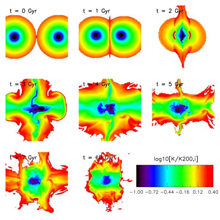
Figure 2: Logarithmic entropy slices (i.e., thickness of zero) through the centre of the default FLASH merger simulation (with $l=6$) at times 0, 1, 2, 3, 4, 5, 7 and 10 Gyr. The lowest entropy material is shown in blue, increasing in entropy through green, yellow to red. Each panel is 6 Mpc on a side. Significant entropy is generated at $t\approx 2$ Gyr when the cores collide and gas is squirted out, and again later on when this gas reaccretes.

A comparison of the left hand panel of Fig. 1 to Fig. 5 of VKB05 reveals a remarkable correspondence between the results of our idealised merger simulations and those of their cosmological simulations (which spanned system masses of $\sim 10^{13-15}M_{\odot}$). They find that the ratio of the AMR and SPH core amplitudes is $\sim 2$ in both the idealised and cosmological simulations. This difference is also seen in the Santa Barbara comparison of Frenk et al. (1999) when comparisons are made between the SPH simulations and the highest resolution AMR simulations carried out in that study (ie., the ‘Bryan’ AMR results). This consistency presumably indicates that whatever mechanism is responsible for the differing core amplitudes in the cosmological simulations is also responsible for the differing core amplitudes in our idealised simulations. This is encouraging, as it implies the generation of the entropy cores can be studied with idealised simulations. As outlined in §1, the advantage of idealised simulations over cosmological simulations is their relative simplicity. This gives us hope that we can use idealised simulations to track down the underlying cause of the discrepancy between particle-based and mesh-based hydrodynamic codes.

The right hand panel of Figure 1 shows the resulting entropy distributions plotted in a slightly different fashion. Here we plot the entropy as a function of ‘enclosed’ gas mass $K(<M_{\rm gas})$. This is constructed by simply ranking the particles/cells by entropy in ascending order and then summing the masses of the particles/cells [the inverse, $M_{\rm gas}(K)$, would therefore be the total mass of gas with entropy lower than $K$]. Convective stability ensures that, eventually when the system is fully relaxed, the lowest-entropy gas will be located at the very centre of the potential well, while the highest entropy gas will be located at the system periphery. $K(<M_{\rm gas})$ is therefore arguably a more fundamental quantity than $K(r)$ and we adopt this test throughout the rest of the paper. It is also noteworthy that in order to compute $K(<M_{\rm gas})$ one does not first need to select a reference point (e.g., the centre of mass or the position of the particle with the lowest potential energy) or to bin the particles/cells in any way, both of which could introduce ambiguities in the comparison between the SPH and AMR simulations (albeit likely minor ones).

In the right hand panel of Figure 1, we plot the resulting $K(<M_{\rm gas})$ distributions normalised to the final entropy distribution of the default GADGET-2 run. Here we see that the lowest-entropy gas in the FLASH runs have a higher entropy, by a factor of $\approx 1.9-2.0$, than the lowest-entropy gas in the default GADGET-2 run. Naively, looking at the right hand panel of Figure 1 one might conclude that the discrepancy is fairly minor, given that $\sim 95$% of the gas has been heated to a similar degree in the SPH and AMR simulations. But it is important to keep in mind that it is the properties of the lowest-entropy gas in particular that are most relevant to the issue of heating vs. cooling in groups and clusters (and indeed in haloes of all masses), since this is the gas that has the shortest cooling time.

The agreement between our results and those from cosmological simulations (e.g., Frenk et al. 1999; VKB05) is striking. The convergence of the entropy distributions in our idealised simulations negates the explanation that inadequate resolution of the high redshift universe in cosmological AMR simulations is the root cause of the discrepancy between the entropy cores in SPH and AMR simulations (although we note that some of the lower resolution AMR simulations in the study of Frenk et al. may not have been fully converged and therefore the discrepancy may have been somewhat exaggerated in that study for those simulations). We therefore conclude that the higher entropy generation in AMR codes relative to SPH codes within the cores of groups and clusters arises out of a more fundamental difference in the adopted algorithms. Below we examine in more detail how the entropy is generated during the merging process in the simulations and we then systematically explore several possible causes for the differences in the simulations.

3.2 An overview of heating in the simulations

We have demonstrated that the entropy generation that takes place in our idealised mergers is robust to our choice of resolution, yet a difference persists in the amount of central entropy that is generated in the SPH and mesh simulations. We now examine the entropy generation as a function of time in the simulations, which may provide clues to the origin of the difference between the codes.

Figure 2 shows $\log(K)$ in a slice through the centre of the default FLASH simulation at times 0, 1, 2, 3, 4, 5, 7 and 10 Gyr. This may be compared to Figure 3, which shows the entropy distribution of the simulations as a function of time (this figure is described in detail below). Briefly, as the cores approach each other, a relatively gentle shock front forms between the touching edges of the clusters, with gas being forced out perpendicular to the collision axis. Strong heating does not actually occur until approximately the time when the cores collide, roughly 1.8 Gyrs into the run. The shock generated through the core collision propagates outwards, heating material in the outer regions of the system. This heating causes the gas to expand and actually overshoot hydrostatic equilibrium. Eventually, the gas, which remains gravitationally bound to the system, begins to fall back onto the system, producing a series of weaker secondary shocks. Gas at the outskirts of the system, which is the least bound, takes the longest to re-accrete. This dependence of the time for gas to be re-accreted upon the distance from the centre results in a more gradual increase in entropy than seen in the initial core collision. In a qualitative sense, the heating process that takes place in the FLASH simulations is therefore very similar to that seen in the GADGET-2 simulations (see §3 of McCarthy et al. 2007 for an overview of the entropy evolution in idealised GADGET-2 mergers).

The top left panel in Figure 3 shows the ratio of $K(<M_{\rm gas})$ in the default FLASH run relative to $K(<M_{\rm gas})$ in the default GADGET-2 run. The various curves represent the ratio at different times during the simulations (see figure key — note that these correspond to the same outputs displayed in Figure 2). It can clearly be seen that the bulk of the difference in the final entropy distributions of the simulations is established around the time of core collision. The ratio of the central entropy in the FLASH simulation to the central entropy in the GADGET-2 simulation converges after $\approx 4$ Gyr. The top right panel shows the time evolution of the lowest-entropy gas only in both the GADGET-2 and FLASH runs. Here we see there are similar trends with time, in the sense that there are two main entropy generation episodes (core collision and re-accretion), but that the entropy generated in the first event is much larger in the FLASH run than in the GADGET-2 run. Far outside the core, however, the results are very similar. For completeness, the bottom two panels show $K(<M_{\rm gas})$ at different times for the GADGET-2 and FLASH runs separately.

The small initial drop in the central entropy at 1 Gyr in the FLASH run (see bottom left panel) is most likely due to interpolation errors at low resolution. This drop in entropy should not physically occur without cooling processes (which are not included in our simulations), but there is nothing to prevent a dip from occurring in the simulations due to numerical inaccuracies (the second law of thermodynamics is not explicitly hardwired into the mesh code). At low resolutions, small violations in entropy conservation can occur due to inaccurate interpolations made by the code. We have verified that the small drop in entropy does not occur in the higher resolution FLASH runs. We note that while this effect is present in default FLASH run, it is small and as demonstrated in Fig. 1 the default run is numerically converged.

It is interesting that the FLASH to GADGET-2 central entropy ratio converges relatively early on in the simulations. This is in spite of the fact that a significant fraction of the entropy that is generated in both simulations is actually generated at later times, during the re-accretion phase. Evidently, this phase occurs in a very similar fashion in both simulations. In §4, we will return to the point that the difference between the results of the AMR and SPH simulations arises around the time of core collision.

Figure 3: The time-dependence of entropy generation in the default GADGET-2 and FLASH runs. The top left panel shows the ratio of $K(<M_{\rm gas})$ in the default FLASH run to $K(<M_{\rm gas})$ in the default GADGET-2 run. The various curves represent the ratio at different times during the simulations (see legend). The top right panel shows the time evolution of the lowest-entropy gas only in the default runs. Shown are $K(<M_{\rm gas}/M_{\rm gas,tot}=0.03)$ (thick curves) and $K(<M_{\rm gas}/M_{\rm gas,tot}=0.05)$ (thin curves) for the FLASH (long-dashed red curves) and GADGET-2 (solid blue curves) runs (i.e., having sorted the gas particles/cells by entropy, we show the evolution of the entropy that encloses 3% and 5% of the total gas mass). The curves have been normalised to their initial values at the start of the simulations. The short-dashed black curve represents the ratio of FLASH to GADGET-2 entropies enclosing 3% of the total gas mass. The bottom two panels show the $K(<M_{\rm gas})$ distributions for the default FLASH and GADGET-2 runs separately, at different times during the simulation. Together, these plots illustrate that the difference in the final entropy distributions of the FLASH and GADGET-2 runs is primarily established around the time of core collision ($\sim 2-3$ Gyr). It is worth noting, however, that significant entropy generation continues after this time, but it occurs in nearly the same fashion in the AMR and SPH runs.

3.3 Alternative setups

It is important to verify that the conclusions we have drawn from our default setup are not unique to that specific initial configuration. Using a suite of merger simulations of varying mass ratio and orbital parameters, McCarthy et al. (2007) demonstrated that the entropy generation that takes place does so in a qualitatively similar manner to that described above in all their simulations. However, these authors examined only SPH simulations. We have therefore run several additional merger simulations in both GADGET-2 and FLASH to check the robustness of our conclusions. All of these mergers are carried out using the same resolution as adopted for the default GADGET-2 and FLASH runs.

In Figure 4, we plot the final FLASH to GADGET-2 $K(<M_{\rm gas})$ ratio for equal mass mergers with varying orbital parameters (see figure caption). In all cases, FLASH systematically produces larger entropy cores than GADGET-2 , and by a similar factor to that seen in the default merger setup. Interestingly, the off-axis case results in a somewhat larger central entropy discrepancy between GADGET-2 and FLASH , even though the bulk energetics of this merger are the same as for the default case. A fundamental difference between the off-axis case and the default run is that the former takes a longer time for the cores to collide and subsequently relax (but note by the end of the off-axis simulation there is very little ongoing entropy generation, as in the default case). This may suggest that the timescale over which entropy is generated plays some role in setting the magnitude of the discrepancy between the AMR and SPH simulations. For example, one possibility is that ‘pre-shocking’ due to the artificial viscosity i.e., entropy generation during the early phases of the collision when the interaction is subsonic or mildly transonic) in the SPH simulations becomes more relevant over longer timescales. Another possibility is that mixing, which is expected to be more prevalent in Eulerian mesh simulations than in SPH simulations, plays a larger role if the two clusters spend more time in orbit about each other before relaxing into a single merged system (of course, one also expects enhanced mixing in the off-axis case simply because of the geometry). We explore these and other possible causes of the difference in §4.

In addition to varying the orbital parameters, we have also experimented with colliding a cluster composed of dark matter only with another cluster composed of a realistic mixture of gas and dark matter (in this case, we simulated the head on merger of two equal mass $10^{15}M_{\odot}$ clusters with an initial relative velocity of $\simeq 1444$ km/s). Obviously, this is not an astrophysically reasonable setup. However, a number of studies have suggested that there is a link between the entropy core in clusters formed in non-radiative cosmological simulations and the amount of energy exchanged between the gas and the dark matter in these systems (e.g., Lin et al. 2006; McCarthy et al. 2007). It is therefore interesting to see whether this experiment exposes any significant differences with respect to the results of our default merger simulation.

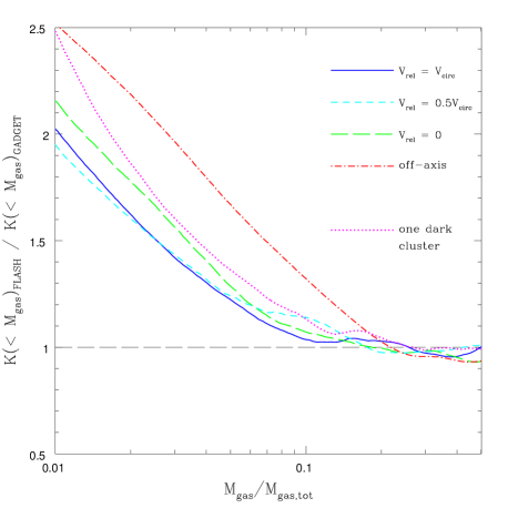
Figure 4: The ratio of FLASH to GADGET-2 final entropy distributions for equal mass mergers of varying initial orbital parameters. The solid blue curve represents the default setup (head on collision with an initial relative velocity of $V_{\rm circ}(r_{200})$). The long-dashed green and short-dashed cyan curves represent head on collisions with initial relative velocities of $0.5V_{\rm circ}(r_{200})$ and $0$ (i.e., at rest initially). The dot dashed red curve represents an off-axis collision with an initial relative radial velocity of $\simeq 0.95V_{\rm circ}(r_{200})$ and an initial relative tangential velocity of $\simeq 0.312V_{\rm circ}(r_{200})$ (i.e., the total energy is equivalent to that of the default setup). Also shown (dotted magenta curve), is the entropy ratio of a run where one of the clusters is composed of dark matter only and the other of a realistic mixture of gas and dark matter (see text). All these simulations result in a comparable difference in entropy profile between the mesh code and the SPH code.

The dotted magenta curve in Figure 4 represents the final FLASH to GADGET-2 $K(<M_{\rm gas})$ ratio for the case where a dark matter only cluster merges with another cluster composed of both gas and dark matter. The results of this test are remarkably similar to that of our default merger case. This indicates that the mechanism responsible for the difference in heating in the mesh and SPH simulations in the default merger simulation is also operating in this setup. Although this does not pin down the difference between the mesh and SPH simulations, it does suggest that the difference has little to do with differences in the properties of the large hydrodynamic shock that occurs at core collision, as there is no corresponding large hydrodynamic shock in the case where one cluster is composed entirely of dark matter. However, it is clear from Figure 3 that the difference between the default mesh and SPH simulations is established around the time of core collision, implying that some source of heating other than the large hydrodynamic shock is operating at this time (at least in the FLASH simulation). We return to this point in §4.

4 What Causes The Difference?

There are fundamental differences between Eulerian mesh-based and Lagrangian particle-based codes in terms of how they compute the hydrodynamic and gravitational forces. Ideally, in the limit of sufficiently high resolution, the two techniques would yield identical results for a given initial setup. Indeed, both techniques have been shown to match with high accuracy a variety of test problems with known analytic solutions. However, as has been demonstrated above (and in other recent studies; e.g., Agertz et al. 2007; Trac et al. 2007; Wadsley et al. 2008) differences that do not appear to depend on resolution present themselves in certain complex, but astrophysically-relevant, circumstances.

In what follows, we explore several different possible causes for why the central heating that takes place in mesh simulations exceeds that in the SPH simulations. The possible causes we explore include:

• § 4.1 A difference in gravity solvers - Most currently popular mesh codes (including FLASH and ENZO ) use a particle-mesh (PM) approach to calculate the gravitational force. To accurately capture short range forces it is therefore necessary to have a finely-sampled mesh. By contrast, particle-based codes (such as GADGET-2 and GASOLINE ) often make use of tree algorithms or combined tree particle-mesh (TreePM) algorithms, where the tree is used to compute the short range forces and a mesh is used to compute long range forces. Since the gravitational potential can vary rapidly during major mergers and large quantities of mass can temporarily be compressed into small volumes, it is conceivable differences in the gravity solvers and/or the adopted gravitational force resolution could give rise to different amounts of entropy generation in the simulations.

• § 4.2 Galilean non-invariance of mesh codes - Given explicit dependencies in the Riemann solver’s input states, all Eulerian mesh codes are inherently not Galilean invariant to some degree. This can lead to spurious entropy generation in the cores of systems as they merely translate across the simulation volume (e.g., Tasker et al. 2008).

• § 4.3 ‘Pre-shocking’ in the SPH runs - Artificial viscosity is required in SPH codes to capture the effects of shock heating. However, the artificial viscosity can in principle lead to entropy production in regions where no shocks should be present (e.g., Dolag et al. 2005). If such pre-shocking is significant prior to core collision in our SPH simulations, it could result in a reduced efficiency of the primary shock.

• § 4.4 A difference in the amount of mixing in SPH and mesh codes - Mixing will be suppressed in standard SPH implementations where steep density gradients are present, since Rayleigh-Taylor and Kelvin-Helmholtz instabilities are artificially damped in such circumstances (e.g., Agertz et al. 2007). In addition, the standard implementation of artificial viscosity will damp out even subsonic motions in SPH simulations, thereby inhibiting mixing (Dolag et al. 2005). On the other hand, one expects there to be some degree of over-mixing in mesh codes, since fluids are implicitly assumed to be fully mixed on scales smaller than the minimum cell size.
  
  We now investigate each of these possible causes in turn. We do not claim that these are the only possible causes for the differences we see in the simulations. They do, however, represent the most commonly invoked possible solutions (along with hydrodynamic resolution, which we explored in §3) to the entropy core discrepancy between SPH and mesh codes.

4.1 Is it due to a difference in the gravity solvers?

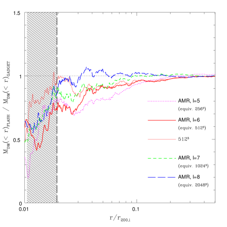
Figure 5: A plot comparing the resulting dark matter mass distributions for the default merger setup at 10 Gyr. The dark matter mass profiles have been normalised to the final dark matter mass profile of the default resolution GADGET-2 run. The dotted magenta, solid red, short-dashed green, and long-dashed blue curves represent the FLASH AMR runs with $l=$ 5, 6, 7, and 8, respectively, which correspond to peak grid cell sizes of $\approx 78$, $39$, $19.5$, and $9.8$ kpc (respectively). The thin solid red curve represents the uniform $512^{3}$ FLASH run. The gravitational softening length adopted for the GADGET-2 run is 10 kpc. For reference, $r_{200,i}\simeq 2062$ kpc. The vertical dashed line indicates four softening lengths. The FLASH dark matter distribution converges to the GADGET-2 result when the numerical resolutions become similar: the observed differences in gas entropy are not due to differences in the underlying dark matter dynamics.

In the FLASH simulations, gravity is computed using a standard particle-mesh approach. With this approach, the gravitational force will be computed accurately only on scales larger than the finest cell size. By contrast, the GADGET-2 simulations make use of a combined TreePM approach, where the tree algorithm computes the short range gravitational forces and the particle-mesh algorithm is used only to compute long range forces. To test whether or not differences in the gravity solvers (and/or gravitational force resolution) are important, we compare the final mass distributions of the dark matter in our simulations. The distribution of the dark matter should be insensitive to the properties of the diffuse baryonic component, since its contribution to the overall mass budget is small by comparison to the dark matter. Thus, the final distribution of the dark matter tells us primarily about the gravitational interaction alone between the two clusters.

Figure 5 shows the ratio of the final FLASH dark matter mass profiles to the final GADGET-2 dark matter mass profile. Recall that in all runs the number of dark matter particles is the same. The differences that are seen in this figure result from solving for gravitational potential on a finer mesh. For the lowest resolution FLASH run, we see that the final dark matter mass profile deviates significantly from that of the default GADGET-2 run for $r\la 0.04r_{200,i}$. However, this should not be surprising, as the minimum cell size in the default FLASH run is $\sim 0.02r_{200,i}$. By increasing the maximum refinement level, $l$, we see that the discrepancy between the final FLASH and GADGET-2 dark matter mass profiles is limited to smaller and smaller radii. With $l=8$, the minimum cell size is equivalent to the gravitational softening length adopted in the default GADGET-2 run. In this case, the final dark matter mass distribution agrees with that of the default GADGET-2 run to within a few percent at all radii beyond a few softening lengths (or a few cell sizes), which is all that should be reasonably expected. A comparison of the various FLASH runs with one another (compare, e.g., the default FLASH run with the $l=8$ run, for which there is a $\sim 6$% discrepancy out as far as $0.1r_{200}$) may suggest a somewhat slower rate of convergence to the default GADGET-2 result than one might naively have expected. Given that we have tested the new FFT gravity solver against both the default multigrid solver and a range of simple analytic problems and confirmed its accuracy to a much higher level than this, we speculate that the slow rate of convergence is due to the relatively small number of dark matter particles used in the mesh simulations. In the future, it would be useful to vary the number of dark matter particles in the mesh simulations to verify this hypothesis.

In summary, we find that the resulting dark matter distributions agree very well in the GADGET-2 and FLASH simulations when the effective resolutions are comparable. The intrinsic differences between the solvers therefore appear to be minor. More importantly for our purposes, even though the gravitational force resolution for the default FLASH run is not as high as for the default GADGET-2 run, this has no important consequences for the comparison of the final entropy distributions of the gas. It is important to note that, even though the final mass distribution in the FLASH simulations shows small differences between $l=6$ and 8, Figure 1 shows that the entropy distribution is converged for $l\geq 6$ and is not at all affected by the improvement in the gravitational potential.

4.2 Is it due to Galilean non-invariance of grid hydrodynamics?

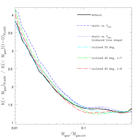
Figure 6: Testing the effects of Galilean non-invariance on the FLASH merger simulations. Plotted is the final entropy distribution, normalised to the initial one, for the default FLASH merger simulation and various different ‘takes’ on the default run. The solid black curve represents the default run, the short-dashed blue curves represents a merger where one cluster is held static and the other given a bulk velocity twice that in the default run (i.e., the relative velocity is unchanged from the default run), and the dotted blue curve represents this same merger but with the size of the time steps reduced by an order of magnitude. The dashed cyan, green, and red lines represent mergers that take place on an oblique angle to mesh at 33 degrees, 45 degrees with $l=7$ and 45 degrees with $l=8$, respectively. This comparison illustrates that the effects of Galilean non-invariance on the resulting entropy distribution are minor and do not account for the difference in the entropy core amplitudes of the mesh and SPH simulations.

Due to the nature of Riemann solvers (which are a fundamental feature of AMR codes), it is possible for the evolution of a system to be Galilean non-invariant. This arises from the fixed position of the grid relative to the fluid. The Riemann shock tube initial conditions are constructed by determining the amount of material that can influence the cell boundary from either side, within a given time step based on the sound speed. The Riemann problem is then solved at the boundary based on the fluid properties either side of the boundary. By applying a bulk velocity to the medium in a given direction, the nature of the solution changes. Although an ideal solver would be able to decouple the bulk velocity from the velocity discontinuity at the shock, the discrete nature of the problem means that the code may not be Galilean invariant. Since one expects large bulk motions to be relevant for cosmological structure formation, and clearly is quite relevant for our merger simulations, it is important to quantify what effects (if any) Galilean non-invariance has on our AMR simulations.

We have tested the Galilean non-invariance of our FLASH simulations in two ways. In the first test, we simulate an isolated cluster moving across the mesh with an (initial) bulk velocity of $V_{\rm circ}(r_{200})$ ($\simeq 1444$ km/s) and compare it to an isolated cluster with zero bulk velocity. This is similar to the test carried out recently by Tasker et al. (2008). In agreement with Tasker et al. (2008), we find that there is some spurious generation of entropy in the very central regions ($M_{\rm gas}/M_{\rm gas,tot}\la 0.03$) of the isolated cluster that was given an initial bulk motion. However, after $\approx 2$ Gyr of evolution (i.e., the time when the clusters collide in our default merger simulation), the increase in the central entropy is only $\sim 10$%. This is small in comparison to the $\sim 300$% jump that takes place at core collision in our merger simulations. This suggests that spurious entropy generation prior to the merger is minimal and does not account for the difference we see between the SPH and AMR simulations.

In the second test, we consider different implementations of the default merger simulation. In one case, instead of giving both systems equal but opposite bulk velocities (each with magnitude $0.5V_{\rm circ}$), we fix one and give the other an initial velocity that is twice the default value, so that the relative velocity is unchanged. (We also tried reducing the size of the time steps for this simulation by an order magnitude.) In addition, we have tried mergers that take place at oblique angles relative to the grid. If the merger is well-resolved and the dynamics are Galilean invariant, all these simulations should yield the same result.

Figure 6 shows the resulting entropy distributions for these different runs. The results of this test confirm what was found above; i.e., that there is some dependence on the reference frame adopted, but that this effect is minor in general (the central entropy is modified by $\la 10$%) and does not account for the discrepancy we see between entropy core amplitudes in the default GADGET-2 and FLASH simulations.

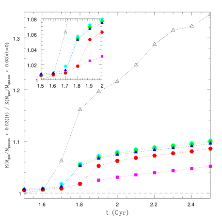
Figure 7: Testing the effects of pre-shocking due to artificial viscosity in the default GADGET-2 merger simulation. This plot shows the evolution of the central entropy (enclosing 3% of the gas mass) around the time of first core collision. The solid blue triangles represent the default GADGET-2 simulation. The solid cyan points, solid green points, and solid red points represent runs where the artificial viscosity is kept at a very low level ($\alpha_{\rm visc}=0.05$) until $t\approx$ 1.6, 1.7, 1.8 Gyr, respectively, at which point the artificial viscosity is set back to its default value. The solid magenta squares represent a run with low artificial viscosity throughout, and the open triangles represent the default FLASH simulation. Reducing the value of the artificial viscosity parameter before the cores collide delays the increase in entropy (cyan, green and solid red), however as soon as the original value is restored, the entropy $K$ increases to a level nearly independent of when $\alpha$ was restored. Therefore pre-shocking has little effect on the post-shock value of $K$.

4.3 Is it due to ‘pre-shocking’ in SPH?

Artificial viscosity is required in SPH codes in order to handle hydrodynamic shocks. The artificial viscosity acts as an excess pressure in the equation of motion, converting gas kinetic energy into internal energy, and therefore raising the entropy of the gas. In standard SPH implementations, the magnitude of the artificial viscosity is fixed in both space and time for particles that are approaching one another (it being set to zero otherwise). This implies that even in cases where the Mach number is less than unity, i.e., where formally a shock should not exist, (spurious) entropy generation can occur. This raises the possibility that significant ‘pre-shocking’ could occur in our SPH merger simulations. This may have the effect of reducing the efficiency of the large shock that occurs at core collision and could therefore potentially explain the discrepancy between the mesh and SPH simulations.

Figure 8: Quantifying the amount of heating and mixing in the default GADGET-2 and FLASH merger simulations. Left: The entropy of particles (tracer particles in the case of FLASH ) at time $t$ vs. the initial entropy of those particles. The solid green line is the line of equality [$K(t)=K(t=0)$; i.e., no heating]. The shaded blue and red regions represent the distributions from the GADGET-2 and FLASH simulations, respectively. They enclose 50% of the particles; i.e., the lower/upper bounds represent the 25th/75th percentiles for $K(t)$ at fixed $K(t=0)$. The dashed blue and red lines represent the median $K(t)$ at fixed $K(t=0)$. The central entropy in the FLASH runs increases significantly more than in the GADGET-2 run when the cores collide, at $t\sim 2$ Gyr, the increase in entropy later is similar between the two codes. The scatter in FLASH entropy is also much larger than in GADGET-2 . Right: The enclosed gas mass of particles (tracers particles in the case of FLASH ) at time $t$ vs. the initial enclosed mass of those particles. The enclosed gas mass of each particle is calculated by summing the masses of all other particles (or cells) with entropies lower than the particle under consideration. The solid green line is the line of equality [$M_{\rm gas}(t)=M_{\rm gas}(t=0)$; i.e., no mass mixing]. The shaded blue and red regions represent the distributions from the GADGET-2 and FLASH simulations, respectively. They enclose 50% of the particles; i.e., the lower/upper bounds represent the 25th/75th percentiles for $M_{\rm gas}(t)$ at fixed $M_{\rm gas}(t=0)$. The dashed blue and red lines represent the median $M_{\rm gas}(t)$ at fixed $M_{\rm gas}(t=0)$. Particles in FLASH mix much more than in GADGET-2 .

Dolag et al. (2005) raised this possibility and tested it in SPH cosmological simulations of massive galaxy clusters. They implemented a new variable artificial viscosity scheme by embedding an on-the-fly shock detection algorithm in GADGET-2 that indicates if particles are in a supersonic flow or not. If so, the artificial viscosity is set to a typical value, if not the artificial viscosity is greatly reduced. This new implementation should significantly reduce the amount of pre-shocking that takes place during formation of the clusters. The resulting clusters indeed had somewhat higher central entropies relative to clusters simulated with the standard artificial viscosity implementation (although the new scheme does not appear to fully alleviate the discrepancy between mesh and SPH codes). However, whether the central entropy was raised because of the reduction in pre-shocking or if it was due to an increase in the amount of mixing is unclear.

Our idealised mergers offer an interesting opportunity to re-examine this test. In particular, because of the symmetrical geometry of the merger, little or no mixing is expected until the cores collide, as prior to this time there is no interpenetration of the gas particles belonging to the two clusters (we have verified this). This means that we are in a position to isolate the effects of pre-shocking from mixing early on in the simulations. To do so, we have devised a crude method meant to mimic the variable artificial viscosity scheme of Dolag et al. (2005). In particular, we run the default merger with a low artificial viscosity (with $\alpha_{\rm visc}=0.05$, i.e., approximately the minimum value adopted by Dolag et al. ) until the cores collide, at which point we switch the viscosity back to its default value. We then examine the amount of entropy generated in the large shock.

Figure 7 shows the evolution of the central entropy around the time of core collision. Shown are a few different runs where we switch the artificial viscosity back to its default value at different times (since the exact time of ‘core collision’ is somewhat ill-defined). Here we see that prior to the large shock very little entropy has been generated, which is expected given the low artificial viscosity adopted up to this point. A comparison of these runs to the default GADGET-2 simulation (see inset in Figure 7) shows that there is evidence for a small amount of pre-shocking in the default run. However, we find that for the cases where the artificial viscosity is set to a low value, the resulting entropy jump (after the viscosity is switched back to the default value) is nearly the same as in the default merger simulation. In other words, pre-shocking appears to have had a minimal effect on the strength of the heating that occurs at core collision in the default SPH simulation. This argues against pre-shocking as the cause of the difference we see between the mesh and SPH codes.

Lastly, we have also tried varying $\alpha_{\rm visc}$ over the range $0.5$ and $1.0$ (i.e., values typically adopted in SPH studies; Springel 2005b) for the default GADGET-2 run. We find that the SPH results are robust to variations in $\alpha_{\rm visc}$ and cannot reconcile the differences between SPH and AMR results.

Figure 9: The final spatial distribution of particles (tracer particles in the case of FLASH ) with the lowest initial entropies (we select the central 5% of particles/tracer particles in both clusters). The blue points represent particles belonging to one of the clusters and the red points represent particles belonging to the other. Left: The low resolution GADGET-2 simulation. Right: The default FLASH simulation. There is a high degree of mixing in the mesh simulation, whereas there remain two distinct blobs corresponding to the infallen clusters in the SPH simulation. The difference arises immediately following core collision through the turbulent mixing that it drives.

4.4 Is it due to a difference in the amount of mixing in SPH and mesh codes?

Our experiments with off-axis collisions and collisions with a cluster containing only dark matter suggest that mixing plays an important role in generating the differences between the codes. Several recent studies (e.g., Dolag et al. 2005; Wadsley et al. 2008) have argued that mixing is handled poorly in standard implementations of SPH, both because (standard) artificial viscosity acts to damp turbulent motions and because the growth of KH and RT instabilities is inhibited in regions where steep density gradients are present (Agertz et al. 2007). Using cosmological SPH simulations that have been modified in order to enhance mixing, Dolag et al. (2005) and Wadsley et al. (2008) have shown that it is possible to generate higher central entropies in their galaxy clusters (relative to clusters simulated using standard implementations of SPH), yielding closer agreement with the results of cosmological mesh simulations. This is certainly suggestive that mixing may be the primary cause of the discrepancy between mesh and SPH codes. However, these authors did not run mesh simulations of galaxy clusters and therefore did not perform a direct comparison of the amount of mixing in SPH vs. mesh simulations of clusters. Even if one were to directly compare cosmological SPH and mesh cluster simulations, the complexity of the cosmological environment and the hierarchical growth of clusters would make it difficult to clearly demonstrate that mixing is indeed the difference.

Our idealised mergers offer a potentially much cleaner way to test the mixing hypothesis. To do so, we re-run the default FLASH merger simulation but this time we include a large number of ‘tracer particles’, which are massless and follow the hydrodynamic flow of the gas during the simulation. The tracer particles are advanced using a second order accurate predictor-corrector time advancement scheme with the particle velocities being interpolated from the grid (further details are given in the flash manual (version 2.5) at:
http://flash.uchicago.edu/). Each tracer particle has a unique ID that is preserved throughout the simulation, allowing us to track the gas in a Lagrangian fashion, precisely as is done in Lagrangian SPH simulations. To simplify the comparison further, we initially distribute the tracer particles within the two clusters in our FLASH simulation in exactly the same way as the particles in our initial GADGET-2 setup.

In the left hand panel of Figure 8, we plot the final vs. the initial entropy of particles in the default GADGET-2 and FLASH merger simulations. This plot clearly demonstrates that the lowest-entropy gas is preferentially heated in both simulations, however the degree of heating of that gas in the mesh simulation is much higher than in the SPH simulation. Consistent with our analysis in §3, we find that the bulk of this difference is established around the time of core collision. It is also interesting that the scatter in the final entropy (for a given initial entropy) is much larger in the mesh simulation. The larger scatter implies that convective mixing is more prevalent in the mesh simulation. At or immediately following core collision ($t\approx 2-3$ Gyr), there is an indication that, typically, gas initially at the very centre of the two clusters (which initially had the lowest entropy) has been heated more strongly than gas further out [compare, e.g., the median $K(t=5{\rm Gyr})$ at $K(t=0)/K_{200,i}\approx 0.02$ to the median at $K(t=0)/K_{200,i}\approx 0.08$]. Such an entropy inversion does not occur in the SPH simulations and likely signals that the extra mixing in the mesh simulation has boosted entropy production.

Figure 10: Logarithmic projected entropy maps of the default GADGET-2 simulation and FLASH simulation with $l=8$ at $t=2.3$ Gyr, just after the collision of the cores. Note that the peak spatial resolutions of the two simulations are similar (approx. 10 kpc; we also note that the median SPH smoothing length for the default GADGET-2 run is $\approx 20$ kpc within the mixing region, $r\la 200$ kpc.) To highlight the central regions, we have reset the value of any pixel with projected entropy greater than $0.5K_{200,i}$ to $0.5K_{200,i}$. In these maps, the minimum entropy (black) is $\approx 0.07K_{200,i}$ and the maximum entropy (white) is $0.5K_{200,i}$. The maps are 2 Mpc on a side, and project over a depth of 2 Mpc. Note that the images are not directly comparable with figure 2, where a slice is shown. Left: the GADGET-2 simulation. Right: the FLASH simulation. The FLASH entropy distribution is characterised by vortices on a range of scales, which mix gas with different entropies. These vortices are mostly absent in the GADGET-2 simulation.

In the right hand panel of Figure 8 we plot the final vs. the initial enclosed gas mass of particles in the default GADGET-2 and FLASH merger simulations. The enclosed gas mass of each particle (or tracer particle) is calculated by summing the masses of all other particles (or cells) with entropies lower than the particle under consideration. This plot confirms our mixing expectations based on the entropy plot in the left hand panel. In particular, only a small amount of mass mixing is seen in the SPH simulation, whereas in the mesh simulation the central $\sim 5\%$ of the gas mass has been fully mixed.

The higher degree of mixing in the FLASH simulation is shown pictorially in Figure 9. The left panel shows the final spatial distribution of the initially lowest-entropy particles in GADGET-2 simulation, while the right panel is the analogous plot for tracer particles in the FLASH simulation (see figure caption). The larger degree of mixing in the mesh simulation relative to the SPH simulation is clearly evident. In the FLASH simulation, particles from the two clusters are intermingled in the final state, while distinct red and blue regions are readily apparent in the SPH calculation, a difference which arises immediately following core collision.

The increased mixing boosts entropy production in the FLASH simulations, but what is the origin of the increased mixing? We now return to the point raised in §3, that the bulk of the difference between mesh and SPH simulation is established around the time of core collision. This is in spite of the fact that significant entropy generation proceeds in both simulations until $t\sim 6$ Gyr. Evidently, both codes treat the entropy generation in the re-accretion phase in a very similar manner. What is different about the initial core collision phase? As pointed out recently by Agertz et al. (2007), SPH suppresses the growth of instabilities in regions where steep density gradients are present due to spurious pressure forces acting on the particles. Could this effect be responsible for the difference we see? To test this idea, we generate 2D projected entropy maps of the SPH and mesh simulations to search for signs of clear instability development. In the case of the SPH simulation, we first smooth the particle entropies (and densities) onto a 3D grid using the SPH smoothing kernel and the smoothing lengths of each particle computed by GADGET-2 . We then compute a gas mass-weighted projected entropy by projecting along the $z$-axis. In the case of the FLASH simulation, the cell entropies and densities are interpolated onto a 3D grid and projected in the same manner as for the GADGET-2 simulation.

Figure 10 shows a snap shot of the two simulations at $t=2.3$ Gyr, just after core collision. Large vortices and eddies are easily visible in the projected entropy map of the FLASH simulation but none are evident in the GADGET-2 simulation. In order to study the duration of these eddies, we have generated 100 such snap shots for each simulation, separated by fixed 0.1 Gyr intervals. Analysing the projected entropy maps as a movie, we find that these large vortices and eddies persist in the FLASH simulation from $t\approx 1.8-3.2$ Gyr. This corresponds very well with the timescale over which the difference between the SPH and mesh codes is established (see, e.g., the dashed black curve in the top right panel of Figure 3).

We therefore conclude that extra mixing in the mesh simulations, brought on by the growth of instabilities around the time of core collision, is largely responsible for the difference in the final entropy core amplitudes between the mesh and SPH simulations. Physically, one expects the development of such instabilities, since the KH timescale, $\tau_{\rm KH}$, is relatively short at around the time of core collision. We therefore conclude that there is a degree of under-mixing in the SPH simulations Whether or not the FLASH simulations yield the correct result, however, is harder to ascertain. As fluids are forced to numerically mix on scales smaller than the minimum cell size, it is possible that there is a non-negligible degree of over-mixing in the mesh simulations. Our resolution tests (see §3) show evidence for the default mesh simulation being converged, but it may be that the resolution needs to be increased by much larger factors than we have tried (or are presently accessible with current hardware and software) in order to see a difference.

5 Summary and Discussion

In this paper, we set out to investigate the origin of the discrepancy in the entropy structure of clusters formed in Eulerian mesh-based simulations compared to those formed in Lagrangian SPH simulations. While SPH simulations form clusters with almost powerlaw entropy distributions down to small radii, Eulerian simulations form much larger cores with the entropy distribution being truncated at significantly higher values. Previously it has been suspected that this discrepancy arose from the limited resolution of the mesh based methods, making it impossible for such codes to accurately trace the formation of dense gas structures at high redshift.

By running simulations of the merging of idealised clusters, we have shown that this is not the origin of the discrepancy. We used the GADGET-2 code (Springel 2005b) to compute the SPH solution and the FLASH code (Fryxell et al. 2000) to compute the Eulerian mesh solution. In these idealised simulations, the initial gas density structure is resolved from the onset of the simulations, yet the final entropy distributions are significantly different. The magnitude of the difference generated in idealised mergers is comparable to that seen in the final clusters formed in full cosmological simulations. A resolution study shows that the discrepancy in the idealised simulations cannot be attributed to a difference in the effective resolutions of the simulations. Thus, the origin of the discrepancy must lie in the code’s different treatments of gravity and/or hydrodynamics.

We considered various causes in some detail. We found that the difference was not due to:

• The use of different gravity solvers. The two codes differ in that GADGET-2 uses a TreePM method to determine forces, while FLASH uses the PM method alone. The different force resolutions of the codes could plausibly lead to differences in the energy transfer between gas and dark matter. Yet we find that the dark matter distributions produced by the two codes are almost identical when the mesh code is run at comparable resolution to the SPH code.

• Galilean non-invariance of mesh codes. We investigate whether the results are changed if we change the rest-frame defined by the hydrodynamic mesh. Although we find that an artificial core can be generated in this way in the mesh code, its size is much smaller than the core formed once the clusters collide, and is not enough to explain the difference between FLASH and GADGET-2 . We show that most of this entropy difference is generated in the space of $\sim 1$ Gyr when the cluster cores first collide.

• Pre-shocking in SPH. We consider the possibility that the artificial viscosity of the SPH method might generate entropy in the flow prior to the core collision, thus reducing the efficiency with which entropy is generated later. By greatly reducing the artificial viscosity ahead of the core collision, we show that this effect is negligible.

Having shown that none of these numerical issues can explain the difference of the final entropy distributions, we investigated the role of fluid mixing in the two codes. Several recent studies (e.g., Dolag et al. 2005; Wadsley et al. 2008) have argued that if one increases the amount of mixing in SPH simulations the result is larger cluster entropy cores that resemble the AMR results. While this is certainly suggestive, it does not clearly demonstrate that it is the enhanced mixing in mesh simulations that is indeed the main driver of the difference (a larger entropy core in the mesh simulations need not necessarily have been established by mixing). By injecting tracer particles into our FLASH simulations, we have been able to make an explicit comparison of the amount of mixing in the SPH and mesh simulations of clusters. We find very substantial differences. In the SPH computation, there is a very close relation between the initial entropy of a particle and its final entropy. In contrast, tracer particles in the FLASH simulation only show a close connection for high initial entropies. The lowest $\sim 5$% of gas (by initial entropy) is completely mixed in the FLASH simulation. We conclude that mixing and fluid instabilities are the cause of the discrepancy between the simulation methods.

The origin of this mixing is closely connected to the suppression of turbulence in SPH codes compared to the Eulerian methods. This can easily be seen by comparing the flow structure when the clusters collide: while the FLASH image is dominated by large scale eddies, these are absent from the SPH realisation (see Figure 10). It is now established that SPH codes tend to suppress the growth of Kelvin-Helmholtz instabilities in shear flows, and this seems to be the origin of the differences in our simulation results (e.g., Agertz et al. 2007). These structures result in entropy generation through mixing, an irreversible process whose role is underestimated by the SPH method. Of course, it is not clear that the turbulent structures are correctly captured in the mesh simulations (Iapichino & Niemeyer 2008; Wadsley et al. 2008). The mesh forces fluids to be mixed on the scale of individual cells. In nature, this is achieved through turbulent cascades that mix material on progressively smaller and smaller scales: the mesh code may well overestimate the speed and effectiveness of this process. Ultimately, deep X-ray observations may be able to tell us whether the mixing that occurs in the mesh simulations is too efficient. An attempt at studying large-scale turbulence in clusters was made recently by Schuecker et al. (2004). Their analysis of XMM-Newton observations of the Coma cluster indicated the presence of a scale-invariant pressure fluctuation spectrum on scales of 40-90 kpc and found that it could be well described by a projected Kolmogorov/Oboukhov-type turbulence spectrum. If the observed pressure fluctuations are indeed driven by scale-invariant turbulence, this would suggest that current mesh simulations have the resolution required to accurately treat the turbulent mixing process. Alternatively, several authors have suggested that ICM may be highly viscous (eg., Fabian et al. 2003) with the result that fluid instabilities will be strongly suppressed by physical processes. This might favour the use of SPH methods which include a physical viscosity (Sijacki & Springel 2006).

It is a significant advance that we now understand the origin of this long standing discrepancy. Our work also has several important implications. Firstly, as outlined in §1, there has been much discussion in the recent literature on the competition between heating and cooling in galaxy groups and clusters. The current consensus is that heating from AGN is approximately sufficient to offset cooling losses in observed cool core clusters (e.g., McNamara & Nulsen 2007). However, observed present-day AGN power output seems energetically incapable of explaining the large number of systems that do not possess cool cores (McCarthy et al. 2008). Recent high resolution X-ray observations demonstrate that these systems have higher central entropies than typical cool core clusters (e.g., Dunn & Fabian 2008). One way of getting around the energetics issue is to invoke an early episode of preheating (e.g., Kaiser 1991; Evrard & Henry 1991). Energetically, it is more efficient to raise the entropy of the (proto-)ICM prior to it having fallen into the cluster potential well, as its density would have been much lower than it is today (McCarthy et al. 2008). Preheating remains an attractive explanation for these systems.

However, as we have seen from our idealised merger simulations, the amount of central entropy generated in our mesh simulations is significant and is even comparable to the levels observed in the central regions of non-cool core clusters. It is therefore tempting to invoke mergers and the mixing they induce as an explanation for these systems. However, before a definitive statement to this effect can be made, much larger regions of parameter space should be explored. In particular, a much larger range of impact parameters and mass ratios is required, in addition to switching on the effects of radiative cooling (which we have neglected in the present study). This would be the mesh code analog of the SPH study carried out by Poole et al. (2006; see also Poole et al. 2008). We leave this for future work. Alternatively, large cosmological mesh simulations, which self-consistently track the hierarchical growth of clusters, would be useful for testing the merger hypothesis. Indeed, Burns et al. (2008) have recently carried out a large mesh cosmological simulation (with the ENZO code) and argue that mergers at high redshift play an important role in the establishment of present-day entropy cores. However, these results appear to be at odds with the cosmological mesh simulations (run with the ART code) of Nagai et al. (2007) (see also Kravtsov et al. 2005). These authors find that most of their clusters have large cooling flows at the present-day, similar to what is seen in some SPH cosmological simulations (e.g., Kay et al. 2004; Borgani et al. 2006). On the other hand, the SPH simulations of Keres et al. (2008) appear to yield clusters with large entropy cores. This may be ascribed to the lack of effective feedback in their simulations, as radiative cooling selectively removes the lowest entropy gas (see, e.g., Bryan 2000; Voit et al. 2002), leaving only high entropy (long cooling time) gas remaining in the simulated clusters. However, all the simulations just mentioned suffer from the overcooling problem (Balogh et al. 2001), so it is not clear to what extent the large entropy cores in clusters in either mesh or SPH simulations are produced by shock heating, overcooling, or both. All of these simulations implement different prescriptions for radiative cooling (e.g., metal-dependent or not), star formation, and feedback, and this may lie at the heart of the different findings. A new generation of cosmological code comparisons will be essential in sorting out these apparently discrepant findings. The focus should not only be on understanding the differences in the hot gas properties, but also on the distribution and amount of stellar matter, as the evolution of the cold and hot baryons are obviously intimately linked. Reasonably tight limits on the amount of baryonic mass in the form of stars now exists (see, e.g., Balogh et al.z 2008) and provides a useful target for the next generation of simulations. At present, merger-induced mixing as an explanation for intrinsic scatter in the hot gas properties of groups and clusters remains an open question.

Secondly, we have learnt a great deal about the nature of gas accretion and the development of hot gas haloes from SPH simulations of the universe. Since we now see that these simulations may underestimate the degree of mixing that occurs, which of these results are robust, which need revision? For example, Keres et al. (2005) (among others) have argued that cold accretion by galaxies plays a dominant role in fuelling the star formation in galaxies. Is it plausible that turbulent eddies could disrupt and mix such cold streams as they try to penetrate through the hot halo? We can estimate the significance of the effect by comparing the Kelvin-Helmholtz timescale, $\tau_{\rm KH}$, with the free-fall time, $\tau_{\rm FF}$. The KH timescale is given by (see, e.g., Nulsen 1982; Price 2008)

$$\tau_{\rm KH}\equiv\frac{2\pi}{\omega}$$ (7)

where

$$\omega=\frac{2\pi}{k}\frac{(\rho\rho^{\prime})^{1/2}v_{\rm rel}}{(\rho+\rho^{\prime})}$$ (8)

and $\rho$ is the density of the hot halo, $\rho^{\prime}$ is the density of the cold stream, $k$ is the wave number of the instability, and $v_{\rm rel}$ the velocity of the stream relative to the hot halo. If the stream and hot halo are in approximate pressure equilibrium, this implies a large density contrast (e.g., a $10^{4}$ K stream falling into a $10^{6}$ K hot halo of a Milky Way-type system would imply a density contrast of $100$). In the limit of $\rho^{\prime}\gg\rho$ and recognising that the mode responsible for the destruction of the stream is comparable to the size of the stream (i.e., $k\sim 2\pi/r^{\prime}$), eqns. (7) and (8) reduce to:

$$\tau_{\rm KH}\approx\frac{r^{\prime}}{v_{\rm rel}}\biggl{(}\frac{\rho^{\prime}}{\rho}\biggr{)}^{1/2}$$ (9)

Adopting $\rho^{\prime}/\rho=100$, $r^{\prime}=100$ kpc, and $v_{\rm rel}=200$ km/s (perhaps typical numbers for a cold stream falling into a Milky Way-type system), we find $\tau_{\rm KH}\sim 5$ Gyr. The free-fall time, $\tau_{\rm FF}=R_{\rm vir}/V_{\rm circ}(R_{\rm vir})$ [where $R_{\rm vir}$ is the virial radius of main system and $V_{\rm circ}(R_{\rm vir})$ is the circular velocity of the main system at its virial radius], is $\sim 1$ Gyr for a Milky Way-type system with mass $M_{\rm vir}\sim 10^{12}M_{\odot}$. On this basis, it seems that the stream would be stable because of the large density contrast in the flows. It is clear, however, that the universality of these effects need to be treated with caution, as the free-fall and KH timescales are not vastly discrepant. High resolution mesh simulations (cosmological or idealised) of Milky Way-like systems would provide a valuable check of the SPH results.

Finally, the SPH method has great advantages in terms of computational speed, effective resolution and Galilean invariance. Is it therefore possible to keep these advantages and add additional small scale transport processes to the code in order to offset the suppression of mixing? Wadsley et al. (2008) and Price (2008) have presented possible approaches based on including a thermal diffusion term in the SPH equations. Although the approaches differ in their mathematical details, the overall effect is the same. However, it is not yet clear how well this approach will work in cosmological simulations that include cooling (and feedback), since the thermal diffusion must be carefully controlled to avoid unphysical suppression of cooling in hydrostatic regions (e.g., Dolag et al. 2005). One possibility might be to incorporate such terms as a negative surface tension in regions of large entropy contrast (Hu & Adams 2006). An alternative approach is to combine the best features of the SPH method, such as the way that it continuously adapts to the local gas density and its flow, with the advantage of a Riemann based method of solving the fluid dynamic equations (e.g., Inutsuka 2002).

Clearly, there is a great need to find simple problems in which to test these codes: simple shock tube experiments are not sufficient because they do not include the disordered fluid motions that are responsible for generating the entropy core. Idealised mergers represent a step forward, but the problem is still not sufficiently simple that it is possible to use self-similar scaling techniques (e.g., Bertschinger 1985, 1989) to establish the correct solution . One possibility is to consider the generation of turbulent eddies in a fluctuating gravitational potential. We have begun such experiments, but (although the fluid flow patterns are clearly different) simply passing a gravitational potential through a uniform plasma at constant velocity does not expose the differences between SPH and Eulerian mesh based methods that we see in the idealised merger case. We will tackle the minimum complexity that is needed to generate these differences in a future paper.

References

- Agertz et al. (2007) Agertz O., et al., 2007, MNRAS, 380, 963
- Ascasibar & Markevitch (2006) Ascasibar, Y., & Markevitch, M. 2006, ApJ, 650, 102
- Ascasibar et al. (2003) Ascasibar, Y., Yepes, G., Müller, V., & Gottlöber, S. 2003, MNRAS, 346, 731
- Balogh et al. (2001) Balogh, M. L., Pearce, F. R., Bower, R. G., & Kay, S. T. 2001, MNRAS, 326, 1228
- Balogh et al. (2008) Balogh, M. L., McCarthy, I. G., Bower, R. G., & Eke, V. R. 2008, MNRAS, 385, 1003
- Benson et al. (2003) Benson, A. J., Bower, R. G., Frenk, C. S., Lacey, C. G., Baugh, C. M., & Cole, S. 2003, ApJ, 599, 38
- Benson (2005) Benson, A. J. 2005, MNRAS, 358, 551
- Bertschinger (1985) Bertschinger, E. 1985, ApJS, 58, 39
- Bertschinger (1989) Bertschinger E., 1989, ApJ, 340, 666
- Binney & Tabor (1995) Binney, J., & Tabor, G. 1995, MNRAS, 276, 663
- Borgani et al. (2005) Borgani, S., Finoguenov, A., Kay, S. T., Ponman, T. J., Springel, V., Tozzi, P., & Voit, G. M. 2005, MNRAS, 361, 233
- Borgani et al. (2006) Borgani, S., et al. 2006, MNRAS, 367, 1641
- Bower et al. (2006) Bower, R. G., Benson, A. J., Malbon, R., Helly, J. C., Frenk, C. S., Baugh, C. M., Cole, S., & Lacey, C. G. 2006, MNRAS, 370, 645
- Bower et al. (2008) Bower, R. G., McCarthy, I. G., & Benson, A. J. 2008, MNRAS, 390, 1399
- Bryan (2000) Bryan, G. L. 2000, ApJL, 544, L1
- Burns et al. (2008) Burns, J. O., Hallman, E. J., Gantner, B., Motl, P. M., & Norman, M. L. 2008, ApJ, 675, 1125
- Chen et al. (2007) Chen, Y., Reiprich, T. H., Böhringer, H., Ikebe, Y., & Zhang, Y.-Y., 2007, A&A, 466, 805C
- Colella & Woodward (1984) Colella, P., & Woodward, P. R. 1984, JCoPh, 54, 174
- Dolag et al. (2005) Dolag, K., Vazza, F., Brunetti, G., & Tormen, G., 2005, MNRAS, 364, 753D
- Dunn & Fabian (2008) Dunn, R. J. H., & Fabian, A. C. 2008, MNRAS, 385, 757
- Edge (2001) Edge, A. C. 2001, MNRAS, 328, 762
- Evrard & Henry (1991) Evrard, A. E., & Henry, J. P. 1991, ApJ, 383, 95
- Fabian (1994) Fabian, A. C. 1994, ARAA, 32, 277
- Fabian et al. (2003) Fabian A. C., Sanders J. S., Allen S. W., Crawford C. S., Iwasawa K., Johnstone R. M., Schmidt R. W., Taylor G. B., 2003, MNRAS, 344, L43
- Frenk et al. (1999) Frenk, C. S., et al. 1999, ApJ, 525, 554
- Fryxell et al. (2000) Fryxell, B., et al. 2000, ApJS, 131, 273
- Gingold & Monaghan (1977) Gingold, R. A., & Monaghan, J. J. 1977, MNRAS, 181, 375
- Gómez et al. (2002) Gómez, P. L., Loken, C., Roettiger, K., & Burns, J. O. 2002, ApJ, 569, 122
- Hu & Adams (2006) Hu, X. Y., & Adams, N. A., 2006 JCoPh, 213, 844H
- Iapichino & Niemeyer (2008) Iapichino L., Niemeyer J. C., 2008, MNRAS, 388, 1089
- Inutsuka (2002) Inutsuka S.-I., 2002, JCoPh, 179, 238
- Kaiser (1991) Kaiser, N. 1991, ApJ, 383, 104
- Kay et al. (2004) Kay, S. T., Thomas, P. A., Jenkins, A., & Pearce, F. R. 2004, MNRAS, 355, 1091
- Keres et al. (2005) Keres, D., Katz, N., Weinberg, D. H., & Davé, R. 2005, MNRAS, 363, 2
- Keres et al. (2008) Keres, D., Katz, N., Fardal, M., Dave, R., & Weinberg, D. H. 2008, MNRAS, submitted (arXiv:0809.1430)
- Kim et al. (2005) Kim, W.-T., El-Zant, A. A., & Kamionkowski, M. 2005, ApJ, 632, 157
- Kravtsov et al. (2005) Kravtsov, A. V., Nagai, D., & Vikhlinin, A. A. 2005, ApJ, 625, 588
- Lin et al. (2006) Lin, W. P., Jing, Y. P., Mao, S., Gao, L., & McCarthy, I. G. 2006, ApJ, 651, 636
- Löhner (1987) Löhner, R. 1987, Comp. Meth. App. Mech. Eng., 61, 323
- Lucy (1977) Lucy, L. B. 1977, AJ, 82, 1013
- McCarthy et al. (2004) McCarthy, I. G., Balogh, M. L., Babul, A., Poole, G. B., & Horner, D. J. 2004, ApJ, 613, 811
- McCarthy et al. (2007) McCarthy, I. G., et al. 2007, MNRAS, 376, 497
- McCarthy et al. (2008a) McCarthy, I. G., Babul, A., Bower, R. G., & Balogh, M. L. 2008, MNRAS, 386, 1309
- McCarthy et al. (2008b) McCarthy, I. G., Frenk, C. S., Font, A. S., Lacey, C. G., Bower, R. G., Mitchell, N. L., Balogh, M. L., & Theuns, T. 2008, MNRAS, 383, 593
- McNamara & Nulsen (2007) McNamara, B. R. & Nulsen, P. E. J. 2007, ARAA, 45, 117
- Monaghan (1992) Monaghan, J. J. 1992, ARAA, 30, 543
- Monaghan (1997) Monaghan, J. J. 1997, JCoPh, 136, 298
- Mori & Burkert (2000) Mori, M., & Burkert, A. 2000, ApJ, 538, 559
- Nagai et al. (2007) Nagai, D., Kravtsov, A. V., & Vikhlinin, A. 2007, ApJ, 668, 1
- Narayan & Medvedev (2001) Narayan, R., & Medvedev, M. V. 2001, ApJL, 562, L129
- Navarro et al. (1996) Navarro, J.F.,Frenk, C.S., & White, S.D.M. 1997, ApJ, 490, 493
- Navarro et al. (1997) Navarro, J.F., Frenk, C.S., & White, S.D.M. 1997, ApJ, 462, 563
- Neto et al. (2007) Neto, A. F., et al. 2007, MNRAS, 381, 1450
- Nulsen (1982) Nulsen, P. E. J. 1982, MNRAS, 198, 1007
- O’Shea et al. (2005) O’Shea, B. W., Nagamine, K., Springel, V., Hernquist, L., & Norman, M. L. 2005, ApJS, 160, 1
- Peterson et al. (2003) Peterson, J. R., Kahn, S. M., Paerels, F. B. S., Kaastra, J. S., Tamura, T., Bleeker, J. A. M., Ferrigno, C., & Jernigan, J. G. 2003, ApJ, 590, 207
- Poole et al. (2006) Poole, G. B., Fardal, M. A., Babul, A., McCarthy, I. G., Quinn, T., & Wadsley, J. 2006, MNRAS, 373, 881
- Poole et al. (2007) Poole, G. B., Babul, A., McCarthy, I. G., Fardal, M. A., Bildfell, C. J., Quinn, T., & Mahdavi, A. 2007, MNRAS, 380, 437
- Poole et al. (2008) Poole, G. B., Babul, A., McCarthy, I. G., Sanderson, A. J. R., & Fardal, M. A. 2008, MNRAS, in press (arXiv:0804.1552)
- Price (2008) Price, D. J. 2008, JCoPh, 227, 10040
- Ricker & Sarazin (2001) Ricker, P. M., & Sarazin, C. L. 2001, ApJ, 561, 621
- Ritchie & Thomas (2002) Ritchie, B. W., & Thomas, P. A. 2002, MNRAS, 329, 675
- Ruszkowski et al. (2004) Ruszkowski, M., Brüggen, M., & Begelman, M. C. 2004, ApJ, 611, 158
- Schuecker et al. (2004) Schuecker, P., Finoguenov, A., Miniati, F., Böhringer, H., & Briel, U. G. 2004, A&A, 426, 387
- Sijacki et al. (2008) Sijacki, D., Pfrommer, C., Springel, V., & Enßlin, T. A. 2008, MNRAS, 387, 1403
- Sijacki & Springel (2006) Sijacki D., Springel V., 2006, MNRAS, 371, 1025
- Springel et al. (2001) Springel, V., Yoshida, N., & White, S. D. M. 2001, New Astronomy, 6, 79
- Springel & Hernquist (2002) Springel, V., & Hernquist, L. 2002, MNRAS, 333, 649
- Springel (2005b) Springel, V. 2005, MNRAS, 364, 1105
- Springel et al. (2005a) Springel, V., White, S. D. M., Jenkins, A., et al., 2005a, Nature, 435, 629
- Steinmetz & White (1997) Steinmetz, M., & White, S. D. M. 1997, MNRAS, 288, 545
- Tasker et al. (2008) Tasker, E. J., Brunino, R., Mitchell, N. L., Michielsen, D., Hopton, S., Pearce, F. R., Bryan, G. L., & Theuns, T. 2008, MNRAS, 390, 1267
- Trac, Sills, & Pen (2007) Trac H., Sills A., Pen U.-L., 2007, MNRAS, 377, 997
- Voit et al. (2003) Voit, G. M., Balogh, M. L., Bower, R. G., Lacey, C. G., & Bryan, G. L. 2003, ApJ, 593, 272
- Voit & Donahue (1995) Voit, G. M., & Donahue, M. 1995, ApJ, 452, 164
- Voit & Donahue (2005) Voit, G. M., & Donahue, M. 2005, ApJ, 634, 955
- Voit et al. (2005) Voit, G. M., Kay, S. T., & Bryan, G. L. 2005, MNRAS, 364, 909
- Voit & Ponman (2003) Voit, G. M., & Ponman, T. J. 2003, ApJL, 594, L75
- Voit et al. (2002) Voit, G. M., Bryan, G. L., Balogh, M. L., & Bower, R. G. 2002, ApJ, 576, 601
- Wadsley, Veeravalli, & Couchman (2008) Wadsley J. W., Veeravalli G., Couchman H. M. P., 2008, MNRAS, 387, 427
- Younger & Bryan (2007) Younger, J. D., & Bryan, G. L. 2007, ApJ, 666, 647