Semidefinite geometry of the numerical range

Abstract

The numerical range of a matrix is studied geometrically via the cone of positive semidefinite matrices (or semidefinite cone for short). In particular it is shown that the feasible set of a two-dimensional linear matrix inequality (LMI), an affine section of the semidefinite cone, is always dual to the numerical range of a matrix, which is therefore an affine projection of the semidefinite cone. Both primal and dual sets can also be viewed as convex hulls of explicit algebraic plane curve components. Several numerical examples illustrate this interplay between algebra, geometry and semidefinite programming duality. Finally, these techniques are used to revisit a theorem in statistics on the independence of quadratic forms in a normally distributed vector.

Keywords: numerical range, semidefinite programming, LMI, algebraic plane curves

1 Notations and definitions

The numerical range of a matrix $A\in{\mathbb{C}}^{n\times n}$ is defined as

$${\mathcal{W}}(A)=\{w^{*}Aw\in{\mathbb{C}}\>:\>w\in{\mathbb{C}}^{n},\>w^{*}w=1\}.$$ (1)

It is a convex closed set of the complex plane which contains the spectrum of $A$. It is also called the field of values, see [7, Chapter 1] and [12, Chapter 1] for elementary introductions. Matlab functions for visualizing numerical ranges are freely available from [2] and [11].

Let

$$A_{0}=I_{n},\quad A_{1}=\frac{A+A^{*}}{2},\quad A_{2}=\frac{A-A^{*}}{2i}$$ (2)

with $I_{n}$ denoting the identity matrix of size $n$ and $i$ denoting the imaginary unit. Define

$${\mathcal{F}}(A)=\{y\in{\mathbb{P}}^{2}\>:\>F(y)=y_{0}A_{0}+y_{1}A_{1}+y_{2}A_{2}\succeq 0\}$$ (3)

with $\succeq 0$ meaning positive semidefinite (since the $A_{i}$ are Hermitian matrices, $F(y)$ has real eigenvalues for all $y$) and ${\mathbb{P}}^{2}$ denoting the projective real plane, see for example [8, Lecture 1]. Set ${\mathcal{F}}(A)$ is a convex cone, a linear section of the cone of positive semidefinite matrices (or semidefinite cone for short), see [1, Chapter 4]. Inequality $F(y)\succeq 0$ is called a linear matrix inequality (LMI). In the complex plane $\mathbb{C}$, or equivalently, in the affine real plane ${\mathbb{R}}^{2}$, set ${\mathcal{F}}(A)$ is a convex set including the origin, an affine section of the semidefinite cone.

Let

$$p(y)=\det(y_{0}A_{0}+y_{1}A_{1}+y_{2}A_{2})$$

be a trivariate form of degree $n$ defining the algebraic plane curve

$${\mathcal{P}}=\{y\in{\mathbb{P}}^{2}\>:\>p(y)=0\}.$$ (4)

Let

$${\mathcal{Q}}=\{x\in{\mathbb{P}}^{2}\>:\>q(x)=0\}$$ (5)

be the algebraic plane curve dual to $\mathcal{P}$, in the sense that we associate to each point $y\in\mathcal{P}$ a point $x\in\mathcal{Q}$ of projective coordinates $x=(\partial p(y)/\partial y_{0},\>\partial p(y)/\partial y_{1},\>\partial p(y)/\partial y_{2})$. Geometrically, a point in $\mathcal{Q}$ corresponds to a tangent at the corresponding point in $\mathcal{Q}$, and conversely, see [17, Section V.8] and [6, Section 1.1] for elementary properties of dual curves.

Let $\mathbb{V}$ denote a vector space equipped with inner product $\langle.,.\rangle$. If $x$ and $y$ are vectors then $\langle x,y\rangle=x^{*}y$. If $X$ and $Y$ are symmetric matrices, then $\langle X,Y\rangle=\mathrm{trace}(X^{*}Y)$. Given a set $\mathcal{K}$ in $\mathbb{V}$, its dual set consists of all linear maps from $\mathcal{K}$ to non-negative elements in $\mathbb{R}$, namely

$${\mathcal{K}}^{*}=\{y\in{\mathbb{V}}\>:\>\langle x,y\rangle\geq 0,\>x\in{\mathcal{K}}\}.$$

Finally, the convex hull of a set $\mathcal{K}$, denoted $\mathrm{conv}\>{\mathcal{K}}$, is the set of all convex combinations of elements in $\mathcal{K}$.

2 Semidefinite duality

After identifying $\mathbb{C}$ with ${\mathbb{R}}^{2}$ or ${\mathbb{P}}^{2}$, the first observation is that numerical range ${\mathcal{W}}(A)$ is dual to LMI set ${\mathcal{F}}(A)$, and hence it is an affine projection of the semidefinite cone.

Lemma 1

${\mathcal{W}}(A)={\mathcal{F}}(A)^{*}=\{\left(\langle A_{0},W\rangle,\>\langle A_{1},W\rangle,\>\langle A_{2},W\rangle\right)\in{\mathbb{P}}^{2}\>:\>W\in{\mathbb{C}}^{n\times n},\>W\succeq 0\}$.

Proof: The dual to ${\mathcal{F}}(A)$ is

$$\begin{array}[]{rcl}{\mathcal{F}}(A)^{*}&=&\{x\>:\>\langle x,y\rangle=\langle F(y),W\rangle=\sum_{k}\langle A_{k},W\rangle y_{k}\geq 0,\>W\succeq 0\}\\ &=&\{x\>:\>x_{k}=\langle A_{k},W\rangle,\>W\succeq 0\},\end{array}$$

an affine projection of the semidefinite cone. On the other hand, since $w^{*}Aw=w^{*}A_{1}w+i\>w^{*}A_{2}w$, the numerical range can be expressed as

$$\begin{array}[]{rcl}{\mathcal{W}}(A)&=&\{x=(w^{*}A_{0}w,\>w^{*}A_{1}w,\>w^{*}A_{2}w)\}\\ &=&\{x\>:\>x_{k}=\langle A_{k},W\rangle,\>W\succeq 0,\>\mathrm{rank}\>W=1\},\end{array}$$

the same affine projection as above, acting now on a subset of the semidefinite cone, namely the non-convex variety of rank-one positive semidefinite matrices $W=ww^{*}$. Since $w^{*}A_{0}w=1$, set ${\mathcal{W}}(A)$ is compact, and $\mathrm{conv}\>{\mathcal{W}}(A)={\mathcal{F}}(A)^{*}$. The equality ${\mathcal{W}}(A)={\mathcal{F}}(A)^{*}$ follows from the Toeplitz-Hausdorff theorem establishing convexity of ${\mathcal{W}}(A)$, see [12, Section 1.3] or [7, Theorem 1.1-2]. $\Box$

Lemma 1 indicates that the numerical range has the geometry of planar projections of the semidefinite cone. In the terminology of [1, Chapter 4], the numerical range is semidefinite representable.

3 Convex hulls of algebraic curves

In this section, we notice that the boundaries of numerical range ${\mathcal{W}}(A)$ and its dual LMI set ${\mathcal{F}}(A)$ are subsets of algebraic curves $\mathcal{P}$ and $\mathcal{Q}$ defined respectively in (4) and (5), and explicitly given as locii of determinants of Hermitian pencils.

3.1 Dual curve

Lemma 2

${\mathcal{F}}(A)$ is the connected component delimited by $\mathcal{P}$ around the origin.

Proof: A ray starting from the origin leaves LMI set ${\mathcal{F}}(A)$ when the determinant $p(y)=\det\>\sum_{k}y_{k}A_{k}$ vanishes. Therefore the boundary of ${\mathcal{F}}(A)$ is the subset of algebraic curve $\mathcal{P}$ belonging to the convex connected component containing the origin.$\Box$

Note that $\mathcal{P}$, by definition, is the locus, or vanishing set of a determinant of a Hermitian pencil. Moreover, the pencil is definite at the origin so the corresponding polynomial $p(y)$ satisfies a real zero (hyperbolicity) condition. Connected components delimited by such determinantal locii are studied in [9], where it is shown that they correspond to feasible sets of two-dimensional LMIs. A remarkable result of [9] is that every planar LMI set can be expressed this way. These LMI sets form a strict subset of planar convex basic semi-algebraic sets, called rigidly convex sets (see [9] for examples of convex basic semi-algebraic sets which are not rigidly convex). Rigidly convex sets are affine sections of the semidefinite cone.

3.2 Primal curve

Lemma 3

${\mathcal{W}}(A)=\mathrm{conv}\>{\mathcal{Q}}$.

Proof: From the proof of Lemma 1, a supporting line $\{x\>:\>\sum_{k}x_{k}y_{k}=0\}$ to ${\mathcal{W}}(A)$ has coefficients $y$ satisfying $p(y)=0$. The boundary of ${\mathcal{W}}(A)$ is therefore generated as an envelope of the supporting lines. See [15], [13, Theorem 10] and also [5, Theorem 1.3].$\Box$

${\mathcal{Q}}$ is called the boundary generating curve of matrix $A$ in [13]. An interesting feature is that, similarly to $\mathcal{P}$, curve $\mathcal{Q}$ can be expressed as the locus of a determinant of a Hermitian pencil. Following [5], given two matrices $A,B$ of size $m$-by-$n$ with respective entries $A_{r\>c}$ and $B_{r\>c}$, $r=1,\ldots,m$, $c=1,\ldots,n$, we define the second mixed compound $[A,B]$ of size $m(m-1)/2$-by-$n(n-1)/2$ as the matrix with entries

$$[A,B]_{R,C}=\frac{1}{2}(A_{r_{1}c_{1}}B_{r_{2}c_{2}}+A_{r_{2}c_{2}}B_{r_{1}c_{1}}-A_{r_{1}c_{2}}B_{r_{2}c_{1}}-A_{r_{2}c_{1}}B_{r_{1}c_{2}}).$$

with row indices $R=(r_{1},r_{2})$ and column indices $C=(c_{1},c_{2})$ corresponding to lexicographically ordered pairs such that $1\leq r_{1}<r_{2}\leq m$ and $1\leq c_{1}<c_{2}\leq n$.

Lemma 4

$$q(x)=\det\>\left[\begin{array}[]{cccc}0&x_{0}I_{n}&x_{1}I_{n}&x_{2}I_{n}\\ x_{0}I_{n}&[A_{0},A_{0}]&[A_{1},A_{0}]&[A_{0},A_{2}]\\ x_{1}I_{n}&[A_{1},A_{0}]&[A_{1},A_{1}]&[A_{1},A_{2}]\\ x_{2}I_{n}&[A_{2},A_{0}]&[A_{2},A_{1}]&[A_{2},A_{2}]\end{array}\right].$$

Proof: See [5, Theorem 2.4].$\Box$

Note that even though curve $\mathcal{Q}$ can be expressed as the determinantal locus of a Hermitian pencil, the pencil is not homogeneous and it cannot be definite. Hence the convex hull ${\mathcal{W}}(A)$ is not a rigidly convex LMI set, it cannot be an affine section of the semidefinite cone. However, as noticed in Lemma 1, it is an affine projection of the semidefinite cone.

4 Examples

4.1 Rational cubic and quartic

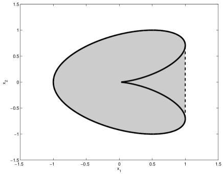
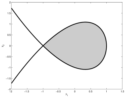
Figure 1: Left: LMI set ${\mathcal{F}}(A)$ (gray area) delimited by cubic $\mathcal{P}$ (black). Right: numerical range ${\mathcal{W}}(A)$ (gray area, dashed line) convex hull of quartic $\mathcal{Q}$ (black solid line).

Let

$$A=\left[\begin{array}[]{ccc}0&0&1\\ 0&1&i\\ 1&i&0\end{array}\right].$$

Then

$$F(y)=\left[\begin{array}[]{ccc}y_{0}&0&y_{1}\\ 0&y_{0}+y_{1}&y_{2}\\ y_{1}&y_{2}&y_{0}\end{array}\right]$$

and

$$p(y)=(y_{0}-y_{1})(y_{0}+y_{1})^{2}-y_{0}y^{2}_{2}$$

defines a genus-zero cubic curve $\mathcal{P}$ whose connected component containing the origin is the LMI set ${\mathcal{F}}(A)$, see Figure 1. With an elimination technique (resultants or Gröbner basis with lexicographical ordering), we obtain

$$q(x)=4x^{4}_{1}+32x^{4}_{2}+13x^{2}_{1}x^{2}_{2}-18x_{0}x_{1}x^{2}_{2}+4x_{0}x^{3}_{1}-27x^{2}_{0}x^{2}_{2}$$

defining the dual curve $\mathcal{Q}$, a genus-zero quartic with a cusp, whose convex hull is the numerical range ${\mathcal{W}}(A)$, see Figure 1.

4.2 Couple of two nested ovals

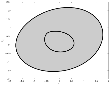
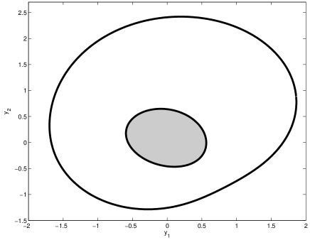
Figure 2: Left: LMI set ${\mathcal{F}}(A)$ (gray area) delimited by the inner oval of quartic $\mathcal{P}$ (black line). Right: numerical range ${\mathcal{W}}(A)$ (gray area) delimited by the outer oval of octic $\mathcal{Q}$ (black line).

For

$$A=\left[\begin{array}[]{cccc}0&2&1+2i&0\\ 0&0&1&0\\ 0&i&i&0\\ 0&-1+i&i&0\end{array}\right]$$

the quartic $\mathcal{P}$ and its dual octic $\mathcal{Q}$ both feature two nested ovals, see Figure 2. The inner oval delimited by $\mathcal{P}$ is rigidly convex, whereas the outer oval delimited by $\mathcal{Q}$ is convex, but not rigidly convex.

4.3 Cross and star

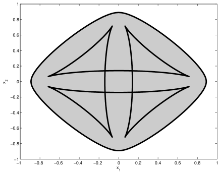
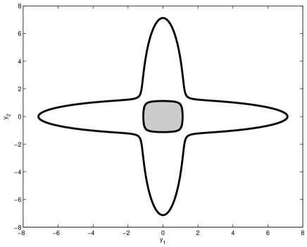
Figure 3: Left: LMI set ${\mathcal{F}}(A)$ (gray area) delimited by the inner oval of quartic $\mathcal{P}$ (black line). Right: numerical range ${\mathcal{W}}(A)$ (gray area) delimited by the outer oval of twelfth-degree $\mathcal{Q}$ (black line).

A computer-generated representation of the numerical range as an enveloppe curve can be found in [7, Figure 1, p. 139] for

$$A=\left[\begin{array}[]{cccc}0&1&0&0\\ 0&0&1&0\\ 0&0&0&1\\ \frac{1}{2}&0&0&0\end{array}\right].$$

We obtain the quartic

$$p(y)=\frac{1}{64}(64y_{0}^{4}-52y_{0}^{2}y_{1}^{2}-52y_{0}^{2}y_{2}^{2}+y_{1}^{4}+34y_{1}^{2}y_{2}^{2}+y_{2}^{4})$$

and the dual twelfth-degree polynomial

$$\begin{array}[]{rcl}q(x)&=&5184x_{0}^{12}-299520x_{0}^{10}x_{1}^{2}-299520x_{0}^{10}x_{2}^{2}+1954576x_{0}^{8}x_{1}^{4}\\ &&+16356256x_{0}^{8}x_{1}^{2}x_{2}^{2}+1954576x_{0}^{8}x_{2}^{4}-5375968x_{0}^{6}x_{1}^{6}-79163552x_{0}^{6}x_{1}^{4}x_{2}^{2}\\ &&-79163552x_{0}^{6}x_{1}^{2}x_{2}^{4}-5375968x_{0}^{6}x_{2}^{6}+7512049x_{0}^{4}x_{1}^{8}+152829956x_{0}^{4}x_{1}^{6}x_{2}^{2}\\ &&-2714586x_{0}^{4}x_{1}^{4}x_{2}^{4}+152829956x_{0}^{4}x_{1}^{2}x_{2}^{6}+7512049x_{0}^{4}x_{2}^{8}-5290740x_{0}^{2}x_{1}^{10}\\ &&-136066372x_{0}^{2}x_{1}^{8}x_{2}^{2}+232523512x_{0}^{2}x_{1}^{6}x_{2}^{4}+232523512x_{0}^{2}x_{1}^{4}x_{2}^{6}-136066372x_{0}^{2}x_{1}^{2}x_{2}^{8}\\ &&-5290740x_{0}^{2}x_{2}^{10}+1498176x_{1}^{12}+46903680x_{1}^{10}x_{2}^{2}-129955904x_{1}^{8}x_{2}^{4}\\ &&+186148096x_{1}^{6}x_{2}^{6}-129955904x_{1}^{4}x_{2}^{8}+46903680x_{1}^{2}x_{2}^{10}+1498176x_{2}^{12}\end{array}$$

whose corresponding curves and convex hulls are represented in Figure 3.

4.4 Decomposition into irreducible factors

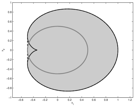
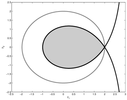
Figure 4: Left: LMI set ${\mathcal{F}}(A)$ (gray area) intersection of cubic (black solid line) and conic (gray line) LMI sets. Right: numerical range ${\mathcal{W}}(A)$ (gray area, black dashed line) convex hull of the union of a quartic curve (black solid line) and conic curve (gray line).

Consider the example of [7, Figure 6, p. 144] with

$$A=\left[\begin{array}[]{ccccccccc}0&0&0&0&1&0&0&0&1\\ 0&0&0&0&0&1&0&0&0\\ 0&0&0&0&0&0&1&0&0\\ 0&0&0&0&0&0&0&1&0\\ 0&0&0&0&0&0&0&0&1\\ 0&0&0&0&0&0&0&0&0\\ 0&0&0&0&0&0&0&0&0\\ 0&0&0&0&0&0&0&0&0\\ 0&0&0&0&0&0&0&0&0\\ \end{array}\right]$$

The determinant of the trivariate pencil factors as follows

$$p(y)=\frac{1}{256}(4y_{0}^{3}-3y_{0}y_{1}^{2}-3y_{0}y_{2}^{2}+y_{1}^{3}+y_{1}y_{2}^{2})(4y_{0}^{2}-y_{1}^{2}-y_{2}^{2})^{3}$$

which means that the LMI set ${\mathcal{F}}(A)$ is the intersection of a cubic and conic LMI.

The dual curve $\mathcal{Q}$ is the union of the quartic

$${\mathcal{Q}}_{\;1}=\{x\>:\>x_{0}^{4}-8x_{0}^{3}x_{1}-18x_{0}^{2}x_{1}^{2}-18x_{0}^{2}x_{2}^{2}+27x_{1}^{4}+54x_{1}^{2}x_{2}^{2}+27x_{2}^{4}=0\},$$

a cardioid dual to the cubic factor of $p(y)$, and the conic

$${\mathcal{Q}}_{\;2}=\{x\>:\>x_{0}^{2}-4x_{1}^{2}-4x_{2}^{2}=0\},$$

a circle dual to the quadratic factor of $p(y)$. The numerical range ${\mathcal{W}}(A)$ is the convex hull of the union of $\mathrm{conv}\>{\mathcal{Q}}_{\;1}$ and $\mathrm{conv}\>{\mathcal{Q}}_{\;2}$, which is here the same as $\mathrm{conv}\>{\mathcal{Q}}_{\;1}$, see Figure 4.

4.5 Polytope

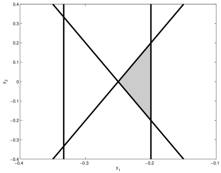
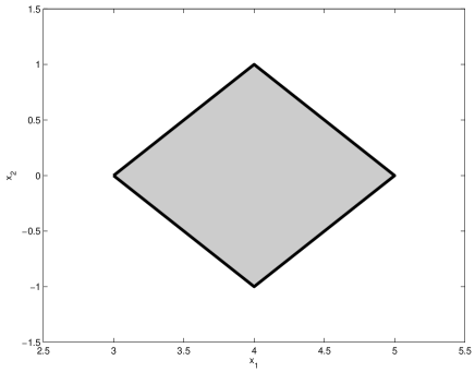
Figure 5: Left: LMI set ${\mathcal{F}}(A)$ (gray area) intersection of four half-planes. Right: numerical range ${\mathcal{W}}(A)$ (gray area) convex hull of four vertices.

Consider the example of [7, Figure 9, p. 147] with

$$A=\left[\begin{array}[]{rrrr}4&0&0&-1\\ -1&4&0&0\\ 0&-1&4&0\\ 0&0&-1&4\end{array}\right].$$

The dual determinant factors into linear terms

$$p(y)=(y_{0}+5y_{1})(y_{0}+3y_{1})(y_{0}+4y_{1}+y_{2})(y_{0}+4y_{1}-y_{2})$$

and this generates a polytopic LMI set ${\mathcal{F}}(A)=\{y\>:\>y_{0}+5y_{1}\geq 0,\>y_{0}+3y_{1}\geq 0,y_{0}+4y_{1}+y_{2}\geq 0,y_{0}+4y_{1}-y_{2}\geq 0\}$, a triangle with vertices $(1,-\frac{1}{4},0)$, $(1,-\frac{1}{5},\frac{1}{5})$ and $(1,-\frac{1}{5},-\frac{1}{5})$. The dual to curve $\mathcal{P}$ is the union of the four points $(1,5,0)$, $(1,3,0)$, $(1,4,1)$ and $(1,4,-1)$ and hence the numerical range ${\mathcal{W}}(A)$ is the polytopic convex hull of these four vertices, see Figure 5.

5 A problem in statistics

We have seen with Example 4.5 that the numerical range can be polytopic, and this is the case in particular when $A$ is a normal matrix (i.e. satisfying $A^{*}A=AA^{*}$), see e.g. [13, Theorem 3] or [7, Theorem 1.4-4].

In this section, we study a problem that boils down to studying rectangular numerical ranges, i.e. polytopes with edges parallel to the main axes. Craig’s theorem is a result from statistics on the stochastic independence of two quadratic forms in variates following a joint normal distribution, see [3] for an historical account. In its simplest form (called the central case) the result can be stated as follows (in the sequel we work in the affine plane $y_{0}=1$):

Theorem 1

Let $A_{1}$ and $A_{2}$ be Hermitian matrices of size $n$. Then $\det(I_{n}+y_{1}A_{1}+y_{2}A_{2})=\det(I_{n}+y_{1}A_{1})\det(I_{n}+y_{2}A_{2})$ if and only if $A_{1}A_{2}=0$.

Proof: If $A_{1}A_{2}=0$ then obviously $\det(I_{n}+y_{1}A_{1})\det(I_{n}+y_{2}A_{2})=\det((I_{n}+y_{1}A_{1})(I_{n}+y_{2}A_{2}))=\det(I_{n}+y_{1}A_{1}+y_{2}A_{2}+y_{1}y_{2}A_{1}A_{2})=\det(I_{n}+y_{1}A_{1}+y_{2}A_{2})$. Let us prove the converse statement.

Let ${a_{1}}_{k}$ and ${a_{2}}_{k}$ respectively denote the eigenvalues of $A_{1}$ and $A_{2}$, for $k=1,\ldots,n$. Then $p(y)=\det(I_{n}+y_{1}A_{1}+y_{2}A_{2})=\det(I_{n}+y_{1}A_{1})\det(I_{n}+y_{2}A_{2})=\prod_{k}(1+y_{1}{a_{1}}_{k})\prod_{k}(1+y_{2}{a_{2}}_{k})$ factors into linear terms, and we can write $p(y)=\prod_{k}(1+y_{1}{a_{1}}_{k}+y_{2}{a_{2}}_{k})$ with ${a_{1}}_{k}{a_{2}}_{k}=0$ for all $k=1,\ldots,n$. Geometrically, this means that the corresponding numerical range ${\mathcal{W}}(A)$ for $A=A_{1}+iA_{2}$ is a rectangle with vertices $(\min_{k}a_{k},\min_{k}b_{k})$, $(\min_{k}a_{k},\max_{k}b_{k})$, $(\max_{k}a_{k},\min_{k}b_{k})$ and $(\max_{k}a_{k},\max_{k}b_{k})$.

Following the terminology of [14], $A_{1}$ and $A_{2}$ satisfy property L since $y_{1}A_{1}+y_{2}A_{2}$ has eigenvalues $y_{1}{a_{1}}_{k}+y_{2}{a_{2}}_{k}$ for $k=1,\ldots,n$. From [14, Theorem 2] it follows that $A_{1}A_{2}=A_{2}A_{1}$, and hence that the two matrices are simultaneously diagonalisable: there exists a unitary matrix $U$ such that $U^{*}A_{1}U=\mathrm{diag}_{k}{a_{1}}_{k}$ and $U^{*}A_{2}U=\mathrm{diag}_{k}{a_{2}}_{k}$. Since ${a_{1}}_{k}{a_{2}}_{k}=0$ for all $k$, we have $\sum_{k}{a_{1}}_{k}{a_{2}}_{k}=U^{*}A_{1}UU^{*}A_{2}U=U^{*}A_{1}A_{2}U=0$ and hence $A_{1}A_{2}=0$. $\Box$

6 Conclusion

The geometry of the numerical range, studied to a large extent by Kippenhahn in [13] – see [18] for an English translation with comments and corrections – is revisited here from the perspective of semidefinite programming duality. It is namely noticed that the numerical range is a semidefinite representable set, an affine projection of the semidefinite cone, whereas its geometric dual is an LMI set, an affine section of the semidefinite cone. The boundaries of both primal and dual sets are components of algebraic plane curves explicitly formulated as locii of determinants of Hermitian pencils.

The notion of numerical range can be generalized in various directions, for example in spaces of dimension greater than two, where it is non-convex in general [4]. Its convex hull is still representable as a projection of the semidefinite cone, and this was used extensively in the scope of robust control to derive computationally tractable but potentially conservative LMI stability conditions for uncertain linear systems, see e.g. [16].

The inverse problem of finding a matrix given its numerical range (as the convex hull of a given algebraic curve) seems to be difficult. In a sense, it is dual to the problem of finding a symmetric (or Hermitian) definite linear determinantal representation of a trivariate form: given $p(y)$ satisfying a real zero (hyperbolicity) condition, find Hermitian matrices $A_{k}$ such that $p(y)=\det(\sum_{k}y_{k}A_{k})$, with $A_{0}$ positive definite. Explicit formulas are described in [9] based on transcendental theta functions and Riemann surface theory, and the case of curves $\{y\>:\>p(y)=0\}$ of genus zero is settled in [10] using Bézoutians. A more direct and computationally viable approach in the positive genus case is still missing, and one may wonder whether the geometry of the dual object, namely the numerical range $\mathrm{conv}\{x\>:\>q(x)=0\}$, could help in this context.

References

• [1] A. Ben-Tal, A. Nemirovski. Lectures on modern convex optimization. SIAM, 2001.
• [2] C. C. Cowen, E. Harel. An effective algorithm for computing the numerical range. Technical report, Department of Mathematics, Purdue University, 1995.
• [3] M. F. Driscoll, W. R. Gundberg Jr. A history of the development of Craig’s theorem. The American Statistician, 40(1):65-70, 1986.
• [4] M. K. H. Fan, A. L. Tits. On the generalized numerical range. Linear and Multilinear Algebra, 21(3):313-320, 1987.
• [5] M. Fiedler. Geometry of the numerical range of matrices. Linear Algebra and its Applications, 37:81-96, 1981.
• [6] I. M. Gelfand, M. M. Kapranov, A. V. Zelevinsky. Discriminants, resultants and multidimensional determinants. BirkhΓ€user, 1994.
• [7] K. E. Gustafsson, D. K. M. Rao. Numerical range: the field of values of linear operators and matrices. Springer, 1997.
• [8] J. Harris. Algebraic geometry: a first course. Springer, 1992.
• [9] J. W. Helton, V. Vinnikov. Linear matrix inequality representation of sets. Communications in Pure and Applied Mathematics, 60(5):654–674, 2007.
• [10] D. Henrion. Detecting rigid convexity of bivariate polynomials. International Symposium on Mathematical Theory of Networks and Systems (MTNS), 2008.
• [11] N. J. Higham. The matrix computation toolbox. Version 1.2, 2002.
• [12] R. A. Horn, C. R. Johnson. Topics in matrix analysis. Cambridge University Press, 1991.
• [13] R. Kippenhahn. Über den Wertevorrat einer Matrix. Mathematische Nachrichten, 6(3-4):193-228, 1951.
• [14] T. S. Motzkin, O. Taussky. Pairs of matrices with property L. Transactions of the American Mathematical Society, 73(1):108-114, 1952.
• [15] F. D. Murnaghan. On the field of values of a square matrix. Proceedings of the National Academy of Sciences of the United States of America, 18(3):246-248, 1932.
• [16] A. Packard, J. Doyle. The complex structured singular value. Automatica, 29(1):71-109, 1993.
• [17] R. J. Walker. Algebraic curves. Princeton University Press, 1950.
• [18] P.F. Zachlin, M.E. Hochstenbach. On the numerical range of a matrix. Linear and Multilinear Algebra, 56(1-2):185-225, 2008. English translation with comments and corrections of [13].