Pulling self-interacting polymers in two-dimensions

Abstract

We investigate a two-dimensional problem of an isolated self-interacting end-grafted polymer, pulled by one end. In the thermodynamic limit, we find that the model has only two different phases, namely a collapsed phase and a stretched phase. We show that the phase diagram obtained by Kumar at al.  [Phys. Rev. Lett. 98, 128101 (2007)] for small systems, where differences between various statistical ensembles play an important role, differ from the phase diagram obtained here in the thermodynamic limit.

I Introduction

The physics of single polymer chains in a poor solvent is still not very well understood. Away from the $\theta$-temperature, we know that a polymer will be in either a collapsed or a swollen state degennes . The mean-square radius of gyration $\langle R^{2}\rangle_{g}$ scales with chain length $N$ as $\langle R^{2}\rangle_{g}\sim const.\times N^{2\nu},$ where $\nu$ is a critical exponent. At low temperatures, when the polymer is in the collapsed state, $\nu=1/d$ while at high temperatures an “extended” or “swollen coil” state exists where $\nu=1,3/4,0.588\ldots,1/2$ for $d=1,2,3,4$ degennes respectively. These values are believed to be exact for $d=1,2$ and, with a logarithmic correction, for $d=4.$ At high temperatures stretching a polymer should produce a state where $\nu=1$ which we shall refer to as the “stretched” state. Although there are many theoretical marenduzzo2003a-a ; rosa2003a-a ; orlandini2004a-a as well as experimental strick2001a-a works on pulling of a collapsed chain, it seems that some issues remain to be fully understood.

Recently Kumar et al. presented results jensen2007 from exact enumeration of force-induced polymer unfolding in two dimension in the context of modeling single molecule experiments. For finite systems, they proposed a phase diagram, which has three phases namely a collapsed phase, an extended phase and a stretched phase (in addition there is a swollen phase which only occurs at $F=0$ above the $\theta$-temperature). They found a transition line between the stretched state and the extended phase. The phase diagram proposed is presented in Fig. 1. The lower phase boundary was obtained in both the constant force and constant temperature ensembles, and indicates a phase-transition line where polymer goes from the collapsed phase to the extended state. However, the upper phase boundary was been only in the constant force ensemble and it was proposed that this represents a transition line where the polymer goes from the stretched state to the extended state.

At this point it is pertinent to mention that very few attempts have been made to perform single molecule experiments in the constant force ensemble. Only recently did Danilowicz et al. danilowicz perform stretching experiments on single stranded DNA in the constant force ensemble. It was observed that at low force, the extension increases with temperature, while at high force the extension decreases with temperature. Kumar and Mishra kumar2008 found that this decrease is an entropic effect and showed that the upper line is not a true phase transition but a crossover effect.

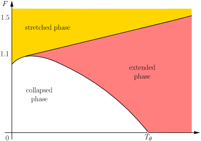
Figure 1: Schematic phase diagram proposed by Kumar et al. jensen2007 .

In this paper we focus our attention on the true nature of the phase-diagram for the model in the thermodynamic limit. We present some further studies of the series data trying to gauge the scaling behavior of the model at different points in the phase-diagram. While somewhat inconclusive our analysis does indicate that the true phase-diagram (for non-zero force) has only two distinct phases for non-zero forces and not three as originally conjectured. The extended phase does not exist for non-zero forces and the upper phase boundary is a finite-size effect only present when the model is studied at fixed force with a variable temperature.

Hence to really delineate the phase diagram we have also performed Monte Carlo simulations using the FlatPERM algorithm prellberg2004 . We investigate several hypothetical phase diagrams. In particular, we consider the possible scenario that the phases seen are two types of stretched phase; one where the polymer is maximally stretched in a rod-like conformation and the other where $\nu=1$ though the polymer is not maximally stretched. Using the simulation results we are able to confidently deduce that there is no evidence of any additional phase or phase transition.

We would like to emphasise that the “phase diagram” obtained by Kumar at al.  jensen2007 for small systems may still be relevant in the context of experiments on bio-polymers. In real systems of finite size differences between various statistical ensembles do play an important role as evidenced not only by this previous study but also by recent experimental work danilowicz . We thus see our discovery of a discrepancy between the finite size “phase diagram” and the true infinite size phase diagram as an important contribution to a better understanding of the types of finite-size effects that may be of importance to the interpretation and understanding of experimental results on small systems.

In section II we define the model. In section III we first briefly review the evidence presented using series analysis to support the conjectured phase-diagram jensen2007 ; jensen2008 and then present further results from a more thorough and extensive analysis of the series data casting doubt on the upper phase boundary of the proposed phase-diagram. In section IV we present the conclusive results of the Monte Carlo simulations which do not support the existence of any additional phase transitions: we carefully consider various possible scenarios. Finally, in section V we summarize our final conclusions.

II Model

We model the polymer chains as interacting self-avoiding walks (ISAWs) on the square lattice as shown in Fig. 2. Interactions are introduced between non-bonded nearest neighbor monomers. In our model one end of the polymer is attached to an impenetrable neutral surface (there are no interactions with this surface) while the polymer is being pulled from the other end with a force acting in the direction perpendicular to the surface. Note that the ISAW does not extend beyond either end-point so the $y$-coordinate $y_{j}$ of the $j$’th monomer is restricted by $0=y_{0}\leq y_{j}\leq y_{N}=h$.

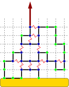
Figure 2: The model of a polymer on the two dimensional square lattice pulled by the last monomer. The arrow indicates the direction of the pulling force. The dark (red) filled circles on lattice sites denote monomers interacting via nearest-neighbor interactions.

We introduce Boltzmann weights $\omega=\exp(-\varepsilon/k_{\rm B}T$) and $u=\exp(F/k_{\rm B}T)$ conjugate to the nearest neighbor interactions and force, respectively, where $\varepsilon$ is the interaction energy, $k_{\rm B}$ is Boltzmann’s constant, $T$ the temperature and $F$ the applied force. In the rest of this study we set $\varepsilon=-1$ and $k_{\rm B}=1$. We study the finite-length partition functions

$$Z_{N}(T,F)=\sum_{\rm all\ walks}\omega^{m}u^{h}=\sum_{m,h}C_{N,m,h}\omega^{m}u^{h},$$ (1)

where $C_{N,m,h}$ is the number of ISAWs of length $N$ having $m$ nearest neighbor contacts and whose end-point is a distance $h$ from the surface.

III Series Analysis

III.1 Fluctuation curves and the conjectured phase diagram

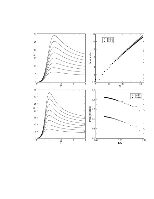
Figure 3: The fluctuations in the number of contacts as a function of temperature for fixed force $F=0.0$ (upper left panel) and $F=0.5$ (lower left panel). Each panel contains curves for ISAWs of length (from bottom to top) $N=20,25,\ldots,55$. In the upper right panel we show a log-log plot of the growth in the peak value of the fluctuation curve with chain length $N$. The lower right panel shows the peak position (critical temperature value) vs $1/N$.

To begin let us recall the type of analysis presented by Kumar et al. jensen2007 ; jensen2008 . At low temperature and force the polymer chain is in the collapsed state and as the temperature is increased (at fixed force) the polymer chain undergoes a phase transition to an extended state. The value of the transition temperature (for a fixed value of the force) can be obtained from the fluctuations in the number of non-bonded nearest neighbor contacts. The fluctuations are defined as $\chi=\langle m^{2}\rangle-\langle m\rangle^{2}$, with the $k$’th moment given by

$$\langle m^{k}\rangle=\frac{\sum_{m,h}\!m^{k}C(N,m,h)\omega^{m}u^{h}}{\sum_{m,h}\!C(N,m,h)\omega^{m}u^{h}}.$$

In the panels of Fig. 3 we show the emergence of peaks in the fluctuation curves with increasing $N$ at fixed force $F=0.0$ and $F=0.5$. In the top right panel we show the growth in the peak value as $N$ is increased. Since this is a log-log plot we see that the peak values grows as a power-law with increasing $N$; this divergence is the hall-mark of a phase transition. In the lower right panel we have plotted the position of the peak (or transition temperature) as a functions of $1/N$. Clearly the transition temperature appears to converge to a finite (non-zero) value but the data exhibits clear curvature which makes an extrapolation to infinite length difficult.

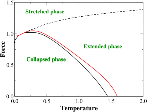
Figure 4: The finite-size ‘phase diagram’ for flexible chains as obtained from the position of the peak in the contact fluctuation curves for $N=55$. The solid black curve and the dashed curve are obtained by fixing the force and varying the temperature.

In Fig. 4, we show the force-temperature ‘phase diagram’ for flexible chains as obtained from the peak positions for the finite chains. However, true phase diagram should be obtained by extrapolating the data to the $N\to\infty$ limit). In Fig. 4 we have shown the transitions as obtained by fixing the force (black curves). One of the most notable feature of the phase-diagram is the re-entrant behavior but this has been studied and explained in previous papers jensen2007 ; jensen2008 . The other notable feature is that in the fixed force case we see an apparent new transition line from the extended state to the fully stretched state which is solely induced by the applied force (the dashed line in Fig. 4).

III.2 Further series analysis results

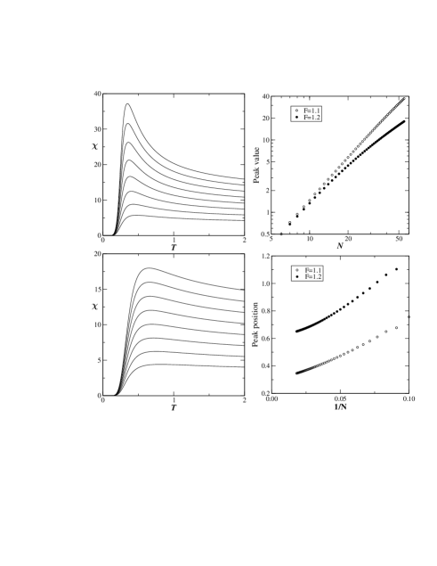
Figure 5: Same as in Fig. 3 but for fixed force $F=1.1$ (upper left panel) and $F=1.2$ (lower left panel).

In Fig. 5 we have plotted the fluctuation curves for force $F=1.1$ and $F=1.2$. The curves for $F=1.1$ (including the plot of the peak height) looks very similar to the plots (see Fig. 6) for low values of the force. For force $F=1.2$ the peak is not very pronounced and we are hesitant to even call it a peak. Also when we look at the peak height vs. $N$ it appears that the curve has two different behaviors for small and large $N$, respectively. This could be a sign of a cross-over behavior.

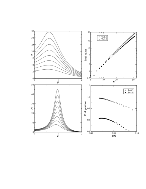
Figure 6: The fluctuations in the number of contacts as a function of force for fixed temperature $T=1.0$ (upper left panel) and $T=0.5$ (lower left panel). Each panel contains curves for ISAWs of length (from bottom to top) $N=20,25,\ldots,55$. In the upper right panel we show a log-log plot of the growth in the peak value of the fluctuation curve with chain length $N$. The lower right panel shows the peak position (critical force value) vs $1/N$.

One can also study the same transition phenomenon by fixing the temperature and varying the force. In the panels of Fig. 6 we show the emergence of peaks in the fluctuation curves with increasing $N$ at fixed temperature $T=1.0$ and $T=0.5$. Again we observe the power-law divergence of the peak-value. The only other note-worthy feature is that in the plots of the peak position (critical force value) we observe not only strong curvature but we actually see a turning point in the curves as $N$ is increased. This feature would make it impossible (given the currently available chain lengths) to extrapolate this data. However, we do not observe the upper transition line in this study where we have fixed the temperature and varied the force. Indeed this is clear from Fig. 6 where at fixed $T=0.5$ and $1.0$ we see only a single peak (giving us points on the red curve in the ‘phase diagram’ Fig. 4).

In Fig. 6 the value of the force extends up to $F=2.0$ and the upper transition (dashed line in the phase diagram) should appear (if present) as a second peak in the fluctuation curves of Fig. 6. The absence of any evidence of a second peak is what leads us conclude that we do not see this second transition in the fixed $T$ varying $F$ study.

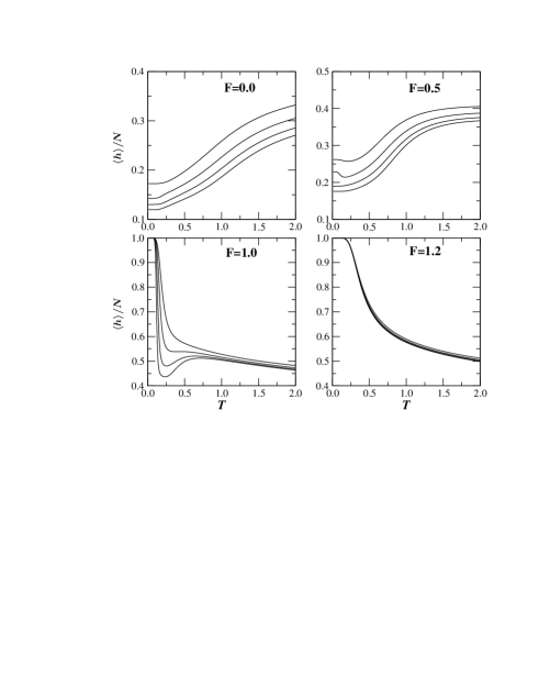
Figure 7: The average extension per monomer $\langle h\rangle/N$ as a function of temperature $T$ for different values of the force. Each panel contain four curves for, from top to bottom, $N=25$, 35, 45, and 55.

In Fig. 7 we have plotted the average extension per monomer $\langle h\rangle/N$ as a function of temperature. In the case of a fixed force $F=1.2$ (lower right panel) we note that curves for different values of $N$ more or less coincide showing that the average extension scales like $N$ for all temperatures. We contend that this observed behavior shows that the upper boundary is a crossover effect supporting the finding reported recently by Kumar and Mishra kumar2008 .

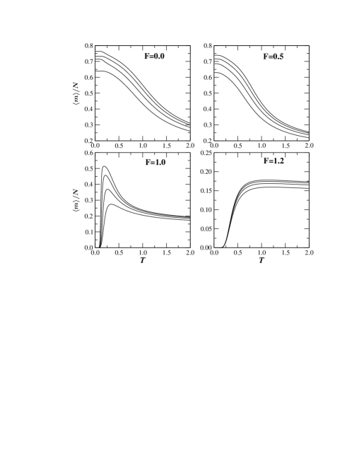
Figure 8: The average number of contacts per monomer $\langle m\rangle/N$ as a function of temperature $T$ for different values of the force. Each panel contain four curves for, from bottom to top, $N=25$, $35$, $45$, and $55$.

In Fig. 8 we have plotted the average number of contacts per monomer $\langle m\rangle/N$ as a function of temperature. In the case of a fixed force $F=1.2$ (lower right panel) we note that curves for different values of $N$ more of less coincide showing that the average extension scales like $N$ for all temperatures.

IV Simulation results

Our more detailed analysis of the series indicates that the upper phase boundary is not a real phase transition.. To further investigate the model we have turned to Monte Carlo simulations that allow analysis of longer polymer chains. We have chosen to use the FlatPERM algorithm prellberg2004 to simulate the model. One advantage of FlatPERM, as a “flat histogram” technique, is the ability to sample the density of states uniformly with respect to a chosen parametrisation, so that the whole parameter range is accessible from one simulation. This allows us to “see” the phase diagram from one set of results. The cost of this however is that the chain lengths that can be simulated accurately are still fairly modest. We have performed “whole phase space” simulations up to length $N=128$. On the other hand by restricting interest to sub-manifolds of the parameter space longer chains can be analyzed. We have performed simulations along various lines and at points in the phase diagram using walks up to length $N=1024$. The schematic phase diagram conjectured by Kumar et al. jensen2007 ; jensen2008 is shown in Fig. 9 along with special lines considered in our simulations.

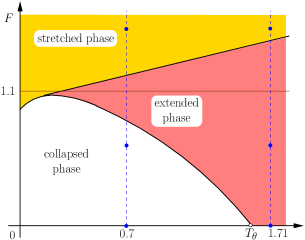
Figure 9: Schematic phase diagram conjectured by Kumar et al. jensen2007 ; jensen2008 . The conjectured phase diagram has three different phases: ‘collapsed’, ‘extended’ and ‘stretched’. We have performed simulations of the whole phase space up to length $N_{max}=128$. The dashed lines at fixed temperatures $T=0.7$ and $T=1.71$ display lines along which simulations were performed for walk lengths up to $N_{max}=1024$. The six points displayed are those at which we have focused our attention.

To demonstrate what is estimated in a FlatPERM simulation consider for a moment a general polymer model with microscopic energies $-\varepsilon_{1}$, $-\varepsilon_{2}$, etc associated with configurational parameters $m_{1}$, $m_{2}$ respectively. Let the density of states be $C_{N,m_{1},m_{2},\dots}$. Then the partition function is given by

$$Z_{N}(\beta_{1},\beta_{2},\dots)=\sum_{m_{1},m_{2},\dots}C_{N,m_{1},m_{2},\dots}\;e^{\beta_{1}m_{1}+\beta_{2}m_{2}+\dots},$$ (2)

where $\beta_{1}=\beta\varepsilon_{1}$, $\beta_{2}=\beta\varepsilon_{2}$ etc, and $\beta=\frac{1}{k_{B}T}$, with $k_{B}$ Boltzmann’s constant. FlatPERM can estimate $C_{N,m_{1},m_{2},\dots}$ or any sum of the $C_{N,m_{1},m_{2},\dots}$ over any number of the $m_{j}$ for a range of lengths $N\leq N_{max}$. If one finds $C_{N,m_{1},m_{2},\dots}$ then one can estimate average quantities over this distribution for any values of $\beta_{1},\beta_{2},\dots$. In our model we have $m_{1}=m$ and $m_{2}=h$ with $\beta_{1}=1/T$ and $\beta_{2}=F/T$. We have performed simulations over the complete space of the variables $m$ and $h$ for $N\leq N_{max}=128$. In this way we have estimated the density of states $C_{N,m,h}$. We performed $10$ different runs with this parametrisation for lengths up to $N_{max}=128$. We have estimated the average number of contacts per monomer $\langle m\rangle/N$ and the average extension per step $\langle h\rangle/N$ and their fluctuations $\sigma^{2}(m)/N$ and $\sigma^{2}(h)/N$.

Previous work (see bennett-wood1998 and references therein) has estimated the $\theta$-point to be around $T=1/0.663=1.51$. With this in mind we have also performed one-parameter simulations with $T$ fixed at $T=0.7$ and at $T=1.71$. The temperatures chosen were to ensure that one temperature was below and one was above the $\theta$-temperature as shown in Fig. 9. We also studied the temperature $T=2.0$ with $F=0$ as a high temperature point.

In order to delineate the possible phases we considered the points $F=0.0,0.5,1.5$ for $T=0.7$ and $1.71$ and also the point $T=2.0$, $F=0$. In particular, we analyzed the scaling of the end-to-end distance $R^{2}_{N}$ which gives an estimate of the exponent $\nu$. Let us start with $F=0$. For $T=2.0$ we expect that the polymer is in the extended phase with $2\nu=1.5$ and in Fig. 10 we find precisely that. For $T=0.7$ we expect the polymer to be in the collapsed phase with $2\nu=1.0$ and once again our data in Fig. 11 confirms this expectation. Now let us move to $F=0.5$. For the low temperature $T=0.7$ the series data places this point in the collapsed phase and the data in Fig. 11 bears this out.

However, for the point $F=0.5$ with $T=1.71$ the conjectured phase diagram of Kumar et al. jensen2007 predicts this point to be in the extended phase with $2\nu=1.5$ while we find that $2\nu=2.00(2)$, so this point is in the stretched phase. For $F=1.5$ and for $T=0.7$ and $T=1.1$ the conjectured phase diagram predicts a stretched phase with a value of $2\nu=2$ and we confirm this as seen from Fig. 12.

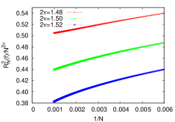
Figure 10: End-to-end distance divided by $N^{2\nu}$ against $1/N$ for point, $(T,F)=(2.0,0.0)$. We see $2\nu=1.5(2)$. This point is in the extended phase.

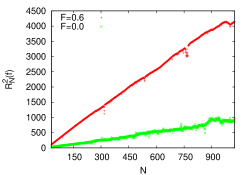
Figure 11: End-to-end distance divided by $N^{2\nu}$ against $N$ for two points, $(T,F)=(0.7,0.0)$ and $(T,F)=(0.7,0.6)$ for lengths up to $N=1024$. A clear linear dependence is seen implying $2\nu\approx 1$. These points are in the collapsed phase and this exponent result is consistent with this assumption.

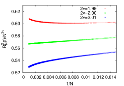
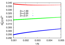
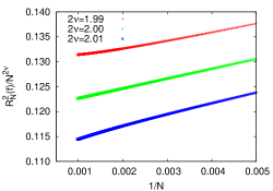
Figure 12: End-to-end distance divided by $N^{2\nu}$ against $1/N$ for three points, $(T,F)=(0.7,1.5)$, $(1.71,1.5)$, and $(1.71,0.6)$. for length up to $N=1024$. We conclude, that all these points belong to a stretched phase of same type, where $\nu=1.0$.

It is clear that the assumption of an extended phase for $F>0$ is incorrect. However, while mistakenly named perhaps three phases still exist for $F>0$. Considering the series results the other possibility is that the extended phase is indeed stretched with $\nu=1$ for $F>0$ and that the “stretched” phase described in Kumar et al. jensen2007 ; jensen2008 is really a “fully stretched” phase where in addition to $\nu=1$ the average height per step converges to unity:

$$\lim_{N\rightarrow\infty}\frac{\langle h\rangle}{N}=1.$$ (3)

That is, the configurations of the polymer are essentially rod-like (with sub-dominant fluctuations). For such rod-like configurations one would also expect in this phase that

$$\lim_{N\rightarrow\infty}\frac{\langle m\rangle}{N}=0.$$ (4)

A revised conjectured phase diagram is drawn in Fig. 13, along with our lines of longer length simulations and the points at which we have focused our analysis. The series data in Fig. 7 and 8 for the low temperature regions when $F=1.2$ display behavior resembling that delineated above for a possible “fully stretched” phase.

Figure 13: Here is a second possible phase digram assuming there are two phases for non-zero forces, both with $\nu=1$. Instead of extended and stretched we have “fully stretched” and stretched. In such a hypothesized “fully stretched” phase the polymer is effectively in a rod-like conformation where the average height is approximately equal to the length of the polymer.

To search for possible phase transitions we have estimated the fluctuations in the number of contacts and fluctuations in the height. For fixed force $F=1.4$ the plot of the fluctuation against temperature in Fig. 14 shows no sign of a growing singularity for lengths up to $N=128$ as seen in the series data for shorter lengths and smaller forces.

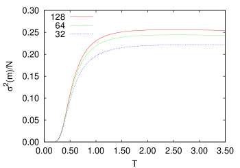
Figure 14: The fluctuations in the number of contacts $m$ for $F=1.4$ fixed plotted against temperature $T$. There is no sign of any growing singularities which would indicate a phase transition in the thermodynamic limit.

Now we consider the fixed temperature lines at $T=1.71$ and $T=0.7$. For $T=1.71$ the only sign of a singularity appears near $F=0$ (see Fig. 15), that is the expected sign of the transition from the extended phase at $F=0$ to the stretched phase at $F>0$.

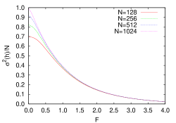
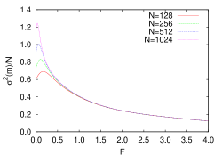
Figure 15: Plots of the fluctuations against force $F$ for the high temperature $T=1.71$.

For $T=0.7$ again there is only a sign of a single phase transition in either the fluctuations of $m$ and $h$ (see Fig. 15).

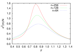
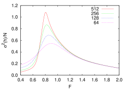
Figure 16: Plots of the fluctuations against force $F$ for the low temperature $T=0.7$

Now the question may be asked about the nature of the peaks in the fluctuations seen at low temperatures at forces just above $F=1$. In Fig. 17 we plot the maximum in the fluctuations at fixed force for various values between $F=1.1$ and $F=1.2$. We note that while these peaks do exist they are not indicative of any divergences. Of course there may still be a weak phase transition. We now turn our attention to any possible difference in the conformations of the polymer in the regions labeled “stretched” and “fully stretched”.

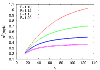
Figure 17: The maximum of the fluctuations in the number of contacts $m$ for lengths from $N=32$ up to $N=128$ for four different forces in the region where the original series data analysis detected a phase transition.

To test the hypothesis on which the revised conjectured phase diagram (Fig. 13) rests we consider the scaling of the average height of the last monomer. In Fig. 18 we plot the height of the last monomer at six different points for temperatures $T=0.7$ and $T=1.71$. We observe that at the three points $(T,F)=(0.7,1.5),(1.71,1.5)\mbox{ and }(1.71,0.6)$ the average height converges to a non-zero, and importantly, non-unity value. Also, at the remaining three points, while there are clear non-linear corrections to scaling, the average converges to zero. In other words no indication of a fully stretched phase can be found.

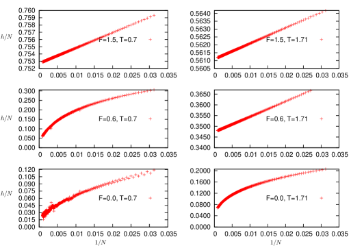
Figure 18: The height of the last monomer at six different points depicted in Fig. 9. We see that in all cases the height of the last monomers does not converge to $1$, which we would expect for a fully stretched phase for figures at $F=1.5,T=0.7$ and $T=1.71$ and for $F=0.6,T=1.71$.

A further test of the hypotheses leading to the revised conjectured phase diagram (Fig. 13) can be carried out. We assumed that for very low temperatures and large finite forces the average number of contacts per step goes to zero. To test this we have plotted $\left<m\right>$ against $1/N$ for $F=1.2$ with $T=0.1$ in Fig. 19. While small (of the order of $10^{-6}$) this quantity is strictly increasing with length and clearly converges to a (small) non-zero value.

Figure 19: The behavior of the average number of bulk contacts $\left<m\right>$ for length $N=32$ up to $N=128$ for the point $T=0.1$, $F=1.2$ as a function of $1/N$. We observe an increase in the average number of contacts $\left<m\right>$ with $N$ even for very low temperatures.

We therefore conclude that the upper phase boundary proposed in jensen2007 ; jensen2008 does not exist in the thermodynamic limit and the revised phase diagram in the thermodynamic limit is shown in Fig. 20.

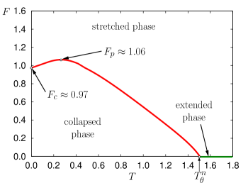
Figure 20: The finite-size phase diagram of a self-interacting self-avoiding walk under tension in two dimensions for length $N=128$. We have estimated the position of the maximum force $F_{p}$, and the force $F_{c}$ for $T=0.0$. The $T^{N}_{\theta}\approx 1.47$. One would expect that $F_{c}=1.0$ in the thermodynamic limit.

Finally we attempt to measure the exponents associated with the collapse to stretched phase transition. This seems to be a second order phase transition with divergent specific heat. In Fig. 21 we plot the logarithm of the fluctuations in the number of contacts per monomer $m/N$ against $\log(N)$. The data in this plot is obtained at $T=0.074$ and at the force $F$ for which the fluctuations are maximal. From the date we obtain estimates of the specific heat exponent $\alpha=0.62(10)$ and the crossover exponent $\phi=0.72(6)$. The divergence of the finite size specific heat is expected to be controlled by the exponent $\alpha\phi$ and the two exponents are expected to by related via the scaling relation $2-\alpha=1/\phi$.

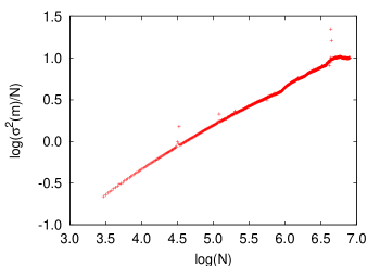
Figure 21: The logarithm of the fluctuation in the number of contacts per monomer $m/N$ against $\log(N)$ at $T=0.074$ for the force $F$ at which the fluctuations are maximal. From this curve we can estimate the exponents $\alpha=0.62(10)$ and $\phi=0.72(6)$, which we note are not those of the two-dimensional $\theta$-transition.

V Summary

In summary we have shown that for a model of self-interacting polymers pulled away from a surface in two dimension there are only two different phases for non-zero forces in the thermodynamic (infinite length) limit. We therefore conjecture a generic phase diagram as in Fig. 22.

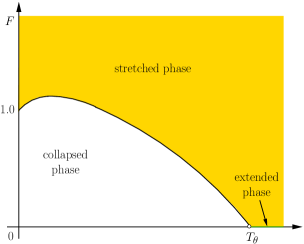
Figure 22: The final conjectured phase diagram for a two-dimensional self-interacting polymer under a stretching force arising from our analysis in this work.

One of the phases is the collapsed phase, which is driven by the temperature at small forces. The other is a single stretched phase which occurs whenever the force is applied for temperatures higher than the $\theta$-temperature, and for large enough forces for small temperatures. Importantly, the polymer is only in a fully stretched state at zero temperature for forces $F\geq F_{c}=1$ or when the applied force is infinite.

References

- (1) P. G. de Gennes Scaling Concepts in Polymer Physics (Cornell University Press: Ithaca, 1979).
- (2) D. Marenduzzo, A. Maritan, A. Rosa, and F. Seno, Phys. Rev. Lett. 90, 088301 (2003).
- (3) A. Rosa, D. Marenduzzo, A. Maritan, and F. Seno, Phys. Rev. E. 67, 041802 (2003).
- (4) E. Orlandini, M. Tesi, and S. Whittington, J. Phys. A: Math. Gen. 37, 1535 (2004).
- (5) T. Strick, J.-F. Allemand, V. Croquette, and D. Bensimon, Phys. Today 54, 46 (2001).
- (6) S. Kumar, I. Jensen, J. L. Jacobsen and A. J. Guttmann, Phys. Rev. Lett. 98, 128101 (2007).
- (7) C. Danilowicz, C. H. Lee, V. W. Coljee, and M. Prentiss, Phys. Rev. E, 75 030902(R) (2007).
- (8) S. Kumar and G. Mishra, Phys. Rev. E, 78 011907 (2008).
- (9) T. Prellberg and J. Krawczyk, Phys. Rev. Lett. 92, 120602 (2004).
- (10) A. J. Guttmann, J. L. Jacobsen, I. Jensen and S. Kumar, J. Math. Chem. (to appear). Preprint: arXiv:0711.3482
- (11) D. Bennett-Wood, I.G. Enting, D. S. Gaunt, A. J. Guttmann, J. L. Leask, A. L. Owczarek and S. G. Whittington, J. Phys. A: Math. Gen. 31, 4725 (1998).